Inversion of marine heat flow measurements by expansion of the temperature decay function

Marine heat flow data, obtained with a Lister-type probe, consists of two temperature decay curves, frictional and heat pulse decay. Both follow the same physical model of a cooling cylinder. The mathematical model describing the decays is nonlinear as to the thermal sediment parameters thus a direct inversion is not possible. To overcome this difficulty, the model equations are expanded using a first order Taylor series. The linearised model equations are used in an iterative scheme to invert the temperature decay for undisturbed temperature and thermal conductivity of the sediment. The inversion scheme is tested first for its theoretical limitations using synthetic data. Inversion of heat flow measurements obtained during a cruise of R/V SONNE in 1996 and needle probe measurements in material of known thermal conductivity show that the algorithm is robust and gives reliable results. The program can be obtained from the authors.

Introduction

The growing interest in global energy and geochemical fluxes in the oceans and the availability of multi-penetration heat flow probes have has led to increased attention in marine geothermal studies, which are mainly focused on the sediment covered areas of ridges and ridge flanks. Studies of accretionary wedges that incorporate heat flow investigations also reflect the need for additional constraints to model and understand the dewatering process of accreted sediments. This increased interest in marine heat flow data has helped to improve the existing measurement technique in two ways: The violin bow type heat probe instrument, as described in Hyndman et al., (1979), has evolved over two decades of intensive use to a mature, mechanically robust instrument which now can be used in a routine way. Rapid electronic development led to an increased temperature resolution of 1 mK and allowed a larger number of sensors to be mounted on one string due to increased storage capacity. Both developments now permit multi-penetration deployments (measurements in a pogo-style fashion) of up to 24 hours per station. Advances in marine navigation now permit very detailed studies of regional processes. Worldwide coverage of the Global Positioning System (GPS) and Differential GPS help enormously in station keeping during a measurement. High accuracy in positioning of the probe is achieved by using Long- or Short-Baseline navigation (Jones,, 1999).

Figure 1: Cross section of the sensor tube, housing the temperature sensors (thermistors) and the heating wires for in situ thermal conductivity measurements (see also Table 1).

Part	Layer	$k$	${(\rho c)_{c}}$	Material
		$\left[\frac{\mbox{ W}}{\mbox{m K}}\right]$	$\left[10^{6}\frac{\mbox{ J}}{\mbox{ K m}^{3}}\right]$
Sensor string	1	0.2	2.14	copper, oil, glass
Heating wire	2	13.2	3.50	Ni-Chrome
Oil filling	3	0.2	1.60	oil, plastic
steel tube	4	37.5	3.9	steel

Table 1: Thermal parameters of the sensor tube of figure 1 (after Nagihara & Lister, (1993)).

Figure 1 shows a simplified cross section of a sensor string used by the Heat Flow Group of the University of Bremen (Germany) and the Pacific Geoscience Centre (Sidney, B.C., Canada). The sensors for temperature measurements in the sediment are housed in a hydraulic steel tube with an outer diameter of 8 mm and an internal diameter of 5 mm. Thermal parameters are shown in Table 1 (after Nagihara & Lister, (1993)). The sensor string itself contains heating wires for in situ thermal conductivity measurements and wires leading to the thermistors for temperature measurements. The tube is oil-filled to improve the thermal contact between the temperature sensors and the tube.

In order to illustrate the steps involved to process a heat flow measurement, Fig. 2 shows a typical data set. Measurements of undisturbed sediment temperature and conductivity follow the pulsed needle probe method (Lister,, 1970). When the sensor string penetrates the sediment the friction between sensor tube and sediment creates heat resulting in a temperature rise. The following temperature decay is recorded at 10 s sample rate for a preset time span (7 minutes), after which a calibrated heat pulse of 20 s length is fired. The heat pulse decay is monitored for at least 7 minutes until the probe is pulled out of the sediment and the ship moves to the next measurement position with the probe about 200–300 m above the seafloor (pogo-style measurements).

The processing of the raw measurements requires three steps: (1) determine undisturbed sediment temperatures from frictional decay (2) correct heat pulse decay for the remaining effect of the frictional decay and (3) calculate thermal conductivities from heat pulse decay. The basic design of the processing of heat flow measurements is outlined in Hyndman et al., (1979) which was basically a manual procedure based on the work of Lister, (1970) and Lister, (1979).

The increasing number of measurements per cruise in the past decade required a processing scheme which could easily be implemented on a personal computer for automated processing of a large number of measurements. Villinger & Davis, (1987) published a pragmatic scheme (called HFRED), that minimises the misfit between measured and model data in a least-squares sense by varying the effective origin time of penetration. Tests on numerically modelled data (synthetic measurement) with known parameters showed that HFRED produced reliable and accurate results. However, the scheme has two major deficiencies:

1. The thermal diffusivity used for the sediment is computed from thermal conductivity according to a relationship proposed by Hyndman et al., (1979). This relationship has never been validated by experimental data and will certainly vary with sediment type.

2. The algorithm implemented in HFRED does not allow analysis of errors of the calculated undisturbed sediment temperatures and in-situ thermal conductivities in a rigorous way; errors calculated by HFRED are always unrealistically low, compared to error estimates of about 5% from other studies (Hyndman et al.,, 1979; Lister,, 1970).

To overcome these deficiencies and to incorporate platform independent plotting routines, a mathematically sound inversion scheme of observed temperature decays was implemented using Matlab^®, a widely used software package for numerical analysis. This allows creation of very compact code for the inversion, on-screen graphics and platform-independent plots. In addition, automated processing or reprocessing of a large number of individual measurements is possible. The inversion of the integral describing the decay of a temperature pulse (see equation 1) allows use of the same algorithm for the calculation of undisturbed sediment temperatures (using the frictional decay) and thermal conductivity of the sediment (using the heat-pulse decay). Inversion theory allows calculation of realistic errors in a well-defined and mathematically rigorous way based on the sample rate and temperature resolution used. Contrary to HFRED, the thermal conductivity and diffusivity are treated as independent parameters, which may allow improvement of the relationship of Hyndman et al., (1979).

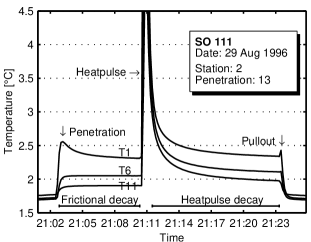
Figure 2: Example of a heat flow measurement. Only three out of 11 sensors are shown.

In the following we propose an inversion scheme, coined T₂C (Temperature to conductivity), that was used to process the heat flow measurements made on the German RV SONNE on the eastern flank of Juan de Fuca during cruise SO111 in the summer of 1996 (Villinger & Fahrtteilnehmer,, 1996). In some concluding remarks we summarise our experience up to now with the new reduction scheme.

1 Theoretical background and inversion scheme

The theoretical background for the analysis of heat flow measurements described in the Introduction is discussed in Bullard, (1954), Lister, (1979), Hyndman et al., (1979), and Villinger & Davis, (1987). The following simplified model for the sensor string is used: A cylinder of radius $a$ and infinite extent in the $z$-direction is situated in a homogenous infinite material. Whereas the material surrounding the cylinder has a finite thermal conductivity $k$ and thermal diffusivity $\kappa$, the cylinder itself is of infinite conductivity and diffusivity, with the constraint that ${(\rho c)_{c}}$, the product of specific heat $c$ and density $\rho$ of the cylinder, remains finite. At time $t=0$, the cylinder is at temperature $T_{0}$ and the ambient space at $T_{a}$. The temperature at the centre $r=0$ of the cylinder can then be described by the thermal decay curve of the cylinder:

$$T(\tau)=(T_{0}-T_{a})\cdot F(\alpha,\tau)+T_{a}$$ (1)

with $F(\alpha,\tau)$ following Bullard, (1954) and Carslaw & Jaeger, (1959):

$$F(\alpha,\tau) = \frac{4\alpha}{\pi^{2}}\int\limits_{0}^{\infty}\frac{e^{-\tau u^{2}}}{u\phi(u,\alpha)}\;du$$ (2)

$$\phi(u,\alpha) = (uJ_{0}(u)-\alpha J_{1}(u))^{2}$$ (3)

$$+(uY_{0}(u)-\alpha Y_{1}(u))^{2}$$

Here $\alpha=2(\rho c)_{s}/(\rho c)_{c}$ is the ratio of the heat capacities per volume of the sediment and the cylinder, and $\tau=\frac{\kappa}{a^{2}}t$ is the dimensionless time. $J_{0}$, $J_{1}$, $Y_{0}$ and $Y_{1}$ are zero and first order Bessel and Neumann functions, respectively and $u$ is the integration variable. The temperature rise $T_{0}-T_{a}$ at time $t=0$ can be expressed by

$$T_{0}-T_{a}=\frac{Q}{\pi a^{2}(\rho c)_{c}}$$ (4)

with $Q$ being the heat per unit length contained in the cylinder. Equation 1 has an asymptotic solution that approximates $F(\alpha,\tau)$ with 1% accuracy for $\tau>10$ (Hyndman et al.,, 1979):

$$T(t)=\frac{Q}{4\pi kt}+T_{a}$$ (5)

It is important to recall the limitations of this model by comparing it with the sensor tube housing the temperature sensors:

1. The sensor tube is non-ideal, i.e. it has a finite conductivity and an internal structure.

2. The duration of the heating pulse is finite, usually in the order of 10–20s.

3. Axial heat flow will be inevitable but certainly small.

4. A thin water-layer between the sediment and the sensor tube may act as insulation to delay the achievement of thermal equilibrium.

Measurements early in the temperature records will be inherently affected by deviations from the model. Therefore, these records have to be excluded from analysis. However, temperatures within the analysed time range still show slight deviations from the ideal behaviour. This deviation can be best modelled by introducing a new parameter, the time shift $t_{s}$. The measured time origin is always the onset of the penetration or heat-pulse. Introduction of the parameter $t_{s}$ approximates the heating of finite length by an instantaneous temperature rise, shifted relative to the onset of the heating. Although mathematically not rigorously proven, this concept is reasonable from a physical point of view and has been shown to provide reliable results (Hyndman et al.,, 1979; Villinger & Davis,, 1987). The justification for using $t_{s}$ will be investigated more thoroughly in section 4 using a numerical model.

The goal of the processing scheme is to invert equation 1. To achieve this, the actual physical parameters have to be restored in equations 2 and 3. This yields

$$T = \frac{8kQ}{\pi^{3}a^{2}\kappa(\rho c)_{c}^{2}}\int\limits_{0}^{\infty}\frac{\displaystyle e^{-u^{2}\frac{\kappa}{a^{2}}(t-t_{s})}}{u\phi(u)}\;du+T_{a}$$ (6)

$$\phi(u) = \left(uJ_{0}(u)-\frac{2k}{\kappa(\rho c)_{c}}J_{1}(u)\right)^{2}$$ (7)

$$+\left(uY_{0}(u)-\frac{2k}{\kappa(\rho c)_{c}}Y_{1}(u)\right)^{2}$$

The equation assumes that the initial temperature $T_{0}$ at $t=0$ is reached by introducing an amount of heat $Q$ either due to frictional heating during penetration or a calibrated heat pulse.

According to equation (6) the temperature decay is a function of six parameters and time:

$$T=T({\bf m},t)\quad\mbox{with}\quad{\bf m}=[k,\kappa,{T_{a}},Q,{(\rho c)_{c}},t_{s}]$$ (8)

The inversion will be demonstrated for the general case of all six parameters being unknown. In practical application of the technique, the number of parameters needs to be reduced. This will be discussed in section 2.

The decay function is nonlinear and cannot be inverted directly. One approach to solve this problem is to expand $T({\bf m},t)$ in terms of a first order Taylor series (Menke,, 1989; Kristiansen,, 1982). The temperature will be expanded around the “true” set of parameters ${\bf r}$, using an estimated set of parameters ${\bf e}$:

$$T({\bf r},t)=T({\bf e},t)+\sum\limits_{i=1}^{6}\left.\frac{\partial T}{\partial m_{i}}\right|_{m_{i}=e_{i}}\underbrace{(r_{i}-e_{i})}_{:=\Delta_{i}}$$ (9)

This equation is linear in the difference vector ${\bf\Delta}$ and can be inverted for this parameter vector. The left side of the equation represents the data and the right side the model. Because the equation is only of first order and hence not exact, a recursive scheme will be used for the calculation of the true parameters whereby the result of the $l$-th iteration is used as an estimate ${\bf e}$ for the $(l+1)$-th iteration.

$${\bf e}^{(l+1)}={\bf e}^{(l)}+{\bf\Delta}^{(l)}$$ (10)

In general ${\bf e}^{(l+1)}$ will be closer to the true parameter set than ${\bf e}^{(l)}$. Because the parameters are of different orders of magnitude, the difference vector ${\bf\Delta}$ has to be normalised so that only relative weights appear in the model kernel (Kristiansen,, 1982).

$$\Delta^{\prime}_{i}=\frac{\Delta_{i}}{e_{i}}\quad i=1,\ldots,6$$ (11)

Applying this method to all data points for times $t_{j}\,(j=1,\ldots,N)$ yields a system of $N$ linear equations. These can be written in matrix notation:

$${\bf G}{\bf\Delta}^{\prime} = {\bf d}$$ (12)

$$G_{j,i} = e_{i}\left.\frac{\partial T({\bf m},t_{j})}{\partial m_{i}}\right|_{\bf m=e}$$ (13)

$$d_{j} = T({\bf r},t_{j})-T({\bf e},t_{j})$$ (14)

${\bf G}$ is the model matrix or kernel, it contains no actual data, only the assumptions of the model. ${\bf\Delta}$ is the model parameter vector and ${\bf d}$ is the data vector.

The solution of the problem requires the inversion of the matrix equation 12 in order to obtain ${\bf\Delta}$. We use singular value decomposition (SVD) closely following Menke, (1989). The decomposition of the model matrix produces three matrices ${\bf G}={\bf U}\cdot{\bf S}\cdot{\bf T^{T}}$ with the solution to the inverse problem:

$${\bf\Delta_{n}}={\bf VS^{-1}U^{T}d}$$ (15)

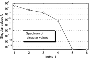
Figure 3: Spectrum of the SVD for a representative set of parameters. For $i>4$, magnitudes are in the range of floating point accuracy of the implementation.

Once conductivity- and temperature-depth profiles are calculated from the decay curves, heat flow values are computed using a method proposed by Bullard, (1939). Starting from the heat diffusion equation for the horizontally layered case,

$$q=\frac{\partial}{\partial z}\left(k(z)T(z)\right)$$ (16)

an integration over depth $z$ yields:

$$T(z)-T_{0}=q\underbrace{\int\limits_{0}^{z}\frac{dz^{\prime}}{k(z^{\prime})}}_{=w}$$ (17)

The integral is called the thermal resistance $w$ and is calculated from the conductivity-depth profile. A linear regression of the temperature profile versus the thermal resistance gives the heat flow density as the slope of

$$T(z)=q\cdot w+T_{0}$$ (18)

2 Processing sequence

In the last section a general inversion scheme was proposed which is capable of inverting frictional and heat pulse decays. It is important that all parameters to be determined are independent of each other. A measure of the linear dependence is the magnitude of the diagonal values $\lambda_{i}$ of the singular matrix ${\bf S}$. A plot of these values is called the spectrum of the singular value decomposition and is shown for a typical temperature decay in figure 3. The accuracy of floating point figures given by Matlab^® is about $10^{-16}$. The spectrum drops to this level after the fourth singular value, suggesting that only four independent parameters can be determined in the problem. However, the accuracy and stability of the inversion is largely influenced by the smallest included singular value and error bounds are proportional to the inverse of the square of this value (Menke,, 1989). Therefore, although it is possible to use four independent parameters, in practice only three parameters were determined to improve the results. A thorough analysis revealed that the singular value $\lambda_{4}$ is mostly influenced by $(\rho c)_{c}$. This observation is a result of the heat capacity being a probe parameter that is only poorly resolved by the model. Therefore a fixed value of 3.38 $\cdot 10^{6}\mbox{ J}/(\mbox{K m}^{3})$ was used, based on the material and geometry of the sensor string (Nagihara & Lister,, 1993). The possibility of a systematic error resulting from a false assumption for the heat capacity will be discussed later.

The restriction to three parameters for one inversion run leads to a certain sequence of processing steps for a single penetration (Villinger & Davis,, 1987):

1. Frictional decay: $Q,T_{a},t_{s}$ are calculated. $k,\kappa,(\rho c)_{c}$ are held fixed, using estimated values for $k$ and $\kappa$.

2. Heat pulse decay: The residual of the frictional decay is subtracted from the heat pulse decay thus reducing the ambient temperature $T_{a}$ to a known value of zero. The inversion is used to compute $k,\kappa,t_{s}$ with $T_{a},(\rho c)_{c},Q$ held constant. $Q$ is known as an input parameter and $T_{a}$ is zero after the reduction.

3. The calculations in steps (i) and (ii) can be repeated, this time using the calculated values of $k$ and $\kappa$ as improved estimates in step (i).

		Frictional Decay		Heat-pulse Decay
		Value	Error	Value	Error
$k$	$\left[\frac{\mbox{ W}}{\mbox{m K}}\right]$	1.0	-	1.0	0.018
$\kappa$	$\left[10^{-7}\frac{\mbox{ m}^{2}}{\mbox{ s}}\right]$	2.0	-	2.0	0.22
$Q$	$\left[\frac{\mbox{ J}}{\mbox{ m}}\right]$	30	9.6	600	-
$(\rho c)_{c}$	$\left[10^{6}\frac{\mbox{ J}}{\mbox{ K m}^{3}}\right]$	3.38	-	3.38	-
$t_{s}$	[s]	1	37	50	1.9
$T_{a}$	[mK]	500	1.4	0.0	-

Table 2: Values of the parameters used to calculate a model kernel for frictional and heat pulse decay. Errors are calculated from equation 19. For the fixed parameters in the inversion no error is given.

The technique was first used on the results of research cruise SO111 (see section 6). Penetrations took place over young crust and comparatively warm sediments. Especially for the upper thermistors on the sensor string it was noticed that the frictional heat of the penetration did not suffice to raise the temperature from seawater temperature above the ambient sediment temperature. This caused very small signals for the frictional decay of some of the sensors, for example T11 in figure 2.

For the model we used it turns out that such a small frictional decay can be described equally well by a large heating shifted by a large amount in time or a small heating and a small time shift. This ambiguity in the parameters $Q$ and $t_{s}$ cannot be resolved without additional information and leads to problems when inverting frictional decays. Because the important parameter $T_{a}$ is not influenced by this ambiguity, a practical approach to this problem is to set the time shift to a fixed value, namely zero for these cases.

To determine occurences of this problem, the first order approximation (equation 5) is used to determine decay curves with very little frictional heat. If $Q$, computed from this equation, is below a certain threshold, $t_{s}$ is set to zero.

The stability of the inversion of heat pulse decays is affected by $\kappa$-values that fluctuate from iteration to iteration. In the worst case this causes the algorithm to diverge. To prevent this, only small changes in $\kappa$ are allowed between iterations, effectively damping any oscillations. This constraint is used only for the first three iterations.

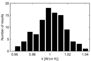
Figure 4: Distribution of conductivity values when synthetic, normally distributed noise with $\sigma$ = 1 mK is added to a synthetic data set. The mean value is $(1.001\pm 0.017)$ $\mbox{W}/(\mbox{m K})$.

3 Calculation of errors

For inversions theoretical errors can be calculated using the model kernel ${\bf G}$ (Menke,, 1989):

$$\bf cov_{m}=G^{-I}cov_{d}G^{-IT}$$ (19)

Here ${\bf cov_{m}}$ and ${\bf cov_{d}}$ are the covariance matrices of the model parameters and the data, respectively. ${\bf G^{-I}}$ is the inverse of the kernel, in our case ${\bf VS^{-1}U^{T}}$ (equation 15). This equation is only exact for linear problems with normally distributed data. Nevertheless, it can be applied to a nonlinear problem, if the problem can be approximated by a linear function in the vicinity of the solution. It is a useful property of equation 19 that no data is used for the calculation of errors, only the data covariance and a model kernel are needed. The kernel can be computed using equation 12 by assuming a parameter vector with representative values. This choice is not critical since the kernel and corresponding errors vary only slowly with the parameters. This feature of equation 15 is particularly useful for design studies and theoretical evaluation of the limitation of a certain model.

The covariance matrix of the data is not known a priori but in our case it can be assumed that data errors are uncorrelated and mainly due to the finite temperature resolution of $\pm$1 mK. ${\bf cov_{d}}$ is then a matrix with temperature variances on its main diagonal and zeros elsewhere. To compute the kernel ${\bf G}$ using equation 12, a modelled decay curve from 120–420 s with 10 s sampling rate and two sets of parameters for frictional and heat pulse decay are used, respectively. These values, together with the calculated errors, are summarised in table 2. For the frictional decay, errors for $Q,t_{s}$ and $T_{a}$ are determined, according to the processing sequence given in section 2. The ambient temperature can be resolved with a standard deviation of 1.4 mK, or with a relative error of 0.28%. For the heat pulse decay, errors for $k,\kappa$ and $t_{s}$ were computed. The standard deviation of the thermal conductivity is 0.018  $\mbox{W}/(\mbox{m K})$ (1.8%).

The error bounds given in table 2 give a general idea of the errors to be expected when using the algorithm. The relevant parameters conductivity and sediment temperature can be calculated with relative errors of about 2.0 and 0.5%, respectively. For the parameter range encountered in practice, errors will vary slightly. Therefore, for each penetration errors are calculated from the inversion results and stored together with them.

4 Tests of the proposed inversion scheme

To verify the theoretically derived error bounds, normally distributed noise with $\sigma$ = 1 mK was added to the exact model data. This data was then inverted. To obtain reasonable statistics the procedure was repeated 100 times, producing results for $k$ which are shown in the histogram in Figure 4. The mean of the computed conductivities, (1.001$\pm$0.017) $\mbox{W}/(\mbox{m K})$, agrees very well with the expected value of (1.00$\pm$0.018) $\mbox{W}/(\mbox{m K})$.

The value of ${(\rho c)_{c}}$ is only known on the basis of geometric considerations (Nagihara & Lister,, 1993). Additionally, its value could vary by a few percent over the length of the sensor string because of more wiring in the upper parts of the string. If a wrong value for ${(\rho c)_{c}}$ is assumed it will influence the results of the inversion in a systematic way. Therefore it is useful to investigate the magnitude of the error introduced by an incorrect value.

Figure 5: Influence of false ${(\rho c)_{c}}$-values on inversion results. Variations of up to 15% result in no significant change in $k$.

A synthetic temperature record was calculated using the same parameters as in the previous section. ${(\rho c)_{c}}$ was chosen to be 3.38 $\cdot 10^{6}\mbox{ J}/(\mbox{K m}^{3})$, the value given by Nagihara & Lister, (1993). This record was the input to an inversion in the heat pulse-configuration ($k$, $\kappa$, $t_{s}$ are calculated). Several runs were made, each time with a slightly different value for the heat-capacity, ranging from 2.9 to 3.9$\cdot 10^{6}\mbox{ J}/(\mbox{K m}^{3})$which corresponds to a relative deviation of about $\pm$15%.

Figure 5 shows relative errors in the calculated model parameters when ${(\rho c)_{c}}$ is varied. For the maximum bias, the deviation of the conductivity is only about 0.2%. This value is considerably smaller than the errors introduced from other sources.

The situation is different for the other two parameters though. The systematic deviations are significant compared to the random errors. $t_{s}$ only has meaning within the framework of the inversion algorithm, but $\kappa$ is a physical parameter and a relationship based on the calculated $\kappa$ could be in error by a few percent.

The tests were conducted using synthetic data based on equation 6. A time shift can be computed for model curves but it cannot be verified whether $t_{s}$ is able to approximate the non-ideal parts of real temperature records.

A closer approximation to reality is a numeric model that is able to model finite heat pulse length and finite probe conductivity. For this reason a program called TFELD was used which is based on an algorithm proposed by Villinger, (1985). This program allows modelling of heat diffusion in a cylindrically layered space with various heating functions. Each of the cylindrical layers is characterised by a set of physical parameters $\rho$, $k$ and $c$. In this case a model with only two layers was employed, the inner and the outer layer representing the probe and the sediment, respectively.

In the first model used the conductivity and diffusivity of the probe (layer 1) were set to 1000 $\mbox{W}/(\mbox{m K})$ and 2000$\cdot 10^{-7}\mbox{ m}^{2}/\mbox{s}$ respectively to give a good approximation of an ideal probe. The ambient sediment (layer 2) values of 1 $\mbox{W}/(\mbox{m K})$ and 2$\cdot 10^{-7}\mbox{ m}^{2}/\mbox{s}$ were used as representative values for conductivity and diffusivity. An instantaneous temperature rise of the inner cylinder was used as the heat source. The computed temperature decays were used as input for the inversion algorithm. The results are shown in table 3.

		TFELD	T2C
$k$	$\left[\frac{\mbox{ W}}{\mbox{m K}}\right]$	1.0	1.0002
$\kappa$	$\left[10^{-7}\frac{\mbox{ m}^{2}}{\mbox{ s}}\right]$	2.0	2.0019
$t_{s}$	[s]	0.0	0.0016

Table 3: Inversion results of the TFELD model. The results show good agreement.

As expected the inversion gives the correct result within the precision of the numerical computations.

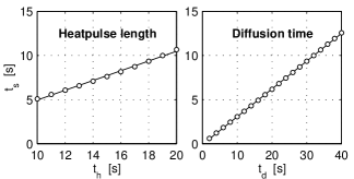
Figure 6: Influence of non ideal probe parameters: a) finite heating b) finite diffusivity.

The main objective of using the TFELD model was to study the influence of a non-ideal probe on the temperature decay curves. In the literature (Hyndman et al.,, 1979; Villinger & Davis,, 1987; Nagihara & Lister,, 1993) it is assumed that the effects of the finite thermal conductivity of the cylinder and the finite heat pulse on the temperature decay will be combined in the time shift $t_{s}$.

In order to separate effects of finite heating and probe geometry two experiments were conducted, one with an approximately ideal probe and finite heat pulse and a second with real probe geometry and infinitely short heat pulse.

For the first experiment probe conductivity was fixed at 1000 $\mbox{W}/(\mbox{m K})$ and heat pulses with duration from 10–20 s were used as input to TFELD. The resulting decay curves were inverted using T₂C. If the time shift from the inversion is plotted versus the length of the heat pulse (Figure 6a), a strong linear relationship can be seen.

A similar test was run to determine the relationship between probe geometry and time shift. It was found that the parameter suited best to describe the probe geometry is the diffusion constant $t_{d}$:

$$t_{d}=\frac{a^{2}}{\kappa}$$ (20)

This value describes the time that a temperature disturbance would take to travel the distance $a$. The diffusion time of the probe was varied from 2–40 s in this experiment corresponding to values for $k$ and $\kappa$ of 40–2  $\mbox{W}/(\mbox{m K})$ and 80–4 $\cdot 10^{-7}\mbox{ m}^{2}/\mbox{s}$, respectively. The initial temperature field was $T_{0}$ inside the probe and zero outside. Again these model curves were inverted and the resulting time shifts plotted versus the diffusion time to obtain the linear relationship seen in Figure 6b.

If a linear fit is calculated for both curves, the following relationships are obtained:

$$t_{s}=0.55t_{h}-0.56\,\qquad\mbox{[s]}$$ (21)

$$t_{s}=0.31t_{d}-0.08\,\qquad\mbox{[s]}$$ (22)

Here $t_{h}$ is the duration of the heat pulse. It is intuitively explicable that a temperature record, generated by a finite heat pulse can be best described by a perfect pulse shifted half the length of the original pulse. Similarly the probe geometry will result in a time shift that is directly dependent on the time the heat pulse needs to travel through the internal structure. This is reflected in equations 21 and 22, respectively.

One reason for the development of our algorithm was to evaluate the possibilities of calculating the conductivity directly from the frictional decay. In this case the only known parameter is $(\rho c)_{c}$. From the discussion of the spectrum of the SVD, it is clear that a reduction of the number of parameters to at least four is necessary to invert equation 1 as an overdetermined problem. To reduce the number of parameters in the problem by one, a relationship between conductivity and diffusivity can be used (Hyndman et al.,, 1979).

$$\kappa=\frac{k}{5.79-3.67k+1.016k^{2}}\qquad\left[10^{-6}\frac{\mbox{m}^{2}}{\mbox{s}}\right]$$ (23)

This assumption is justified because both conductivity and diffusivity of marine sediments are mainly porosity controlled. Using equation 19 one can calculate expected error bounds for this configuration. If an observational error of $10^{-3}$ K and reasonable parameters for probe and sediment are assumed, the errors in the model parameters are as follows:

• $\Delta k$ = 6.6 $\mbox{W}/(\mbox{m K})$

• $\Delta Q$ = 1500$\mbox{ J}/\mbox{ m}$

• $\Delta t_{s}$ = 58 s

• $\Delta{T_{a}}$ = 12 mK

It can be seen in equation 19 that the model covariance is linearly related to the data covariance. If an error margin of $0.05\leavevmode\nobreak\ \mbox{W}/(\mbox{m K})$ ($\approx\pm 5$ % for marine sediments) is assumed as an acceptable error level for the conductivity, this means a reduction of $\Delta k$ by 2 orders of magnitude. This means as well a reduction of the observational error by 2 orders of magnitude. Thus, accuracy of temperature readings has to be reduced to an extremely low and unrealistic level of $\pm 10^{-5}$ K. The results of these tests confirm that the frictional decay is not sensitive to the thermal conductivity of the surrounding sediment and a successful inversion for $k$ with realistic error bounds for the temperature measurements is not possible.

The reason for this failure is implicit in the model. Not enough information is provided by a frictional decay curve to resolve the ambiguity of the problem using an inversion scheme. Programs exist, however, that are capable of modelling the full frictional decay (forward modelling), including the early times (Lee & Von Herzen,, 1994; Villinger,, 1985). This allows other constraints to be added to the problem, thereby reducing the ambiguity (Lee & Von Herzen,, 1994). It has to be considered, however, that any additional assumptions and a-priori information will directly affect computation of thermal conductivities and have to be chosen carefully.

Thermal parameters:
Conductivity	(1.609 $\pm$ 0.016) $\mbox{W}/(\mbox{m K})$
Diffusivity	7.3$\cdot 10^{-7}\mbox{ m}^{2}/\mbox{s}$
Heat capacity	2.20$\cdot 10^{6}\mbox{ J}/(\mbox{K m}^{3})$
Measurement parameters:
Heating power	8, 12, 15$\mbox{ W}/\mbox{ m}$
Heat pulse duration	5, 10 s
Sampling rate	0.5 s
Observational error	10-4 K

Table 4: Upper half: Thermal parameters of the material used for needle-probe measurements. Lower half: Parameters of the different records taken.

5 Inversion of needle-probe measurements

To test the algorithm with real data, a set of pulsed needle-probe measurements were used. These were made in a ceramic alloy with a known thermal conductivity close to the value of deep sea sediments. The data were kindly provided by TeKa Inc. (Berlin, Germany), a company specialised in thermal conductivity measurements and equipment. The true conductivity of the ceramics was measured with a divided bar device (TeKa Inc., pers. comm.). The relevant parameters of the material and the recording settings are summarised in table 4. For each combination of parameters three decay curves were recorded, resulting in a total of 18 decay curves.

A drift correction was applied to the temperature records to reduce the value of the ambient temperature ${T_{a}}$ to zero. The heat capacity of the probe was unknown so that the decay curves were inverted using four unknown parameters: $[k,\kappa,{(\rho c)_{c}},t_{s}]$. The results for the conductivity with 1-$\sigma$ error bars are shown in figure 7. The circles represent the computed thermal conductivities together with 1-$\sigma$ error bars. The dashed lines are the mean thermal conductivity and 1% error margins determined with the divided bar method. Shown are all 18 measurements in six groups of three measurements with the same heating parameters. On the top horizontal axis, the heating parameters are encoded in the names: The first two digits represent the duration [s], the last two digits the heating power per unit length [W/m] of the heat pulse. For each set of parameters, three measurements were made.

Figure 7: Inversion results for the needle-probe measurements. The circles represent calculated conductivities with 1-$\sigma$ error bars for the 18 records.

There is excellent agreement between expected and calculated values of the heat conductivity. Errors of $k$ were between 0.2 and 0.5%. For the $\kappa$-values the errors are 3–15% and for $(\rho c)_{c}$ 10–30%. The high accuracy of the conductivity value compared to previous tests is due to the small observational error of the needle probe. As stated before, large errors for $\kappa$ and $(\rho c)_{c}$ are related to the inversion with four unknown parameters.

The error bounds generally decrease to the right in figure 7. Changes in length of the heat pulse and heating power affect the total heat input and the recorded temperature signal. Thus it appears that calculated error bounds vary with the magnitude of the recorded temperature changes, as expected.

It is interesting to check whether the hypothesis that the time shift is connected to the diffusion time via a simple relationship of the type in equation 21 holds true for real data. Figure 8 shows that all $t_{s}$ fall into two clearly distinguishable groups according to the duration of the heat pulse (5 and 10 s). The difference of about 2.5–3.0 s is in good agreement with the expected value, which should be half the difference of the lengths of the heat pulses.

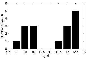
Figure 8: Distribution of calculated time shifts for the needle-probe measurements. Two clearly distinguishable groups can be identified that are about 2.5 s apart from each other.

6 Results from research cruise SO111

During summer of 1996 cruise SO111 was conducted off Western Canada on the German research vessel SONNE. The objective was to study the effect of hydrothermal circulation on marine heat flow on the Eastern flank of the Juan de Fuca Ridge. The survey area was located near the Cobb Offset at about 47^∘ 30’ N, 129^∘ 0’ W. During the cruise 8 stations with 104 successful penetrations were made. For a detailed discussion of the measurements during this cruise see Villinger & Fahrtteilnehmer, (1996).

This cruise provided the first instance to use the program on a regular basis. The following is concerned mainly with the application of the inversion algorithm. Though all penetrations were inverted successfully using the described algorithm only data from station 2 with 30 penetrations will be used to illustrate the applicability of the program.

In the first stage of processing the moment of penetration of the probe and the onset of the heat pulse have to be picked manually using the raw temperature data. The data can then be input to the inversion program that calculates thermal parameters according to the previously described sequence. The thermal parameters are then in turn used to calculate heat flow values.

To minimise the influence of the non-ideal probe at early times, only temperatures for times $>$ 120 s relative to the picked origin time were used. The value for this start time depends on the probe geometry and was found empirically by examining the fit for several start times. For example Nagihara & Lister, (1993) used a sensor string with a diameter of 9.52 mm versus 8.0 mm in our design and a value of 200 s as the starting time for their analysis.

After calculation of conductivities and thermal gradient, the absolute penetration depth can be calculated using the bottom water temperature and the assumption that the temperature is continuous at the sediment-water interface. Figure 9 shows the conductivity versus the sensor depth for station 2. A strong increase in conductivity over the first metre can be seen that is possibly caused by a decrease of porosity in the surface sediments. The outliers in the lower part of the plot might be attributed to a partially penetrated sand layer of varying depth. This corresponds to the observation that often the penetration was stopped by a layer of harder material.

Figure 9: Conductivity-depth profile for station 2.

Previous workers (Bullard, (1954); Ratcliffe, (1960); Von Herzen & Maxwell, (1959); Hyndman et al., (1979)) determined thermal diffusivity by measuring conductivity, density and porosity. Assuming that heat capacity and conductivity are controlled mainly by the water content, they constructed a relationship between thermal conductivity and diffusivity. In our approach, thermal diffusivity is computed as an independent parameter in the inversion. Figure 10 shows calculated diffusivity values compared to the relationship (Equation 23) given by Hyndman et al., (1979). The inversion results are significantly lower than expected by the theoretical curve. To our knowledge no other measurements of our type for marine sediments are published to verify the results. It is apparent, though, that a simple equation is not sufficient to describe the variations in the relation between $k$ and $\kappa$.

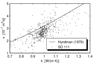
Figure 10: Calculated diffusivity versus conductivity for station 2. The values are compared to an empirical relationship by Hyndman et al., (1979).

It is instructive to compare the results of HFRED (Villinger & Davis,, 1987) to our results. Figure 11 shows differences in computed conductivity for both algorithms. A high agreement is visible with deviations usually within $\pm$5%.

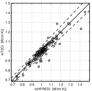
Figure 11: Comparison of thermal conductivities between T₂C described in this paper and HFRED (Villinger & Davis,, 1987). Dashed lines show a relative deviation of $\pm$ 5%.

HFRED uses a constant value for the ratio of the heat capacities $\alpha$ of 2.0 because of the lack of knowledge of the thermal diffusivity. In the T₂C algorithm $\alpha$ is not used but can be calculated from the computed thermal diffusivity as $\kappa=k/{(\rho c)_{c}}$. Figure 12 shows relative differences of the thermal conductivity versus $\alpha$. It is apparent that large deviations from $\alpha=2$ correspond to large differences in thermal conductivity, suggesting that a constant value of $\alpha$ is not sufficient to describe all measurements accurately.

7 Conclusion

An algorithm is described to invert heat flow measurements made with a violin-type heat probe including in-situ thermal conductivity measurements after the pulse method of Lister, (1970). A theoretical analysis of the inversion algorithm shows that undisturbed sediment temperatures can be determined with an error of about 1–2 mK. The absolute error of the in situ thermal conductivity $k$ is less than 0.002  $\mbox{W}/(\mbox{m K})$. It is also possible to compute thermal diffusivities, but with considerably higher errors of about 10 %.

Numerical experiments with synthetic temperature decay data reveal a strong relationship between the time shift and the thermal probe parameters which can be explained in a quantitative way by the finite length of the heat pulse and the diffusion time constant of the sensor string.

Measured data, obtained with a needle probe in material with known thermal conductivity, confirm the accuracy of the inversion procedure and show that the algorithm is suited to the analysis of pulsed needle probe measurements. Our results show that is is possible to succesfully use the algorithm in pulsed needle probe measurements.

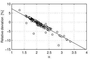
Figure 12: Relative differences of conductivities computed with HFRED and T₂C as a function of $\alpha$.

The inversion of the data obtained on SO111 proves that the described algorithm is robust and well suited for automated processing of a large number of heat flow penetrations. The embedding of the software in a suite of mathematical software allows simple further analysis of the data and easy development of additional tools. The relative accuracy of our thermal conductivity results is in the range of 1–3%. Undisturbed sediment temperatures can be computed with relative errors of 0.5–1%. The comparison with results obtained with the previously used program HFRED (Villinger & Davis,, 1987) shows good agreement between both algorithms. Deviations are generally due to the assumption of $\alpha=2$ by HFRED.

References

- Bullard, (1939) Bullard, E. C., 1939. Heat flow in South Africa, Proc. R. Soc. London, Series A, 173, 474–502.
- Bullard, (1954) Bullard, E. C., 1954. The flow of heat through the floor of the atlantic ocean, Proc. R. Soc. London, Series A, 222, 408–425.
- Carslaw & Jaeger, (1959) Carslaw, H. S. & Jaeger, J. C., 1959. Conduction of heat in solids, Oxford University Press, 2nd edn.
- Hyndman et al., (1979) Hyndman, R. D., Davis, E. E., & Wright, J. A., 1979. The measurement of marine geothermal heat flow by a multipenetration probe with digital acoustic telemetry and in situ thermal conductivity, Mar. Geophys. Res., 4, 181–205.
- Jones, (1999) Jones, E. J. W., 1999. Marine Geophysics, Wiley, Chichester, UK.
- Kristiansen, (1982) Kristiansen, J. I., 1982. The transient cylindrical probe method for determination of thermal parameters of earth materials, GeoSkrifter 18, Laboratory of Geophysics, Aarhus, Denmark.
- Lee & Von Herzen, (1994) Lee, T.-C. & Von Herzen, R. P., 1994. In situ determination of thermal properties of sediments using a friction-heated probe source, J. Geophys. Res., 99(B6), 12121–12132.
- Lister, (1970) Lister, C. R. B., 1970. Measurement of in situ sediment conductivity by means of a Bullard-type probe, Geophys. J. R. astr. Soc., 19, 521–532.
- Lister, (1979) Lister, C. R. B., 1979. The pulse-probe method of conductivity measurement, Geophys. J. R. astr. Soc., 57, 451–461.
- Menke, (1989) Menke, W., 1989. Geophysical Data Analysis: Discrete Inverse Theory, no. 45 in International Geophysics Series, Academic Press, rev. edn.
- Nagihara & Lister, (1993) Nagihara, S. & Lister, C. R. B., 1993. Accuracy of marine heat-flow instrumentation: Numerical studies on the effects of probe construction and the data reduction scheme, Geophys. J. Int., 112, 161–177.
- Ratcliffe, (1960) Ratcliffe, E. H., 1960. The Thermal Conductivity of Ocean Sediments, J. Geophys. Res., 65(5).
- Villinger, (1985) Villinger, H., 1985. Solving cylindrical geothermal problems using the Gaver-Stehfest inverse Laplace transform, Geophysics, 50(10), 1581–1587.
- Villinger & Davis, (1987) Villinger, H. & Davis, E. E., 1987. A New Reduction Algorithm for Marine Heat Flow Measurements, J. Geophys. Res., 92(B12), 12846–12856.
- Villinger & Fahrtteilnehmer, (1996) Villinger, H. & Fahrtteilnehmer, 1996. Fahrtbericht SO111, Berichte aus den Geowissenschaften 97, Universität Bremen.
- Von Herzen & Maxwell, (1959) Von Herzen, R. & Maxwell, A. E., 1959. The Measurement of Thermal Conductivity of Deep-Sea Sediments by a Needle-Probe Method, J. Geophys. Res., 64(10), 1557–1563.