A large N phase transition in the continuum two dimensional SU(N) X SU(N) principal chiral model.

Abstract:

It is established by numerical means that the continuum large N principal chiral model in two dimensions has a phase transition in a smoothed two point function at a critical distance of the order of the correlation length.

1 Introduction.

It is well known that the principal chiral $SU(N)\times SU(N)$ model (PCM) in two Euclidean dimensions is similar to four dimensional pure $SU(N)$ gauge theory in many respects [1].

Recent numerical work provides evidence that Wilson loops in $SU(N)$ gauge theory in two, three and four dimensions exhibit an infinite $N$ phase transition as they are dilated from a small size to a large one; in the course of this dilation the eigenvalue distribution of the untraced Wilson loop unitary matrix expands from a small arc on the unit circle to encompassing the entire unit circle [2, 3]. There is further evidence that in the vicinity of the critical size and for eigenvalues close to -1, the eigenvalues behave in a universal manner controlled by two critical exponents of $N$, taking the values 1/2 and 3/4. The universality class of this transition is believed to be that of a random multiplicative ensemble of unitary matrices. The transition was discovered by Durhuus and Olesen [4] when they solved the Migdal-Makeenko [5] loop equations in two dimensional planar QCD. We refer to it therefore as the DO transition and to the universality class as the DO class. The multiplicative random matrix ensemble [6] can be axiomatized in the language of noncommutative probability [7]. In some sense it provides a generalization of the familiar law of large numbers, which is associated to the abelian case. The essence of the difference is not in that the law of large numbers is additive, while the new case is multiplicative; rather, the essential features making a difference are that one case is commutative and the other not. Various recent insights into the DO transition  [8, 9, 10] indicate that an even deeper understanding of the transition might emerge.

In this work we present numerical results indicating that the PCM model has a similar transition, this time in the two point correlator matrix: when it is dilated it undergoes a DO transition. Thus, the analogy between the PCM and gauge theory is upheld and the universal character of the DO transition as a marker for the transition scale separating weakly from strongly interacting dynamics in theories based on group manifolds is expanded.

2 Basic facts about the PCM.

The basic degrees of freedom are $g(x)\in SU(N)$ where $x\in R^{2}$ and the action is:

$$S=\frac{N}{T}\int d^{2}xTr\partial_{\mu}g(x)\partial_{\mu}g^{\dagger}(x)$$ (1)

The large $N$ limit is taken in the ’t Hooft prescription, by keeping the coupling $T$ fixed, which makes $S$ of naive order $N^{2}$.

There is a global symmetry group $SU(N)_{L}\times SU(N)_{R}$ acting on $g(x)$ by $g(x)\rightarrow Lg(x)R^{\dagger}$ where $L,R\in SU(N)$. If we eliminate one of the factors by a translation breaking “gauge choice” $g(0)=1$, we are left with a global symmetry given by a single $SU(N)$ acting on $g(x)$ by conjugation and leaving $g(0)=1$ unchanged. This single $SU(N)$ is the “diagonal subgroup” of the global symmetry group.

The model is asymptotically free and has a nonzero massgap. Using Bethe ansatz methods it was found that there are $N-1$ particle states with masses given by

$$M_{r}=M\frac{\sin(\frac{r\pi}{N})}{\sin(\frac{\pi}{N})},~{}~{}~{}1\leq r\leq N-1$$ (2)

Under the diagonal symmetry group, the states corresponding to the $r$-th mass are a multiplet transforming as an $r$ component antisymmetric tensor. This has been verified numerically for $N=6$ in [11]. In consequence it is believed that for any $N$ and $1\leq r\leq N-1$ we would have

$$\langle\chi_{r}(g(0)g^{\dagger}(x))\rangle\sim C_{r}{N\choose r}e^{-M_{r}|x|}$$ (3)

for $|x|M>>1$. Here, $\chi_{r}$ takes the trace in the $r$-antisymmetric representation, normalized by $\chi_{r}(1)={N\choose r}$.

The PCM can be formulated in terms of the currents $J_{\mu}(x)=g^{\dagger}(x)\partial_{\mu}g(x)$. Note that the object $g(0)g^{\dagger}(x)$ is determined by the $J_{\mu}$ via a path ordered exponent. In particular, also the action can be expressed in terms of the $J_{\mu}(x)$. In addition, the $J_{\mu}(x)$ obey local constraints because if viewed as gauge fields they are pure gauge.

3 The average characteristic polynomial and the DO transition.

It was found that a convenient observable to use in order to locate the DO transition and identify the associated critical $N$-exponents is provided by the average characteristic polynomial of the unitary matrix undergoing the transition. This matrix is the open Wilson loop in the gauge case while in the PCM model it is $g(0)g^{\dagger}(x)$.

For gauge theory in two dimensions, for a non-self-intersecting loop, the unitary matrix can be written as the product of many such open Wilson loop matrices round small loops tessellating the spanning area of the loop. For a gauge theory in higher dimensions we choose an infinite two dimensional surface extending to infinity and containing the loop in question and repeat the argument for gauge fields tangent to the surface. The DO transition occurs because for large loops the correlations between well separated tessellating loops die out and the factors become effectively independent. In two dimensions any two distinct tessellating loops are uncorrelated. Note that the “number” of factors in the product is proportional to the area enclosed by the loop; this product is not to be identified with the linearly ordered product associated with the path ordered exponential.

For the PCM, we split the segment connecting $0$ to $x$ into small intervals, with $J_{\mu}(y)$ determining a multiplicative contribution for each element. Again, for large $|x|$, the correlations between well separated small intervals dies out, and a DO transition might occur. This time however, the “number” of factors is proportional to the linear distance $|x|$. Again, this random product is not to be identified with the product between the two matrices in the two-point correlation function. And, yet again, if we descend in dimensions (here to one dimension) any two distinct intervals are uncorrelated and the DO transition can be established by an exact analytical solution.

In either case, gauge or PCM, if $W$ is the unitary matrix given by the product of independent factors, the average characteristic polynomial is defined in the same manner:

$$Q_{N}(z,\lambda)\equiv\langle\det(z-W)\rangle=\sum_{r=0}^{N}z^{N-r}(-1)^{r}\langle\chi_{r}(W)\rangle$$ (4)

Here $\lambda$ is a continuous parameter which has been kept finite by tuning the distribution of the individual factors in the product to almost always produce something finite after multiplying the many factors. In a sense, $\lambda$ would measure the area in the gauge case and the distance in the PCM case. In general, one can view $\lambda$ as a parameter quantifying the amount of dilation of the object relative to a fixed standard.

In the simple case of two dimensional gauge theory one can take $\lambda$ to be literally the area, made dimensionless with the aid of the coupling constant, and the DO transition can be seen when one uses

$$\langle\chi_{r}(W)\rangle={N\choose r}e^{-\lambda\frac{r(N-r)}{2N}}$$ (5)

For the PCM, we expect,

$$\langle\chi_{r}(W)\rangle\sim C_{r}{N\choose r}e^{-M|x|\frac{\sin(\frac{r\pi}{N})}{\sin(\frac{\pi}{N})}}$$ (6)

We observe that the exponents in the gauge and PCM case are similar, with $M|x|$ playing the role of $\lambda/2$. More precisely, for $r=O(1)$ or $N-r=O(1)$ and large $N$ they match and for $r\sim N$ they do no differ that much. Thus, if the coefficients $C_{r}$ vary less than the other factors, the singularity structure at a critical value of $\lambda$ in the infinite $N$ limit would be the same. We conclude that the PCM model could also exhibit the DO transition. It would be nice to confirm this by exact analytical methods, in particular since the numerical work we shall present indicates that the DO transition does occur in the PCM. The commonality between the gauge and PCM case exponents is related to a topic known as “Casimir scaling”.

4 Regularization and renormalization.

Until now we ignored renormalization. In both the gauge and PCM case one needs to renormalize and there is no guarantee that after that it makes sense to view $W$ as a fluctuating unitary matrix of unit determinant. Formally, we can define a renormalized version of the $W$ matrix in each case which does provide for such a view. The gauge case was analyzed in other work, so from now on we restrict ourselves to the PCM case.

The extra regularization we put in is of the operator. The action is regularized with appropriate counter terms in some conventional manner. The net (formal) result is that we assume that we have a probability distribution generating “bare” configurations $g_{0}(x)$.

Let $\tau\geq 0$ be a parameter of dimension length squared which means that $\tau M^{2}$ is a finite unitless parameter. We extend $R^{2}$ (space time) by an $R^{+}$ coordinated by $\tau$ and define a $g(x,\tau)$ determined by $g_{0}(x)$ by:

$$g^{\dagger}(x,\tau)\frac{\partial g(x,\tau)}{\partial\tau}=\frac{1}{2}[\partial^{2}g(x,\tau)-\partial^{2}g^{\dagger}(x,\tau)]-\frac{1}{2N}Tr[\partial^{2}g(x,\tau)-\partial^{2}g^{\dagger}(x,\tau)]$$ (7)

with the initial condition

$$g(x,0)=g_{0}(x)$$ (8)

The evolution in $\tau$ ensures that $g(x,\tau)\in SU(N)$ if $g_{0}(x)\in SU(N)$. For $g(x,\tau)=e^{iB(x,\tau)}$ with $TrB(x,\tau)=0$ and $||B||<<1$ the equation becomes

$$\frac{\partial B(x,\tau)}{\partial\tau}\approx\partial^{2}B(x,\tau)$$ (9)

This shows that for $\tau>0$ high momentum modes will get suppressed. $g(x,\tau)$ depends nonlocally on $g_{0}(y)$; the amount of nonlocality is characterized by the unitless finite quantity $\tau M^{2}$, which is parametrically small relative to one, but nonzero. As a result, the correlation function $\langle g(x,\tau)g^{\dagger}(y,\tau)\rangle$ will stay finite and nontrivial in the continuum limit so long as $\tau>0$ without needing the extraction of wave function renormalization factors.

Hence, the $SU(N)$ matrix $W$ we shall compute the average characteristic polynomial of will depend on an extra parameter $\tau>0$. The critical scale $|x-y|_{c}$ will have some weak dependence on $\tau$. The point is that so long as $\tau M^{2}$ is parametrically small relative to unity, there will be some finite $|x-y|_{c}$ where the transition occurs, but the exact value of that $|x-y|_{c}$ is renormalization dependent. The relevant fact is that the DO transition occurs somewhere and there it marks a sharp boundary separating strong and weak couplings as defined from this particular two point function.

5 Lattice formulation.

The continuum formulation ended up with three continuum coordinates. We now discretize each. The two dimensional space-time becomes a square lattice with unit lattice spacing, whose sites are again denoted by $x$, with $x\in Z^{2}$. $\pm\mu$ denote unit vectors in the positive/negative $\mu=1,2$ direction. The $\tau$ direction becomes a unit spaced line labeled by a coordinate $t=0,1,2,...$. The variables that enter the action are $g(x)\in SU(N)$ and the $\tau$-dependence of the smeared variables is denoted by $g_{t}(x)$, with $g_{0}(x)=g(x)$. The system is made finite by taking the $x$-space to be a torus lattice of equal side lengths, $L$. The extent in the $\tau$ direction is $n$. Only the space-time direction is stored in the computer, while the $t$ dependence is iteratively computed. The $g(x)$ obey periodic boundary conditions and $g_{t}(x)$ for $t=1,2,...,n$ is determined by $g(x)$ in a manner preserving this.

The lattice action is:

$$S_{L}=-2Nb\sum_{x,\mu}\Re Tr[g(x)g^{\dagger}(x+\mu)]$$ (10)

Averages with respect to

$${\cal N}\prod_{x}[dg(x)]e^{-S_{L}}$$ (11)

are denoted by $\langle...\rangle$ where ${\cal N}$ is a normalization constant ensuring $\langle 1\rangle=1$. Thus, the two point function is

$$G(x)=\frac{1}{N}\langle Tr[g(0)g^{\dagger}(x)]\rangle$$ (12)

When $N$ is taken to $\infty$ with $b$ fixed (this is the ’t Hooft large $N$ limit) $G(x)$ remains a finite nontrivial function of $x$. In particular, $\xi_{G}$, defined below, measures the correlation in lattice units.

$$\xi_{G}^{2}=\frac{1}{4}\frac{\sum_{x}x^{2}G(x)}{\sum_{x}G(x)}$$ (13)

$\xi_{G}$ is independent of the wave function renormalization constant. It sets the scale for the system in units of the lattice spacing. The continuum limit is obtained when $b$ is taken to infinity, which causes $\xi_{G}$ to diverge.

It has been found that [11] (a number further improved in subsequent work) that in the continuum one has

$$M\xi_{G}=0.991(1)$$ (14)

Here, $M$ is the lattice equivalent of the continuum mass $M=M_{1}$ from Equation (2). We shall use $\xi_{G}$ as the scale setting quantity.

The extrapolation to infinite $b$ is greatly helped by using $E$, the link energy, as an expansion parameter:

$$E=1-\frac{1}{N}\Re\langle Tr[g(0)g^{\dagger}({\hat{1}})]\rangle$$ (15)

As $b\to\infty$, $E\to 0$. This scheme is equivalent to what is also known as “mean field improvement”. In the range we shall be working and setting $N$ to infinity, the following formula translates $E$ into $b$ to high enough accuracy:

$$E=\frac{1}{8b}+\frac{1}{256b^{2}}+\frac{0.000545}{b^{3}}-\frac{0.00095}{b^{4}}+\frac{0.00043}{b^{5}}$$ (16)

The following formula is found to work within a few percent in the range we shall be working in, which is $11\leq\xi_{G}\leq 20$. Again, we use the $N=\infty$ expression, but know that $\frac{1}{N^{2}}$ corrections are small.

$$\xi_{G}=0.991~{}\left[\frac{e^{\frac{2-\pi}{4}}}{16\pi}\right]~{}\sqrt{E}~{}\exp\left(\frac{\pi}{E}\right)$$ (17)

Using this formula as setting the scale for all dimensionful physical quantities, the approach to continuum can be tested to a level below one percent.

The smearing operation is discretized as follows: We start from a configuration $g(x)\equiv g_{0}(x)$ and evolve with a fixed smearing parameter $0<f<<1$ to a configuration $g_{t}(x)$. One smearing step takes us from $g_{t}(x)$ to $g_{t+1}(x)$. We first define $Z_{t+1}(x)$ by:

$$Z_{t+1}(x)=\sum_{\pm\mu}[g^{\dagger}_{t}(x)g_{t}(x+\mu)-1]$$ (18)

Next we construct antihermitian traceless $SU(N)$ matrices $A_{t+1}(x)$

$$A_{t+1}(x)=Z_{t+1}(x)-Z^{\dagger}_{t+1}(x)-\frac{1}{N}\rm{Tr}(Z_{t+1}(x)-Z^{\dagger}_{t+1}(x))\equiv-A^{\dagger}_{t+1}(x)$$ (19)

and set

$$L_{t+1}(x)=\exp[{fA_{t+1}(x)}]$$ (20)

Finally, $g_{t+1}(x)$ is defined in terms of $L_{t+1}(x)$ by:

$$g_{t+1}(x)=g_{t}(x)L_{t+1}(x)$$ (21)

This procedure is iterated until $t=n$ is reached. Each iteration is performed for all $x$ and only then one goes to the next iteration.

For a given $\xi_{G}$ (or $b$) the parameter $\tau$ is fixed keeping the quantity $\tau/\xi_{G}^{2}$ unchanged; here, $\tau=nf$ is in units of lattice spacing. Again, $\tau$ is the lattice analogue of the continuum parameter $\tau$. Within our range of parameters and with our choice for $\tau/\xi_{G}^{2}$ we found that it is enough to set $n=30$ in order to eliminate a visible dependence on the two factors $f$ and $n$ individually, making only $fn$ relevant. This ensures that when extrapolating to the continuum limit by increasing $\xi_{G}$ we eliminate sensitivity on the discretization of the smearing process.

The set of matrices $g(x)$ is generated by Monte Carlo for the action $S_{L}$. We set $\xi_{G}$ and obtain the corresponding $b$. We use a combination of Metropolis and Over-Relaxation at each site $x$, where we explore the full $SU(N)$ group. Thus, the operation count goes as $N^{3}$ for generating configurations. We found that 200-250 passes suffice to thermalize the system starting from $g(x)\equiv 1$. When going from a configuration with some $\xi_{G}$ to another with $\xi_{G}$ increased by 1, 50 passes are enough for equilibration and approximate statistical independence.

One major difference between gauge theories [12, 13] and the PCM in the context of the large $N$ limit is that in the PCM there is no special suppression of finite volume effects. From previous numerical work on the PCM we know that keeping $L/\xi_{G}>7$ reduces finite volume effects to below one percent. As already mentioned, we carry out simulations in the range $11\leq\xi_{G}\leq 20$. Therefore we chose $L=150$, a relatively large box-size. For smearing we chose

$$\tau=\frac{\xi_{G}^{2}}{300}$$ (22)

This is a small amount of smearing, but some smearing is necessary in the continuum limit because we need to avoid the short distance singularity one would otherwise expect. A singularity is incompatible with the $W$ matrices being unitary, and hence bounded, in the continuum limit,

For each $g(x)$ we generate we compute matrices

$$W_{\mu}(d)=g_{n}(x)g^{\dagger}_{n}(x+d\cdot\mu)$$ (23)

for positive and negative directions $\mu$ and all distinct locations. For a fixed $\xi_{G}$, our objective is to find $d_{c}$, the distance at which the eigenvalue distribution of the $W$’s is critical. For $d<d_{c}$ the eigenvalue distribution is zero at -1, while for $d>d_{c}$ it is strictly positive everywhere on the unit circle. $d_{c}$ is fractional, found by interpolation from the discrete $d$ data. The main objective is to show that the quantity $\frac{d_{c}}{\xi_{G}}$ has a nontrivial finite continuum limit and to compute that limit. This would establish the transition as a feature of the continuum PCM.

6 The main observable [2].

As mentioned already, our main observable is related to the average characteristic polynomial $Q_{N}(z,\lambda)$. A closely related quantity, $F(y)$, is defined by

$$F(y,d)=\langle\det(e^{y/2}+e^{-y/2}W)\rangle=C_{0}+C_{1}y+C_{2}y^{2}+C_{3}y^{3}+C_{4}y^{4}+\dots$$ (24)

We have

$$F(y)=\det(W)F^{*}(-y)=F^{*}(-y)=F(-y)$$ (25)

The main reason to introduce $F$ is that it is even in $y$ on account of $CP$ invariance. This sets $C_{1}=C_{3}=...=0$.

To detect the location of the transition at infinite $N$ we introduce a derived quantity, $\Omega(d)$, which is sensitive to the behavior of $F$ at $y=0$. $y=0$ corresponds to $z=-1$ of $Q_{N}(z,\lambda)$, which is the point at which the spectrum of the unitary matrix just closes a gap.

$$\Omega(d)=\frac{C_{0}C_{4}}{C_{2}^{2}}$$ (26)

$\Omega$ is insensitive to overall rescalings of $F$ and $y$ independently. In the DO universality class $\Omega$ will jump from being constant at $\frac{1}{6}$ to being constant at $\frac{1}{2}$ at infinite $N$. This jump will occur at $d=d_{c}$. The jump in $\Omega(d)$ can be smoothed out if the critical regime $d\sim d_{c}$ is dilated as follows:

$$d-d_{c}=\frac{\eta}{\sqrt{N}}$$ (27)

If we take the correlated $N\to\infty$, $d\to d_{c}$ limit, keeping $\eta$ constant and of order unity, we obtain a smooth function of $\eta$. At $\eta=0$, the value of $\Omega$ is a universal number:

$$\Omega_{c}=\frac{\Gamma^{4}\left(\frac{1}{4}\right)}{48\pi^{2}}\approx 0.365$$ (28)

We now define a finite $N$ approximation to $d_{c}$, which we denote $d_{c}(N)$, by

$$\Omega(d_{c}(N),N)=\Omega_{c}$$ (29)

$d_{c}$ without an $N$ dependence is the limit $d_{c}(N=\infty)$. One expects:

$$d_{c}(N)=d_{c}+\frac{\Delta}{N}+O\left(\frac{1}{N^{3/2}}\right)$$ (30)

In our simulations we obtained numerical values for $\Omega(d,N)$ for seven values of $d$ centered at $0.65\xi_{G}$ and spaced by 1. Using cubic spline interpolation we found $d_{c}(N)$ and also an approximation to the derivative of $\Omega(d,N)$ with respect to $d$ at the point $d=d_{c}(N)$ where $\Omega=\Omega_{c}$. We found that this method produces numbers of a relative accuracy of fractions of a percent for $d_{c}(N)$ and a few percent for the derivative. Every input set of 7 $\Omega$-values for fixed $\xi_{G}$ and $d$ was obtained by averaging the coefficients $C_{k}$ over all possible $g$-pairs and subsequently averaging the $\Omega$-s obtained from these average values of $C_{k}$ for fixed configurations of $g$ over about 50 different and statistically independent $g$-configurations. The errors in the $\Omega$-s were obtained by jackknife with single elimination.

Henceforth, we shall redefine $\Omega$ to be $\Omega-\Omega_{c}$. Hence $d_{c}(N)$ will be associated with the vanishing of the new $\Omega$.

7 Results.

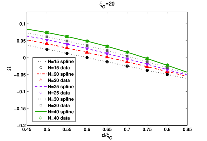
Figure 1: Plot of the subtracted $\Omega$ as a function of $\frac{d}{\xi_{G}}$ for $N=15,20,25,30,40$ and for the finest lattice, with $\xi_{G}=20$. The data point sizes are much larger than the statistical error bars which might be visible after significant magnification.

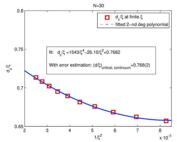
Figure 2: Extrapolation to continuum of $\frac{d_{c}(N)}{\xi_{G}}$ for N=30.

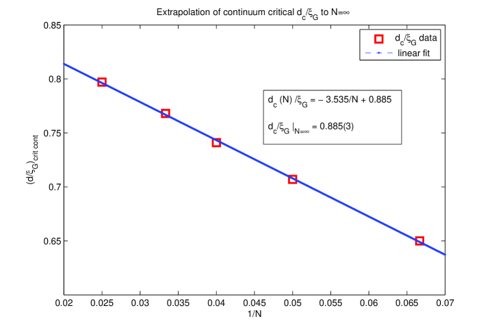
Figure 3: Extrapolation of $\frac{d_{c}(N)}{\xi_{G}}\left|{}_{\rm continuum}\right.$ to infinite $N$.

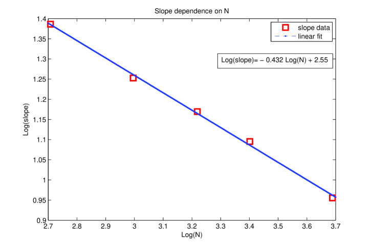
Figure 4: Testing for the critical exponent 1/2 in the slope variable.

For each $\xi_{G}$ in the range of 11 to 20 we end up with a $d_{c}(N)$ and a slope of $\Omega$ at $\Omega=0$. To check for a continuum limit we look at the ratios $\frac{d_{c}(N)}{\xi_{G}}$. For each value of $N$ we extrapolate to the continuum by fitting the data for $\frac{d_{c}(N)}{\xi_{G}}$ to a second order polynomial in $\frac{1}{\xi_{G}^{2}}$. This extrapolation is seen to be quite smooth and the second order polynomial provides a good fit. The slopes on the other hand have too low an accuracy to permit an extrapolation to the continuum limit; within their errors of a few percent they turn out to be $\xi_{G}$ independent. We took for the slopes the value on the finest lattice we have, at $\xi_{G}=20$ and carried out no continuum extrapolation.

Finally, we are ready to look at the $N$ dependence. For $d_{c}(N)$ we expect a convergence to an infinite $N$ linear in $\frac{1}{N}$. The slope of $d(N)$ with respect to $\Omega$ at $\Omega=0$ should go to zero as $\frac{1}{\sqrt{N}}$. Sample figures are below.

Figure 1 shows how the data for $\Omega$ is interpolated to get the critical size for a particular lattice spacing (the example is for $\xi_{G}=20$) at various values of $N$. Note that $\Omega$ gets steeper as $N$ increases. The data points markers are larger than the statistical jackknife errors.

Figure 2 shows the extrapolation to the continuum for $N=30$. The discrete value are plotted as squares to stand out, but the sizes of the squares do not indicate the errors. The error on the extrapolated value was computed by generating artificial noise on the input data with Gaussian errors of size determined by the jackknife estimates of the configuration averages. 40 such fake sets were next interpolated by cubic spline and then extrapolated to continuum to generate the error on the extrapolated value shown in the figure.

In Table 1 we summarize our findings. The definition of the entry “slope” is:

$$\left[\frac{d\left(d_{c}(N)/\xi_{G}\right)}{d\Omega}\right]_{\Omega=0}$$ (31)

$N$	$\left(\frac{d_{c}}{\xi_{G}}\right)_{continuum}$	slope
15	0.650(3)	-4.00
20	0.707(2)	-3.58
25	0.741(2)	-3.22
30	0.768(2)	-2.99
40	0.797(2)	-2.60

Table 1: Input to the extrapolation of $N$ to $\infty$

The final objective is to extrapolate to infinite $N$. For the critical size this is shown in Figure 3. We see that a simple linear extrapolation in $\frac{1}{N}$ works well and obtain in the infinite $N$ limit

$$\frac{d_{c}}{\xi_{G}}\left|{}_{continuum;~{}\tau=\frac{\xi_{G}^{2}}{300}}=0.885(3)\right.$$ (32)

Even if we accept that the $d_{c}(N)$ that we defined has a limit as described, we have presented so far little hard evidence that the transition is of the DO type. To see this, we look at the slope and check whether numerically it is plausible that it exhibits a dependence on $\sqrt{N}$ as the DO universality class would predict. In Figure 4 we show a plot of $\log|slope|$ versus $\log(N)$. One sees a slope that is different from the expected -0.5, but we have not included any further subleading corrections in $\frac{1}{N}$. There is little doubt that a slope of -1 is excluded by the data and the data is consistent with a slope of -0.5 in the asymptotic large $N$ regime. If we drop the lowest $N$ value from the fit the slope increases somewhat, but does not reach 0.5. The slopes for finite $N$ had too little accuracy to allow a continuum extrapolation and therefore we used only the slopes at $\xi_{G}=20$, our largest correlation length. There is no reasonable way to get a real error on our slope result, so no errors were quoted. Still, our result supports the expectation that the critical exponent associated with $d-d_{c}$ is 1/2.

Nothing we have done so far can be a substitute to a simple direct comparison of the DO eigenvalue distribution to the data. In Figure 5 and Figure 6 we show for N=40 plots of the eigenvalue density we obtained at $\xi_{G}=20$ for $d=10,21$ and $d=17$ respectively. Superposed on the data in both figures are the DO distributions obtained by fitting their single free parameter $k$. $k$ gives a measure for how far we are from the critical point which corresponds to $k_{c}=2$. Durhuus and Olesen obtained an expression for the distribution of the angle $\theta$ [4]. The eigenvalues of $W$ are $e^{\imath\theta_{j}}$, with $\sum_{j}\theta_{j}=0(mod)2\pi$ and $p(\theta)d\theta$ is the probability that any $\theta_{j}$ satisfy $|\theta_{j}-\theta|<d\theta/2$. $p(\theta)$ is defined from a complex function $h(k,\theta)$ which depends parametrically on $k$:

$$p(\theta)=-\frac{1}{2\pi k}{\rm Im\ }h(k,\theta).$$ (33)

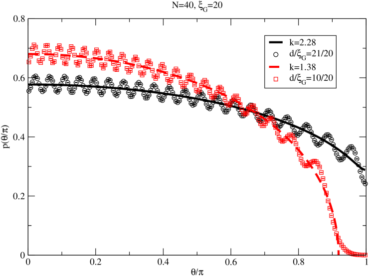
Figure 5: Examples of the eigenvalue distribution for a small ($d\sim 0.5\xi_{G}$) and a large distance ($d\sim\xi_{G}$).

The complex valued function $h(k,\theta)$ is determined by a nonlinear equation. One first introduces two $\theta$ dependent real variables, $x$ and $y$, and the expressions $f(y)=\frac{y}{\sinh(y)},~{}g(y)=y\coth(y)$.

$$x=-f(y)\sin(x+\theta),~{}~{}x+\theta={\rm Re\ }h(k,\theta),~{}~{}y={\rm Im\ }h(k,\theta)$$ (34)

These equations change variables from $h,\theta$ to $x,y,\theta$. The dependence on $k$ comes in through the main equation

$$g(y)-k=f(y)\cos(x+\theta)$$ (35)

$k$ determines the support of $p(\theta)$, which just reaches $\theta=\pm\pi$ at $k=k_{c}$.

$$|\theta|\leq\cases{\pi&if $k>2$\cr\cos^{-1}(1-k)+\sqrt{2k-k^{2}}&if $k<2$\cr}$$ (36)

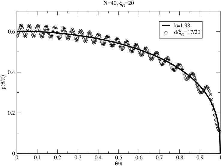
Figure 6: An example of an almost critical eigenvalue distribution ($d\sim 0.85\xi_{G}$).

In Figure 5 we see two extreme cases, one corresponding to a gapped eigenvalue distribution for a distance of the order $d=0.5\xi_{G}$ and the other for an eigenvalue distribution covering the entire unit circle, for a distance $d=1.05\xi_{G}$. The solid lines are the exact DO distribution, at a $k$ that was determined by the best least squares fit to the empirical histogram. Taking data for a larger set of distances then usual, we can ask which distance provides a $k$ closest to critical. It turns out that this happens at $d=17$, where $k=1.98$. Thus, this simple method would have given us an estimate for the infinite $N$ critical ratio $\frac{d_{c}}{\xi_{G}}$ of about $0.85$. Our result for our definition for a finite $N$ critical distance $d_{c}(N)$ for $N=40$ gave $\frac{d_{c}}{\xi_{G}}\sim 0.80$ at $\xi_{G}=20$ while the continuum infinite $N$ number was 0.885. This is all consistent. Figure 6 shows this close to critical distribution.

One may speculate that the DO distribution matches the continuum infinite $N$ distribution exactly in the critical case, but this is very likely not correct. Universality holds only for $\theta$ close to $\pm\pi$. If one looks at the integrated square distance between the DO distribution and the empirical one as a function of $N$ there is no evidence that this distance extrapolates to zero.

8 Summary.

There is little doubt that with the introduction of the smearing parameter $\tau$ the PCM undergoes an infinite $N$ phase transition of the DO type, in a manner analogous to smeared Wilson loops in two, three and four dimensions.

The PCM also offers the hope to establish this transition by analytic means. If this could be done, the role of the parameter $\tau$ could be further elucidated. We look at it as an extra renormalization of the two point matrix needed to reconcile its short distance behavior with it being a fluctuating unitary (and hence bounded) matrix.

At infinite $N$ the PCM model has a a trivial S-matrix for its set of bound states. Nevertheless, it is not a free field theory in terms of the variables $g(x)$ as evidenced by the short distance singularity of the two point function. The introduction of $\tau$ eliminates this divergence but since $\tau$ can be made very small, the short distance behavior of the two point function can be seen for $\sqrt{\tau}<<d<<\xi_{G}$. The DO transition occurs at $d\sim\xi_{G}$ and separates the two regimes, one of noninteracting bound states and the other of Gaussian fluctuations of the fundamental variable $g(x)$.

- [1] P. Rossi, M. Campostrini, E. Vicari, Phys. Rep. 302 (1998) 143.
- [2] R. Narayanan, H. Neuberger, JHEP 03 (2006) 064.
- [3] R. Narayanan, H. Neuberger, JHEP 0712 (2007) 066.
- [4] B. Durhuus and P. Olesen, Nucl. Phys. B 184, 461 (1981).
- [5] Y. Makeenko, “Methods of contemporary gauge theory”, Cambridge University Press, 2002.
- [6] R. A. Janik, W. Wieczorek, J. Phys. A: Math. Gen. 37, 6521 (2004).
- [7] D. V. Voiculescu, K. J. Dykema, A. Nica, “Free Random Variables” AMS — CRM, (1992).
- [8] P. Olesen, Nucl. Phys. B752 (2006) 197.
- [9] P. Olesen, Phys. Lett. B660 (2008) 597.
- [10] J-P Balizot, M. A. Nowak, arXiv:0801.1859 [hep-th].
- [11] P. Rossi, E. Vicari, Phys. Rev. D49 (1994) 1621.
- [12] R. Narayanan and H. Neuberger, Phys. Rev. Lett. 91, 081601 (2003) [arXiv:hep-lat/0303023].
- [13] J. Kiskis, R. Narayanan and H. Neuberger, Phys. Lett. B574 (2003) 65.