The Invertible Double of Elliptic Operators

Abstract.

First, we review the Dirac operator folklore about basic analytic and geometrical properties of operators of Dirac type on compact manifolds with smooth boundary and on closed partitioned manifolds and show how these properties depend on the construction of a canonical invertible double and are related to the concept of the Calderón projection. Then we summarize a recent construction of a canonical invertible double for general first order elliptic differential operators over smooth compact manifolds with boundary. We derive a natural formula for the Calderón projection which yields a generalization of the famous Cobordism Theorem. We provide a list of assumptions to obtain a continuous variation of the Calderón projection under smooth variation of the coefficients. That yields various new spectral flow theorems. Finally, we sketch a research program for confining, respectively closing, the last remaining gaps between the geometric Dirac operator type situation and the general linear elliptic case.

0. Introduction

This paper reviews our recent results, obtained jointly with Chaofeng Zhu [7], about basic analytical properties of elliptic operators on compact manifolds with smooth boundary. Furthermore, we outline a research program for confining, respectively closing, the last remaining gaps between the geometric Dirac operator type situation and the general linear elliptic case.

Our main results are

• to develop the basic elliptic analysis in full generality, and not only for the generic case of operators of Dirac type in product metrics (i.e., we assume neither constant coefficients in normal direction nor symmetry of the tangential operator);

• to give an analytical proof of the cobordism invariance of the index in greatest generality; and

• to prove the continuity of the Calderón projection and of related families of global elliptic boundary value problems under parameter variation.

Most analysis of geometrical and physical problems involving a Dirac operator $A$ on a compact manifold $M$ with smooth boundary $\partial M$ acting on sections of a (complex) bundle $E$ seems to rely on quite a few basic facts which are part of the shared folklore of people working in this field of global analysis. See, e.g., [10] for

• the weak inner unique continuation property (also called weak UCP to the boundary), i.e., there are no nontrivial elements in the null space $\ker(A)$ vanishing at the boundary of $M$;

• the existence of a suitable elliptic invertible continuation $\widetilde{A}$ of $A$, acting on sections of a vector bundle over the closed double or another suitable closed manifold $\widetilde{M}$ which contains $M$ as submanifold; this yields a Poisson type operator $K_{+}$ which maps sections over the boundary into sections in $\ker A$ over $M$; and a precise Calderón projection $C_{+}$ ;

• the existence of a self-adjoint regular Fredholm extension of any total (formally self-adjoint) Dirac operator $A$ in the underlying $L^{2}$-space with domain given by a pseudodifferential boundary condition; that actually is equivalent to the Cobordism Theorem asserting a canonical splitting of the tangential operator $B=B^{+}\oplus B^{-}$ with $\operatorname{ind}(B^{+})=0$;

and Nicolaescu [20, Appendix] and Booß, Lesch and Phillips [6] for

• the continuous dependence of a family of operators, their associated Calderón projections, and of any family of well-posed (elliptic) boundary value problems on continuous or smooth variation of the coefficients.

We will show that these results, with slight modifications, do hold for arbitrary first order elliptic operators.

We are fully aware that Dirac operators are attractive because they have an obvious geometrical meaning like the Laplace operator, probably the most important elliptic operator, for physicists as well as mathematicians. In the present paper we show that the above mentioned results for the Dirac operator do hold, with slight modifications, for arbitrary first order elliptic operators. As a matter of fact, the methods applied can be extended to general elliptic systems (of higher order) in a very natural way. However, in this paper we shall restrict ourselves to first order systems, mostly for the ease of presentation and the clarity of the essential constructions and proofs.

It is therefore not unreasonable to ask How special are operators of Dirac type compared to arbitrary linear first order elliptic differential operators? Our treatment of that question here may be used as a guide for addressing corresponding questions for general elliptic systems of higher order. Roughly speaking, our message is that the basic geometric aspects of geometrically defined operators like the Dirac operator (and the Laplace operator, when extending to higher order) have their root in the very ellipticity, i.e., in the symmetry properties of the principal symbol. The beautiful underlying metric properties leading to the definition of these operators make proofs of the basic geometric facts easier but are, as we shall show, dispensable.

We were led to our deformation question by a variety of mathematical and physical motivations. We mention

• the continuing interest in contact manifolds and CR-structures and the corresponding tangential CR-complexes (see, e.g., the classic monograph Boggess [4] or the recent Ponge [26]);

• stability questions in Electrical Impedance Tomography (see, e.g., the original problem in Calderón [14] and the recent Kenig and Sjöstrand [19], dealing, though, with the robustness of the Dirichlet-to-Neumann operator for elliptic second order equations instead of the Calderón projection for first order operators dealt with in this Note);

• deformations in Quantum Gravity which tear and/or burst classical field theories (see the visions disseminated, e.g., in Nielsen and Ninomiya [21]);

• but most of all our own curiosity about the extent to which simple geometric properties not only predetermine and guide analytic investigation but also pin down the results.

It has been known for half a century that, e.g., the K-groups of spin manifolds are generated by the index classes of Dirac operators up to torsion. For concrete calculations, however, many technical arguments depend on constructions which work only for geometrically defined operators of Dirac type and under the additional assumption that all metric structures are product near the boundary $\partial M$ of the underlying smooth compact Riemannian manifold $M$.

One of such technical devices is the invertible double, proved in Booß and Wojciechowski [10]. For the precise formulation and a sketch of proof see below Proposition 1.4.

For more general elliptic operators, as arising from first-order deformations, an invertible elliptic extension is often assumed “for convenience”. Actually, for Dirac type operators in the non–product case, one can still extend the collar a bit and deform to the product situation. The resulting operator will still be invertible; however it will neither be an exact double, nor will it be canonical.

Although a geometric invertible double is not available in general, in this Note we shall show that there is always a nice boundary value problem which provides an “invertible” double and that important properties, previously established rigorously only for Dirac type operators remain valid for general elliptic operators.

The paper ist organized as follows:

In Section 1, we summarize the Dirac operator folklore with emphasis on the product property, weak inner UCP, the precise invertible double, and a sketch of the geometric role of the Calderón projection. Some of the results are counter-intuitive in spite of their basic and fundamental character. E.g., the local solvability of elliptic equations is well-known from classical theory, but it remains a surprise that, e.g., the precise double of the Cauchy–Riemann operator (obtained by twisting the complex line bundle, see below) is well defined, has smooth coefficients and is invertible - without subtracting projections on original or arising kernels.

In Section 2, we present the first main result of this article, namely the construction of a precise invertible double for any first order elliptic differential operator, satisfying weak inner UCP, respectively, an invertible double after subtracting the projection onto the inner (ghost) solutions. The novelty of our approach lies in the canonical character of the construction - in difference to the ingenious ideas of Seeley [29], [31] of the late 1960s which also provided an invertible double, but involved extensions and choices which excluded to follow, e.g., the parameter dependence and neither yielded the Lagrangian property of the Cauchy data spaces in the case of symmetric coefficients.

In Section 3, we present the other main results of this article, namely various applications of our construction of the invertible double. Surprisingly, it turns out that the investigation of the mapping properties of the induced Poisson operators and Calderón projections is by no means straightforward. It may be worth recalling the decisive role of the socalled Atiyah–Patodi–Singer spectral projections of the induced symmetric tangential operator over the boundary in the Dirac operator case. In our general case, that nice tool must be replaced by sectorial projections. Nevertheless, we can in this Section 3 establish

• the Lagrangian property of the Cauchy data space for formally self-adjoint coefficients;

• a Cobordism Theorem for any elliptic operator bounding a first order elliptic differential operator; and

• a couple of theorems analyzing the dependence of the Calderón projection on the input data.

We emphasize that all these results are stated for general first order elliptic differential operators. It is neither assumed that the operator is of Dirac type nor is product structure near the boundary assumed.

The proofs are intricate. We only give sketches of the proofs and made full-length proofs available at arXiv, Booß, Lesch and Zhu [7].

Three years ago, before our results were achieved, the first author made a “poll” at a conference of experts in global analysis about the correctness of our at that time only conjectures: about one half of the people present at that meeting thought the claims were more or less clear and almost proved already in the late 60s or early 70s. The other half doubted the claims and would bet on counter-examples.

In Section 4, we explain why we do not consider the reached results for optimal; what difficulties must be overcome; and what ideas might turn out to be worth following. In particular, it seems to us that a much better understanding of the analysis and geometry of sectorial projections is mandatory for further work on the mapping properties; and that the time perhaps has come for new approaches towards UCP, namely by focusing on weak inner UCP.

1. Dirac operator folklore

1.1 Product property of operators of Dirac type.

Let $M$ be a smooth compact oriented Riemannian manifold of dimension $m$ (with or without boundary) and let $E\to M$ be a Hermitian vector bundle of Clifford modules with the Clifford multiplication ${\mathbf{c}}:\Gamma^{\infty}(M;TM\otimes E)\to\Gamma^{\infty}(M;E)$. We recall that any choice of a smooth connection (covariant derivative) $\nabla:\Gamma^{\infty}(M;E)\to\Gamma^{\infty}(M;T^{*}M\otimes E)$ defines a (total) operator of Dirac type $A:={\mathbf{c}}\circ\nabla:\Gamma^{\infty}(M;E)\longrightarrow\Gamma^{\infty}(M;E)$, acting on the space $\Gamma^{\infty}(M;E)$ of smooth sections under the Riemannian identification of the bundles $TM$ and $T^{\ast}M$.

In local coordinates we have

(1.1) $$A=\sum_{i,j=1}^{m}g^{ij}\mathbf{c}(\frac{\partial}{\partial x_{i}})\frac{\partial}{\partial x_{j}}+\text{ zero order terms}.$$

It follows at once that the principal symbol $\sigma_{1}(D)(p,\xi)$ is given by Clifford multiplication by $i\xi$, so that any operator of Dirac type is elliptic with symmetric principal symbol. Denoting by $A^{t}$ the formal adjoint of $A$ we have Green’s formula

(1.2) $$({A}s,s^{\prime})-(s,{A^{t}}s^{\prime})=-\int_{\partial M}\langle J(s|_{\partial M}),s^{\prime}|_{\partial M}\rangle,\quad s,s^{\prime}\in\Gamma^{\infty}(M;E).$$

Here $J:={\mathbf{c}}({\bf n}):E|_{\partial M}\to E|_{\partial M}$ denotes the unitary bundle isomorphism given by Clifford multiplication by the inward unit tangent vector with $J^{2}=-I$.

If the connection $\nabla$ is compatible with Clifford multiplication (i.e. $\nabla\mathbf{c}=0$) and unitary (i.e. Leibniz’ rule $X\langle s,s^{\prime}\rangle=\langle\nabla_{X}s,s^{\prime}\rangle+\langle s,\nabla_{X}s^{\prime}\rangle$ holds for $s,s^{\prime}\in\Gamma^{\infty}(M;E),X\in\Gamma^{\infty}(TM)$), then the operator $A$ itself becomes formally self–adjoint.

Let $\gamma_{5}$ denote the global section of $\operatorname{Hom}(E,E)$ defined locally by $\gamma_{5}:={\mathbf{c}}(e_{1})\dots\mathbf{c}(e_{m})$ (for a positively oriented orthonormal local frame). If $m$ is even, e.g., $m=4$ as in many physics applications, $E$ splits into subbundles $E^{\pm}$ . They are spanned by the eigensections of $\gamma_{5}$ corresponding to the eigenvalue $\pm 1$, if $m$ is divisible by 4, or $\pm i$ otherwise. The Clifford multiplication $J$ switches between $E^{\pm}|_{\partial M}$ and $E^{\mp}|_{\partial M}$. If $\nabla$ is compatible and unitary the Dirac operator splits correspondingly into components ${A}=\bigl{(}\begin{smallmatrix}0&A^{-}\\ {A}^{+}&0\end{smallmatrix}\bigr{)}$ such that the right chiral (half) Dirac operator ${A}^{+}:\Gamma^{\infty}(M;E^{+})\to\Gamma^{\infty}(M;E^{-})$ is formally adjoint to ${A}^{-}:\Gamma^{\infty}(M;E^{-})\to\Gamma^{\infty}(M;E^{+})$.

From (1.1) we derive a product property which distinguishes operators of Dirac type from general elliptic differential operators of first order.

Lemma 1.1.

Let $\Sigma$ be a closed hypersurface of $M$ with orientable normal bundle. Let $x$ denote a normal variable with fixed orientation such that a bicollar neighborhood ${N}$ of $\Sigma$ is parametrized by $[-\varepsilon,+\varepsilon]\times\Sigma$. Then any operator of Dirac type can be rewritten in the form

(1.3) $${A}|_{{N}}=\mathbf{c}(\frac{\partial}{\partial x})\left(\frac{\partial}{\partial x}+B_{x}+C_{x}\right),$$

where $B_{x}$ is a self-adjoint elliptic operator on the parallel hypersurface $\Sigma_{x}$, and $C_{x}:E|_{\Sigma_{x}}\rightarrow E|_{\Sigma_{x}}$ is a skew-adjoint operator of $0$th order, i.e., a skew-symmetric bundle homomorphism.

We shall call the operator $B_{0}+C_{0}$ the tangential component of $A$ in direction $\Sigma$. Its principal symbol is symmetric.

If the Riemannian metric of $M$, the Hermitian structure of $E$ and the connection $\nabla$ are product near the boundary, it follows from Lemma 1.1 (re-writing $B_{0}+C_{0}=:B$) that each operator of Dirac type takes the form

(1.4) $$A=J(\frac{d}{dx}+B)\quad\text{close to $\partial M$,}$$

with $J,B$ independent of the normal variable $x$ and $B$ a first order elliptic differential operator on $\partial M$. $B$ is not necessarily self–adjoint but has self–adjoint leading symbol. If the connection $\nabla$ is compatible and unitary then $A$ and $B$ are (formally) self–adjoint and this then implies $JB=-BJ$.

1.2 Unique Continuation Property (UCP) for operators of Dirac type.

Let $A$ be a linear or non–linear operator, acting on functions or sections of a bundle $E$ over a compact or non–compact connected manifold $M$.

(a) The operator $A$ has the strong UCP if any solution $u$ of the equation $Au=0$ has the following property: if $u$ vanishes at a point $p\in M$ with all its derivatives, then it vanishes on the whole of $M$.

(b) The operator $A$ has the weak UCP if any solution $u$ of the equation $Au=0$ has the following property: if $u$ vanishes on a nonempty open subset $\Omega$ of $M$, then it vanishes on the whole of $M$.

(c) Let $M$ be a compact manifold with boundary $\partial M$. Then the operator $A$ has the weak inner UCP (also called weak UCP “across the boundary”) if any solution $u$ of the equation $Au=0$ has the following property: if $u$ vanishes on $\partial M$, then it vanishes on the whole of $M$.

Let $A$ be an arbitrary elliptic differential operator $A$ of first order on a closed partitioned manifold $M=M_{-}\cup_{\Sigma}M_{+}$ , where $\Sigma$ is a hypersurface. Elliptic regularity and Green’s Formula imply (see, e.g., [10, Lemma 12.3]):

Lemma 1.2.

Any $u_{+}\in\Gamma^{\infty}(M_{+};E|_{M_{+}})$ with $Au_{+}=0$ and $u_{+}|_{\Sigma}=0$ can be continued to a smooth solution $u$ for the operator $A$ over the whole manifold $M$ by setting $u:=(u_{+},0)$.

The preceding Lemma implies that weak UCP  can be reformulated for linear elliptic differential operators of first order as UCP  across any hypersurface. More precisely, the operator $A$ has the weak UCP if any solution $u$ of the equation $Au=0$ has the following property: if $u$ vanishes on a hypersurface $\Sigma$, then it vanishes on the whole of $M$. In particular, weak UCP  implies weak inner UCP  for linear elliptic differential operators of first order.

Finally, by the same argument we see that weak UCP  implies UCP  across any single connected component of the boundary of $M$. More precisely, let $u$ be any solution of the equation $Au=0$ with $u|_{\Sigma_{1}}=0$ where $\Sigma_{1}$ is one connected component of the boundary $\Sigma$ of a compact connected manifold $M$. Then by weak UCP  it vanishes on all other components of $\Sigma$ and, in particular, it vanishes on the whole of $M$. Like so many other features of complex analysis, this tunneling property associated to weak UCP  is a bit counter–intuitive.

Weak UCP  is one of the basic properties of any operator of Dirac type. This can be seen by applying a hard result, obtained in 1956 independently by N. Aronszajn and H. O. Cordes for linear scalar elliptic operators of second order with smooth coefficients and with real principal symbol, to the Dirac Laplacian.

While the Aronszajn–Cordes Theorem yields strong UCP, there is also a direct proof on the level of the Dirac operator, exploiting Lemma 1.1, but yielding only weak UCP.

Theorem 1.3.

Let $M$ be a smooth compact connected Riemannian manifold and $A$ an elliptic differential operator of first order acting on sections in a Hermitian bundle. We assume that the tangential operator has symmetric principal symbol on every hypersurface $\Sigma$. Then $A$ satisfies weak UCP.

Sketch of proof.

Let $u$ be a solution of $Au=0$ which vanishes on an open nonempty set $\Omega$. We assume $\Omega=M\setminus\operatorname{supp}u$, i.e., maximal, namely the union of all open subsets on which $u$ vanishes.

First we localize and convexify the situation: since $M$ is connected, to prove that $\Omega=M$ it suffices to show that $\Omega$ is closed. So assume that $\partial\Omega=\overline{\Omega}\setminus\Omega$ is nonempty. Choose a $p\in\Omega$ whose distance from $\partial\Omega$ is less than the injectivity radius of $M$. Then we choose $p_{0}\in\partial\Omega$ with $\operatorname{dist}(p,p_{0})=\operatorname{dist}(p,\partial\Omega)$. In other words the open ball around $p$ with radius $r:=\operatorname{dist}(p_{0},p)$ is contained in $\Omega$, but $p_{0}\in\partial\Omega\subset\operatorname{supp}u$.

This construction provides us with a family of concentric hyperspheres $S_{p,x}$ of radius $x+r$. We fix an angular region by choosing $T>0$ with $T$ sufficiently small and inner radius $r$, ranging from the hypersphere $S_{p,0}$ which is contained in $\overline{\Omega}$, to the hypersphere $S_{p,T}$ which cuts deeply into $\operatorname{supp}u$, if $\operatorname{supp}u$ is not empty.

To conclude the localization, we replace the solution $u|_{\{S_{p,x}\}_{x\in[0,T]}}$ by a cutoff $v(x,y):=\phi(x)u(x,y)$ with a smooth bump function $\phi$.

Now we establish a Carleman inequality: for all $T>0$ sufficiently small and all $R>0$ sufficiently large we have

(1.5) $$\int_{0}^{T}\!\int_{S_{p,x}}\!\!e^{R(T-x)^{2}}\|v(x,y)\|^{2}dy\,dx\\ \leq\frac{2}{R}\int_{0}^{T}\!\int_{S_{p,x}}\!\!e^{R(T-x)^{2}}\|Av(x,y)\|^{2}dy\,dx,$$

for all arbitrary smooth sections $v$ (not necessarily a solution) with $\operatorname{supp}v\subset\{S_{p,x}\}_{x\in[0,T]}$ .

We apply (1.5) to our cutoff section $v(x,y)$ which by construction coincides with the solution $u$ for $x\leq 4/5T$ and vanishes identically for $x\geq 9/10T$. Elementary integral inequalities yield, that the solution $u$ must vanish in the whole annular region $0\leq x\leq T/2$ . This contradicts $p_{0}\in\operatorname{supp}u$, which proves the theorem. ∎

Details of the proof are given in [10, Chapter 8] and further elaborated, e.g., in Bleecker and Booß [3] and Booß, Marcolli and Wang [8]. Already Nirenberg [23, Sections 6–7, in particular the proof of his inequality (7.11)] pointed to the decisive role of the symmetry condition for deriving Carleman type inequalities.

1.3 The invertible double for operators of Dirac type.

After these preparations, we recall the invertible double construction from [10, Chapter 9].

Proposition 1.4.

Let $M$ be a smooth compact connected Riemannian manifold with boundary and let $A$ be a Dirac type operator on $M$ acting between sections of the Hermitian vector bundle $E$. Assume that all structures are product near the boundary. Then $A$ and $-A$ can be glued together to obtain an invertible elliptic operator $\tilde{A}=A\cup_{\partial M}(-A)$ on the closed double $\tilde{M}$.

Sketch of proof.

For simplicity we shall sketch the proof only for the total Dirac type operator and only in the formally self-adjoint case. The non-symmetric case and the chiral component operators require many, mostly notational modifications, see [10, Chapter 9].

Our starting point is the product form (1.4). The unitary map sending a section $f$ over $[0,\varepsilon)\times\partial M$ to $Jf(-.)$ over $(-\varepsilon,0]\times\partial M$ conjugates $A$ and $-A$. Hence if we use $J$ as a clutching function for the bundle $E$ then indeed $\tilde{A}=A\cup_{\partial M}(-A)$ is an elliptic operator with smooth coefficients on the double. Sections in $\operatorname{dom}(\tilde{A})$ can be viewed as pairs $(f_{+},f_{-})$, $f_{\pm}=f|_{M_{\pm}}$ such that $f_{-}|_{\partial M}=J(f_{+}|_{\partial M})$. Here $M_{\pm}$ denote the two different copies of $M$ in $\tilde{M}$.

To prove that $\widetilde{A}$ is invertible assume that $\tilde{A}f=0$. We then have $Af_{\pm}=0$. Green’s formula gives

$$\langle f_{\partial M},f_{\partial M}\rangle=\langle Af_{-},f_{+}\rangle-\langle f_{-},Af_{+}\rangle=0.$$

Thus $f|_{\partial M}=0$. The weak UCP  of Dirac operators (Theorem 1.3) then implies $f=0$. ∎

An illustration of the construction is given in [10, Chapter 26] in the simplest possible two–dimensional case, namely for the Cauchy–Riemann operator on the disc.

1.4 The geometric role of the Calderón projection.

The concept of an invertible double was used already 40 years ago to show that the Calderón projection $C_{+}$, i.e., the projection of $L^{2}(\partial M;E|_{\partial M})$ onto the space of Cauchy data $N_{+}^{0}:=\{u|_{\partial M}\in L^{2}(\partial M;E|_{\partial M})\mid Au=0\}$ is a pseudo–differential operator (Seeley [29], [31]) for any elliptic differential operator of first order. Various choices, however, entered into the original construction of the invertible double, while the preceding construction for Dirac type operators and product metrics close to the boundary is canonical. That provides a formula for $C_{+}$ in terms of $A$ such that the Lagrangian property $(N_{+}^{0})^{\perp}=JN_{+}^{0}$ is implied, see [10, Corollary 12.6], and mapping properties and dependencies on the data become transparent, see [6]. Only recently, the authors of this short review were able to prove similar results for general elliptic differential operators of first order, in collaboration with C. Zhu [7] (see Theorems 3.2, 3.4, and 3.5 below).

To give the reader the taste of the geometric meaning of $C_{+}$ we recall a few results for spectral invariants of Dirac type operators on manifolds with smooth boundary and on closed partitioned manifolds.

(A) The index of a well-posed boundary value problem $A^{+}_{P}$ for $A^{+}$ defined by a pseudo-differential projection $P$ with the same principal symbol as $C_{+}$ is given by the relative index of $P,C_{+}$, that is the index of the Fredholm operator $PC_{+}:\operatorname{im}C_{+}\to\operatorname{im}P$. On a closed partitioned manifold the index of a (chiral) Dirac operator $A^{+}$ can be identified with the index of the Fredholm pair of Cauchy data spaces along the partitioning hypersurface $\Sigma$.

For various extensions of this Bojarski Formula to the subelliptic case and for recent implications for the Atiyah-Weinstein conjecture see Epstein [15] and references given there.

An interesting feature of the Calderón projection for the Euclidean Dirac operator on the 4–ball is that it is $\gamma_{5}$ invariant, defines a self-adjoint boundary problem, and that the corresponding domain is gauge–invariant. As shown in Booß-Morchio-Strocchi-Wojciechowski [9], this property of the Calderón projection refutes the common claim of Quantum Chromodynamics according to which so-called naturality (i.e., gauge invariance of the domain and self-adjointness and $\gamma_{5}$ invariance of the boundary condition) implies chiral anomaly. The claim was suggested in Ninomiya and Tan [22]. It was based on a (here) misleading property of the Atiyah-Patodi-Singer boundary condition, namely the non-vanishing index of the chiral problem in general. Actually, this chiral anomaly would be an obstruction for zeta-function regularization of the determinant, as explained in [9]. Happily, the Calderón projection defines a boundary condition which gives vanishing index and, in fact, vanishing kernel and cokernel.

(B) The spectral flow of a curve of (total) Dirac operators with continuously varying connections over a closed partitioned manifold equals the Maslov index of the corresponding curves of Cauchy data spaces.

(C) The $\zeta$–determinant of a well-posed self-adjoint boundary value problem $A_{P}$ equals the Fredholm determinant of a canonically associated operator over the boundary up to a constant which can be identified with the $\zeta$–determinant of $A_{C_{+}}$ .

For proofs, we refer to [10] for (A), to Nicolaescu [20] for (B), and to Scott and Wojciechowski [28] for (C).

2. Invertible double for general first order elliptic operators

Let $M$ be a smooth compact connected Riemannian manifold with boundary and let $A:\Gamma^{\infty}(M;E)\longrightarrow\Gamma^{\infty}(M;F)$ be a first order elliptic differential operator acting between sections of the Hermitian vector bundles $E,F$. As above we separate variables in a collar $U$ of the boundary and write

(2.1) $$\begin{split}A|_{U}&=J_{0}\bigl{(}\frac{d}{dx}+B_{0}\bigr{)}+C_{1}x+C_{0},\\ A^{t}|_{U}&=\bigl{(}-\frac{d}{dx}+B_{0}^{t}\bigr{)}J_{0}^{*}+\widetilde{C}_{1}x+\widetilde{C}_{0},\end{split}$$

with bundle morphisms $J_{0},C_{0},\widetilde{C}_{0}$ ; $B_{0}$ a first order elliptic differential operator on $\partial M$; and $C_{1},\widetilde{C}_{1}$ first order differential operators on $U$. Put $\tilde{A}:=A\oplus(-A^{t})$, acting on sections of $E\oplus F$. $A^{t}$ denotes the formal adjoint of $A$. We choose a bundle morphism $T\in\operatorname{Hom}(E|_{\partial M},F|_{\partial M})$ and impose the boundary condition $({f_{+}},{f_{-}})\in\operatorname{dom}(\tilde{A}_{T}):\Leftrightarrow{f_{-}}|_{\partial M}=T{f_{+}}|_{\partial M}\Leftrightarrow({f_{+}}|_{\partial M},{f_{-}}|_{\partial M})\in\ker\begin{pmatrix}-T&\operatorname{Id}\end{pmatrix}.$

The two most important cases are $T:=(J_{0}^{*})^{-1}$ and, if $J_{0}=-J_{0}^{*}$, $T:=J_{0}|J_{0}|^{-1}$. In both cases the endomorphism $J_{0}^{*}T$ is positive definite.

Theorem 2.1.

Assume that $J_{0}^{*}T$ is positive definite. Then

1. $\tilde{A}_{T}$ is a realization of a local elliptic boundary condition (in the classical sense of Šapiro-Lopatinskiǐ), hence $\tilde{A}_{T}$ is a Fredholm operator with compact resolvent.

2. $\ker\tilde{A}_{T}=Z_{0}(A)\oplus Z_{0}(A^{t})\ \mbox{\ \rm and }\ \operatorname{coker}\tilde{A}_{T}\cong\ker\tilde{A}_{T}^{*}=Z_{0}(A^{t})\oplus Z_{0}(A)$.

Remark 2.2.

Here $Z_{0}(A)=\bigl{\{}u\in L^{2}(M,E)\,|\,Au=0,u|_{\partial M}=0\bigr{\}}$ denotes the space of “ghost solutions”. By elliptic regularity it is easy to see that $Z_{0}(A)$ is a finite–dimensional subspace of $\Gamma^{\infty}(M;E)$ and hence does not depend on the choice of a Sobolev regularity for $u$. $Z_{0}(A)=\{0\}$ if and only if weak inner UCP  holds for $A$. While weak UCP  can be proved for Dirac type operators in various ways (see above Section 1.4), it is generally believed that weak inner UCP does not hold for all first order elliptic differential operators, and it is open whether weak UCP  for $A$ implies weak UCP  for $A^{t}$, as conjectured by L. Schwartz [27], cf. below Section 4.2 for all that.

If the operator $A$ is formally self–adjoint, then for $T:=J_{0}|J_{0}|^{-1}$ the double $\tilde{A}_{T}$ is self–adjoint.

Sketch of proof of Theorem 2.1; for details cf. [7, pp. 6–12, 20–23].

As explained above the boundary condition for $\widetilde{A}_{T}$ is given by the bundle homomorphism $P(T)=\begin{pmatrix}-T&\operatorname{Id}\end{pmatrix}$.

From (2.1) we see that the tangential operator of $\widetilde{A}$ has leading symbol $b_{0}\oplus-(J_{0}^{t})^{-1}b_{0}^{*}J_{0}^{t}$, $b_{0}:=\sigma^{1}_{B(0)}$. Consequently the positive spectral projection of $b_{0}\oplus-(J_{0}^{t})^{-1}b_{0}^{*}J_{0}^{t}$ is given by $P_{+}(b_{0})\oplus(J_{0}^{t})^{-1}P_{-}(b_{0}^{*})J_{0}^{t}$. For an endomorphism $b$ of a finite–dimensional vector space $P_{\pm}(b)$ denotes the spectral projection corresponding to a closed contour encircling all eigenvalues $\lambda$ with $\operatorname{Re}\lambda\geq 0$ (respectively $<0$).

We recall from Hörmander [18, Definition 20.1.1] (see also [10, Remark 18.2d]) that $P(T)$ defines a local elliptic boundary condition for the operator $\widetilde{A}$ (or, equivalently, $P(T)$ satisfies the Šapiro-Lopatinskiǐ condition for $\widetilde{A}$), if and only if the principal symbol $\sigma^{0}_{P(T)}$ of $P(T)$ maps the positive spectral subspace of the leading symbol of the tangential operator, that is the space $\operatorname{im}P_{+}(b_{0}(y,\zeta))\oplus\operatorname{im}(J_{0}^{t})^{-1}P_{-}(b_{0}(y,\zeta)^{*})$, isomorphically onto the fibre $F_{y}$ for each point $y\in\Sigma$ and each cotangent vector $\zeta\in T^{*}_{y}(\Sigma)$, $\zeta\neq 0$. This statement is easily seen to be equivalent to the original definition, which refers to bounded solutions of an ode on the half line.

We now consider the Šapiro-Lopatinskiǐ mapping $\sigma^{0}_{P(T)}=(-T\,\operatorname{Id})$ from $\operatorname{im}P_{+}(b_{0}(y,\zeta))\oplus(J_{0}^{t})^{-1}\operatorname{im}P_{-}(b_{0}(y,\zeta)^{*})$ to $F_{y}$:

$$\bigl{(}e_{+},(J_{0}^{t})^{-1}e_{-}\bigr{)}\mapsto-Te_{+}+(J_{0}^{t})^{-1}e_{-}.$$

Multiplying by $J_{0}^{t}$ we see that this map is bijective if and only if the map $E_{y}=\operatorname{im}P_{+}(b_{0}(y,\zeta))\oplus\operatorname{im}P_{-}(b_{0}(y,\zeta)^{*})\longrightarrow E_{y},$

(2.2) $$(e_{+},e_{-})\mapsto-J_{0}^{t}Te_{+}+e_{-}$$

is bijective. Since the dimensions on the left and on the right coincide it suffices to show injectivity: so let $-J_{0}^{t}Te_{+}+e_{-}=0,$ $e_{+}\in\operatorname{im}P_{+}(b_{0}(y,\zeta)),$ $e_{-}\in\operatorname{im}P_{-}(b_{0}(y,\zeta)^{*})=\operatorname{im}P_{+}(b_{0}(y,\zeta))^{\perp}$. Taking scalar product with $e_{+}$ we find $0=-\langle J_{0}^{t}Te_{+},e_{+}\rangle$. This implies, since by assumption $J_{0}^{t}T>0$, that $e_{+}=0$. But then $e_{-}=0$ as well.

Thus it is proved that $P(T)$ satisfies the Šapiro-Lopatinskiǐ condition. This implies that $\widetilde{A}_{T}$ is a Fredholm operator with compact resolvent. In particular $\widetilde{A}_{T}$ has closed range and hence $\operatorname{coker}\tilde{A}_{T}\cong\ker\tilde{A}_{T}^{*}$.

If $f_{+}\in Z_{0}(A),f_{-}\in Z_{0}(A^{t})$ then $(f_{+},f_{-})=f\in\ker\tilde{A}_{T}$ since ${f_{-}}|_{\partial M}=0=T{f_{+}}|_{\partial M}$. Conversely, let $(f_{+},f_{-})=f\in\ker\tilde{A}_{T}$. Then certainly $f_{+}\in\ker A,f_{-}\in\ker A^{t}$ and ${f_{-}}|_{\partial M}=T{f_{+}}|_{\partial M}$. Since $J_{0}^{t}T$ is nonnegative and invertible, the operator $W:=(J_{0}^{t}T)^{{1/2}}$ exists and is invertible. Now Green’s formula (1.2) yields

(2.3) $$\begin{split}\|W{f_{+}}|_{\partial M}\|^{2}&=\langle{f_{+}}|_{\partial M},J_{0}^{t}T{f_{+}}|_{\partial M}\rangle=\langle J_{0}{f_{+}}|_{\partial M},{f_{-}}|_{\partial M}\rangle\\ &=-\langle Af_{+},f_{-}\rangle+\langle f_{+},A^{t}f_{-}\rangle=0,\end{split}$$

and since $W$ is invertible we find ${f_{+}}|_{\partial M}=0$ and ${f_{-}}|_{\partial M}=T{f_{+}}|_{\partial M}=0$; hence $f\in Z_{0}(A)\oplus Z_{0}(A^{t})$. ∎

3. Applications

3.1 The Calderón projection.

From Theorem 2.1 the Calderón projection may be constructed in the usual way. Let $r_{\pm}({f_{+}},{f_{-}}):=f_{\pm}$ and $\varrho_{\pm}({f_{+}},{f_{-}}):={f_{\pm}}|_{\partial M}$ and denote by $\varrho^{*}$ the $L^{2}$–dual of $\varrho_{+}$. It is well known that $\varrho_{\pm}$ maps the Sobolev space $L^{2}_{s}(M,\ldots)$ continuously into $L^{2}_{s-1/2}(\partial M,\ldots)$ for $s>1/2$ and consequently $\varrho^{*}$ maps $L^{2}_{s}(\partial M,\ldots)$ continuously into $L^{2}_{s-1/2}(M,\ldots)$ for $s<0$. These constraints on $s$ cause some technical difficulties.

For the domain of $A_{\max}$ the mapping properties of $\varrho$ can be slightly improved. Namely, for $s\geq 0$ the trace map extends by continuity to a bounded linear map

(3.1) $$\mathscr{D}(A_{\max,s})=\bigl{\{}u\in L^{2}_{s}(M,E)\,\bigm{|}\,Au\in L^{2}_{s}(M,F)\bigr{\}}\\ \longrightarrow L_{s-{1/2}}^{2}({\partial M},E|_{\partial M}),\quad s\geq 0,$$

here the domain $\mathscr{D}(A_{\max,s})$ is equipped with the graph norm of $A$ in $L^{2}_{s}(M,E)$.

Definition 3.1.

Let $\widetilde{A}_{T}^{-1}$ denote the pseudoinverse of the operator $\widetilde{A}_{T}$. That is on $\operatorname{im}\widetilde{A}_{T}$ it is the inverse of $\widetilde{A}_{T}|_{(\ker\widetilde{A}_{T})^{\perp}}$, on $(\operatorname{im}\widetilde{A}_{T})^{\perp}$ it is defined to be zero. Put

$$K_{\pm}:=\pm r_{\pm}\tilde{A}_{T}^{-1}\varrho^{*}J_{0},\quad C_{+}:=\varrho_{+}K_{+},\quad C_{-}:=T^{-1}\varrho_{-}K_{-}\,.$$

Theorem 3.2.

Under the assumptions of Theorem 2.1 and under the additional technical assumption that the commutator $[B_{0}^{t},J_{0}^{*}T]$ is of order $0$ we have:

1. For $s\geq-1/2$ the operator $K_{+}$ maps $L_{s}^{2}(\partial M,E|_{\partial M})$ continuously into $L^{2}_{s+1/2}(M,E)\cap\ker A$.

2. $C_{\pm}$ are complementary idempotents with $\operatorname{im}{C_{+}}=N_{+}^{0}$ and $\operatorname{im}{C_{-}}=T^{-1}N_{-}^{0}$, $N_{-}^{0}$ being the Cauchy data space of $A^{t}$. If $T=(J_{0}^{*})^{-1}$ then $C_{\pm}$ are orthogonal projections.

Remark 3.3.

$[J_{0}^{t}T,B_{0}^{t}]=0$ for the choice $T=(J_{0}^{t})^{-1}$.

If $A=A^{t}$ and $B_{0}-B_{0}^{t}$ is of order $0$ then $[J_{0}^{t}T,B_{0}^{t}]$ is of order $0$ for $T\in\bigl{\{}(J_{0}^{*})^{-1},{J_{0}},{J_{0}}|J_{0}|^{-1}\bigr{\}}$.

Sketch of proof; for details cf. [7, pp. 12–20, 23–30].

The method is more interesting than this result, which looks pretty similar to what one gets from geometric invertible double constructions respectively invertible non–canonical closed extensions.

There is one tricky point, however, in 1. Namely the constraint on $s$ dictated by the Trace Theorem for Sobolev spaces, as explained above. From this the claim in 1. can easily be deduced only for $-1/2\leq s<0$.

To extend it to $s\geq 0$ (including the interesting case $s=0$) one could invoke the general theory of elliptic boundary value problems (e.g. Grubb [16]).

We prefer a more elementary approach which is also better suited to deal with parameter–dependence, see Subsection 3.3 below.

A crucial observation is that the tangential operator $B_{0}$ is not an arbitrary elliptic operator. Rather the ellipticity of $A$ implies that $B_{0}-it,t\in\mathbb{R},$ is elliptic in the parametric sense. This is much stronger than ellipticity (cf. Shubin [33] for definition and basic properties).

This observation allows us to introduce the operators

(3.2) $$Q_{+}(x) :=\frac{1}{2\pi i}\int_{\Gamma_{+}}e^{-x\lambda}(\lambda-B)^{-1}\,d\lambda\,,\qquad x>0,$$

(3.3) $$Q_{-}(x) :=\frac{1}{2\pi i}\int_{\Gamma_{-}}e^{-x\lambda}(\lambda-B)^{-1}\,d\lambda,\qquad x<0.$$

Here $\Gamma_{+}$ is a contour which encircles the eigenvalues of $B_{0}$ in the right half plane and such that $\operatorname{Re}z_{n}\to\infty$ if $z_{n}$ is on $\Gamma_{+}$ with $|z_{n}|\to\infty$; the contour $\Gamma_{-}$ in the left half plane encircles the complementary set of eigenvalues, see Figure 1.

         

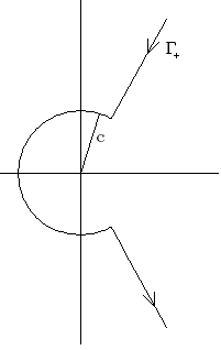
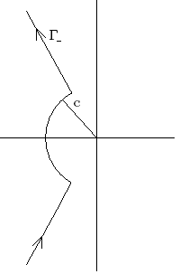
Figure 1. The contours $\Gamma_{\pm}$ in the plane defining the sectorial projections $Q_{\pm}$

It can be shown (cf. [7, Sec. 3.2]) that $P_{\pm}(B)=Q_{\pm}(0)$ is an a priory unbounded idempotent. It follows, however, from the work of Seeley [30], Burak [13], Wojciechowski [34], see also Ponge [25], that $P_{\pm}(B)$ is a pseudodifferential operator of order $0$. Intuitively, the positive/negative sectorial projections $P_{\pm}$ should map onto the subspaces spanned by the generalized eigenvectors corresponding to the eigenvalues encircled by the contours $\Gamma_{\pm}$. See, however, Remark 4.5 below.

The following approximation to $K_{+}$ constructed from $Q_{+}$ allows to control the error when replacing $C_{+}$ by the sectorial projection of $B_{0}$.

By direct calculation one checks ([7, Prop. 3.16], cf. also Himpel, Kirk and Lesch [17, Prop. 3.13] where the Spectral Theorem is used in the case of a symmetric tangential operator) that for $s\in\mathbb{R}$, a cut–off function $\varphi\in C^{\infty}_{0}(\mathbb{R}_{+})$ and $m\in\mathbb{Z}_{+}$ the operator

(3.4) $$\operatorname{id}_{\mathbb{R}_{+}}^{m}\varphi Q_{+}:\xi\mapsto\bigl{(}x\mapsto x^{m}\/\varphi(x)\/Q_{+}(x)\xi\bigr{)}$$

maps $L^{2}_{s}({\partial M},E|_{\partial M})$ continuously to $L^{2}_{\operatorname{comp}}(\mathbb{R}_{+},L^{2}_{s+m+{1/2}}({\partial M},E|_{\partial M}))$. Furthermore, for $s\geq-{1/2}$ it maps continuously to
$L^{2}_{s+m+{1/2},\operatorname{comp}}(\mathbb{R}_{+}\times{\partial M},E|_{{\partial M}})$. Put

(3.5) $$(R\xi)(x):=\begin{pmatrix}Q_{+}(x)\xi\\ Q_{-}(-x)^{*}\xi\end{pmatrix},\quad R_{T}\xi:=\begin{pmatrix}\operatorname{Id}&0\\ 0&-T\end{pmatrix}R\xi.$$

One checks the identity

(3.6) $$\widetilde{A}_{T}\varphi R_{T}\xi=\bigl{(}\varrho^{*}J_{0}(P_{+}+P_{-}^{*})+S(A,T)\bigr{)}\xi.$$

Beware that $\varphi R_{T}$ does not map into $\operatorname{dom}\widetilde{A}_{T}$. Therefore (3.6) has to be taken with a grain of salt. It is an identity in the “Sobolev space” $H_{-1}((\widetilde{A}_{T})^{*})$ which is the dual space of $\operatorname{dom}(\widetilde{A}_{T})$, where the latter is equipped with the graph norm. This fact is reflected in the appearance of $\varrho^{*}$. If one applies just the differential expression $\tilde{A}$ to $\varphi R_{T}\xi$ in $M\setminus{\partial M}$ then one obtains, by definition, $S(A,T)\xi$.

The reader should be warned that from the equality (3.6) one should not draw false conclusions about the mapping properties of $\varrho^{*}$. $\varphi R_{T}$ maps $L^{2}$ to $L^{2}_{1/2}$ but not to $H_{{1/2}}(\widetilde{A}_{T})$. So one cannot conclude (and it is indeed not true in general) that the right hand side of (3.6) lies in $H_{-{1/2}}(\widetilde{A}_{T})$. Nevertheless with some care one can derive the following identity from (3.6)

(3.7) $$\widetilde{A}_{T}^{-1}\varrho^{*}=\Bigl{(}(\operatorname{Id}-P_{Z_{0}(A)})\varphi R_{T}-\widetilde{A}_{T}^{-1}S(A,T)\Bigr{)}(J_{0}(P_{+}+P_{-}^{*}))^{-1}.$$

This identity yields the approximation $\varphi R_{T}((P_{+}+P_{-})^{*})^{-1}$ to $K_{+}$ near the boundary mentioned above. The mapping properties of $K_{+}$ can now be derived from those of $\varphi R_{T}$ and those of $S(A,T)$.

The mapping properties of $\varphi R_{T}$ were already quoted above. To calculate $\widetilde{A}\varphi R_{T}$ we proceed by component:

(3.8) $$A\varphi Q_{+}(x)\xi=\Bigl{(}(C_{1}x+C_{0})\varphi(x)+J_{0}\varphi^{\prime}(x)\Bigr{)}Q_{+}(x)\xi$$

and

(3.9) $$\begin{split}A^{t}\varphi TQ_{-}(-x)^{*}\xi&=\Bigl{(}(\widetilde{C}_{1}xT+\widetilde{C}_{0}T+[B_{0}^{t},J_{0}^{t}T])\varphi(x)-\ldots\\ &\quad-J_{0}^{t}\varphi^{\prime}(x)\Bigr{)}Q_{-}(-x)^{*}\xi.\end{split}$$

An immediate consequence of (3.8), (3.9) and (3.4) is that $S(A,T)$ maps $L^{2}_{s}({\partial M},E_{{\partial M}})$ continuously to $L^{2}_{s+{1/2},\operatorname{comp}}(M,F\oplus E)$, $s\geq-{1/2}$.

This establishes the regularity part of the claim. That $K_{+}$ maps indeed into $\ker A$ follows easily from the fact that $\varrho^{*}\xi$ is supported on ${\partial M}$ for any $\xi\in L^{2}_{s}({\partial M},...)$.

Since $K_{+}$ maps into $\ker A$ we have $C_{+}(L^{2})\subset N_{+}^{0},C_{-}(L^{2})\subset T^{-1}N_{-}^{0}$. We show

(i) $N_{+}^{0}\cap T^{-1}N_{-}^{0}=\{0\}$,

(ii) $C_{+}\,+\,C_{-}=\operatorname{Id}$.

This easily implies part 2. of the Theorem.

(i) Let $\xi\in N_{+}^{0}\cap T^{-1}N_{-}^{0}$. Then there are $f\in\ker A\cap L^{2}_{1/2}(M,E),g\in\ker A\cap L^{2}_{1/2}(M,F)$ with $\varrho f=\xi=T^{-1}\varrho g$. Then

(3.10) $$(f,g)\in\ker\widetilde{A}_{T}=Z_{0}(A)\oplus Z_{0}(A^{t}),\quad\text{by Theorem \ref{t:invdoub}.}$$

Since elements of $Z_{0}(A)\oplus Z_{0}(A^{t})$ vanish on the boundary we infer $\xi=0$.

(ii) Let $\xi\in L^{2}({\partial M},E|_{\partial M})$, and $f\in\operatorname{dom}(\widetilde{A}_{T}^{*})$. Then $\varrho_{+}f=-T\varrho_{-}f$ and exploiting the self–adjointness of $J_{0}^{t}T$ we obtain

(3.11) $$\begin{split}\langle(C_{+}&+C_{-})\xi,J_{0}^{t}\varrho_{+}f\rangle=\langle\varrho_{+}\widetilde{A}_{T}^{-1}\varrho^{*}J_{0}\xi-T^{-1}\varrho_{-}\widetilde{A}_{T}^{-1}\varrho^{*}J_{0}\xi,J_{0}^{t}\varrho_{+}f\rangle\\ &=\langle\varrho_{+}\widetilde{A}_{T}^{-1}\varrho^{*}J_{0}\xi,J_{0}^{t}\varrho_{+}f\rangle-\langle\varrho_{-}\widetilde{A}_{T}^{-1}\varrho^{*}J_{0}\xi,J_{0}J_{0}^{-1}(T^{-1})^{t}J_{0}^{t}\varrho_{+}f\rangle\\ &=\langle(\varrho_{+}\oplus\varrho_{-})\widetilde{A}_{T}^{-1}\varrho^{*}J_{0}\xi,(J_{0}^{t}\oplus J_{0})(\varrho_{+}f\oplus\varrho_{-}f)\rangle\\ &=\langle\widetilde{A}_{T}^{-1}\varrho^{*}J_{0}\xi,\widetilde{A}^{*}_{T}f\rangle=\langle\varrho^{*}J_{0}\xi,f\rangle=\langle\xi,J_{0}^{t}\varrho f\rangle.\end{split}$$

This proves (ii).

For $T=(J_{0}^{t})^{-1}$ one easily shows using Green’s formula that $N_{+}^{0}\perp T^{-1}N_{-}^{0}$, proving that $C_{\pm}$ are orthogonal projections in this case.

∎

3.2 A general Cobordism Theorem.

We shall now give a wide generalization of the Cobordism Theorem, previously known only for operators of Dirac type.

Theorem 3.4 (The General Cobordism Theorem).

Let $A$ be a first order formally self–adjoint elliptic differential operator on a smooth compact manifold $M$ with boundary acting between sections of the vector bundle $E$. Then we have the following results:

(I) Let $C_{\pm}$ denote the Calderón projections of Definition 3.1, constructed from the invertible double with ${T}\in\bigl{\{}(J_{0}^{*})^{-1},{J_{0}},{J_{0}}|J_{0}|^{-1}\bigr{\}}$. Then the range of $C_{+}$ is a Lagrangian subspace of the strongly symplectic Hilbert space $\bigl{(}L^{2}(\partial M,E|_{\partial M}),-{J_{0}}\bigr{)}$. Note that $\operatorname{im}C_{+}$ is independent of ${T}$. Consequently, there exists a self-adjoint pseudodifferential Fredholm extension $A_{P}$.

(II) We have $\operatorname{sign}iP_{0}{J_{0}}|_{W_{0}}=0$. Here $W_{0}$ denotes the (finite–dimensional) sum of the generalized eigenspaces of ${B_{0}}$ to imaginary eigenvalues and $P_{0}$ denotes the orthogonal projection onto $W_{0}$; in general ${J_{0}}$ will not map $W_{0}$ into itself. If ${B_{0}}={B_{0}}^{t}$ , then ${J_{0}}$ anticommutes with ${B_{0}}$ and we have $\operatorname{sign}i{J_{0}}|_{\ker{B_{0}}}=0$ and the tangential operator ${B_{0}}$ is odd with respect to the grading given by the unitary operator $\alpha:=i{J_{0}}(-{J_{0}}^{2})^{-1/2}$ and hence splits into matrix form ${B_{0}}=\bigl{(}\begin{smallmatrix}0&B^{-}\\ B^{+}&0\end{smallmatrix}\bigr{)}$ with respect to the $\pm 1$–eigenspaces of $\alpha$. The index of $B^{+}:\ker(\alpha-1)\longrightarrow\ker(\alpha+1)$ vanishes.

Sketch of proof; for details cf. [7, pp. 30–41].

The first claim, expressed in the language of symplectic functional analysis, follows immediately from our construction of the Calderón projection: Clearly $(u,v)\mapsto\langle-{J_{0}}u,v\rangle$ is a (strong) symplectic form for the Hilbert space $L^{2}(\partial M,E|_{\partial M})$. Then the range $\operatorname{im}(C_{+})=N_{+}^{0}$ is an isotropic subspace because of Green’s formula (1.2). It remains valid for arbitrary formally self-adjoint elliptic operators of first order and is here applied to $\ker A$. Here we use the symplectic $T:={J_{0}}|J_{0}|^{-1}$ to construct $C_{\pm}$ . That choice of $T$ yields a self-adjoint double $\tilde{A}_{T}$ as observed above. Then also $\operatorname{im}(C_{-})=T^{-1}(N_{+}^{0})$ is an isotropic subspace. By Theorem 3.2.2, we have $C_{+}+C_{-}=\operatorname{Id}$, so $N_{+}^{0}$ and $T^{-1}(N_{+}^{0})$ make a pair of transversal isotropic subspaces of $L^{2}(\partial M,E|_{\partial M})$. Then (I) follows from the simple algebraic observation, that transversal isotropic subspaces in a symplectic vector space must be Lagrangian (taken from Booß and Zhu [11, Lemma 1.2]).

To derive the second claim we split $L^{2}(\partial M,E|_{\partial M})$ into the spectral subspaces $W_{<}\,,W_{0}\,,W_{>}$ of $B_{0}$ corresponding to eigenvalues with negative, respectively zero, respectively positive real parts. The projections onto $W_{<},W_{>}$ are in fact versions of the positive/negative sectorial projections which are defined via contour integrals, cf. the proof of Theorem 3.2.

Then $(\operatorname{im}C_{+},W_{<})$ is a Fredholm pair by finite–dimensional perturbation. Hence $\operatorname{im}C_{+}\oplus W_{<}$ is a closed subspace.

We notice that the annihilator $W_{<}^{o}=W_{0}\oplus W_{<}$ is a co-isotropic subspace of $L^{2}(\partial M,E|_{\partial M})$. We apply symplectic reduction to the Lagrangian subspace $\operatorname{im}C_{+}$ and obtain that $\bigl{(}(\operatorname{im}C_{+})+W_{<}^{oo})\cap W_{<}^{o}\bigr{)}/W_{<}^{oo}$ is a Lagrangian subspace of $W_{<}^{o}/W_{<}^{oo}=(W_{<}+W_{0})/W_{<}\simeq W_{0}.$ So, the finite–dimensional symplectic Hilbert space $\bigl{(}W_{0},\langle iP_{0}{J_{0}}\cdot,\cdot\rangle\bigr{)}$ has a Lagrangian subspace. Therefore $\operatorname{sign}iP_{0}{J_{0}}|_{W_{0}}=0$. The remainder of (II) follows like in [10, Theorem 21.5]. ∎

3.3 Parameter dependence.

To study continuous variations, we equip the space $\mathscr{E}(M;E,F)$ consisting of pairs $(A,T)$ with $J_{0}^{*}T>0$ and $[B_{0}^{t},J_{0}^{*}T]$ of order 0 with the metric $d_{0}((A,T),(A^{\prime},T^{\prime}))$ := $N_{0}(A-A^{\prime},T-T^{\prime})$ and the strong metric $d_{\operatorname{str}}((A,T),(A^{\prime},T^{\prime})):=N_{0}(A-A^{\prime},T-T^{\prime})+N_{1}(A-A^{\prime},T-T^{\prime})$, where

$$N_{0}(A,T) :=\|A\|_{1,0}+\|A^{t}\|_{1,0}+\|T\|_{{1/2},{1/2}}\quad\mbox{\ \rm and }$$

$$N_{1}(A,T) :=\|B_{0}\|_{1,0}+\|B_{0}^{t}\|_{1,0}+\|[B_{0}^{t},J_{0}^{*}T]\|_{0}+\|T\|_{0}$$

$$\quad+\|J_{0}\|_{0}+\|C_{1}\|_{1,0}+\|C_{0}\|_{0}+\|\widetilde{C}_{1}\|_{1,0}+\|\widetilde{C}_{0}\|_{0}\,.$$

Here $\|\cdot\|_{s,t}$ denotes the norm for bounded operators from the Sobolev space $L^{2}_{s}(...)$ into the Sobolev space $L^{2}_{t}(...)$.

We denote by $\mathscr{E}_{\operatorname{UCP}}(M;E,F)$ the subspace consisting of pairs $(A,T)$ where $A$ and $A^{t}$ satisfy weak inner UCP and by $\mathscr{E}_{\operatorname{UCP}}^{\textup{sa}}(M;E,F)$ the subspace where $A$ has tangential operator with self–adjoint principal symbol. We denote by $\operatorname{Ell}^{\textup{sa}}_{\operatorname{UCP}}(M;E)$ the component of $\mathscr{E}^{\textup{sa}}_{\operatorname{UCP}}$ of formally self–adjoint operators, equipped with the strong metric.

Theorem 3.5.

(I) The map

$$(\mathscr{E}_{\operatorname{UCP}},d_{0})\longrightarrow\mathscr{B}(L^{2}(M,F\oplus E),L^{2}_{1}(M,E\oplus F)),\quad(A,T)\mapsto\tilde{A}_{T}^{-1}$$

is continuous.

(II) For $s\in[-{1/2},{1/2}]$ the map

$$(\mathscr{E}^{\textup{sa}}_{\operatorname{UCP}}(M;E),d_{\textrm{str}})\longrightarrow\mathscr{B}(L^{2}_{s}(\partial M,E|_{\partial M})),\quad(A,T)\mapsto C_{+}(A,T)$$

is continuous.

(III) The map $\operatorname{Ell}^{\textup{sa}}_{\operatorname{UCP}}(M;E)\longrightarrow\mathscr{B}(L^{2}_{1}(M,E),L^{2}(M,E))$, $A\mapsto A_{C_{+}}$ is continuous. Here $C_{+}$ denotes the version of the Calderón projection constructed from $T:=(J_{0}^{*})^{-1}$.

Sketch of proof; for details cf. [7, pp. 42–51].

To (I): The difficulty we are facing here is that $\operatorname{dom}\bigl{(}\widetilde{A}_{T}\bigr{)}$ varies with $T$. So we fix a $T_{0}$ close to $T$ and make the following factorization

(3.12) $$(A,T)\mapsto\tilde{A}_{T}\circ\Phi_{T_{0},T}\mapsto\bigl{(}\tilde{A}_{T}\circ\Phi_{T_{0},T}|_{\operatorname{dom}(\tilde{A}_{T_{0}})}\bigr{)}^{-1}\mapsto\tilde{A}_{T}^{-1}\,.$$

Here we set

$$\Phi_{T_{0},T}\binom{f_{+}}{f_{-}}:=\binom{f_{+}}{f_{-}+e(T-T_{0})\varrho f_{+}},$$

where $e$ denotes a linear right-inverse to $\varrho$ (as, e.g., in [10, Definition 11.7e]). The operator $\Phi_{T_{0},T}$ is bounded invertible on $L^{2}_{1}(M,E\oplus F)$ and maps $\operatorname{dom}\tilde{A}_{T_{0}}$ bijectively onto $\operatorname{dom}\tilde{A}_{T}$. Note that $\tilde{A}_{T}^{-1}=\Phi_{T_{0},T}\circ\bigl{(}\tilde{A}_{T}\circ\Phi_{T_{0},T}|_{\operatorname{dom}(\tilde{A}_{T_{0}})}\bigr{)}^{-1}$ . It is straightforward to check the continuity of the first and last arrow in (3.12), while the middle arrow is just the general continuous inversion for bounded operators in Banach space.

To (II): From (3.6) and (3.7) we obtain the correction formula

(3.13) $$C_{+}=\bigl{(}P_{+}-\varrho_{+}\tilde{A}_{T}^{-1}S(A,T)\bigr{)}(P_{+}+P_{-}^{*})^{-1}\,,$$

relating $C_{+}(A,T)$ and the sectorial projection $P_{+}:=P_{+}(B_{0})$ of the tangential operator $B(0)$. Note that (3.13) is valid for arbitrary $A$. Continuous variation of $\tilde{A}_{T}^{-1}$ and $S(A,T)$ can be obtained without restriction regarding $B_{0}$ in the same way as in the proof of (I). Continuous variation of $P_{+}$ can also be obtained for general $A$ and general $B_{0}$ if the variation is of order $<1$ [7, Prop. 7.13]. However, admitting variation of $A$ and $B_{0}$ of order 1, we obtain continuous variation of $P_{+}$ only for formally self-adjoint $B_{0}$ via a Riesz-map argument, see the discussion around Prop. 4.3 below.

To (III): Note that $A_{C_{+}}$ is self–adjoint by Theorem 3.4.II. It is indeed a self–adjoint realization of a well–posed boundary value problem. Applying the preceding (II) and a generalization of the preceding (I) (as indicated below in the Note to (I)) yields the claim. ∎

Remark 3.6.

(I) is much stronger than just graph continuity. In the same way, we obtain that the map

$$(A,P)\mapsto(A_{P}+i)^{-1}\in\mathscr{B}(L^{2}(M;E),L^{2}_{1}(M;E))$$

is continuous with respect to the $d_{0}$ metric on the space of pairs $(A,P)$ where $P$ is a pseudodifferential orthogonal projection which is well–posed with respect to $A$. In particular $(A,P)\mapsto(A_{P}+i)^{-1}$ is graph continuous.

The continuous dependence of the Calderón projection on the input data in (II) has consequences for the so–called Spectral Flow Theorem, cf. [11] and Section 1.4.B above.

In (III) we obtain a more precise version of [6], Theorem 3.9 (c). Note that our present version applies to a much wider class of operators than loc. cit.

For deformations of $A$ by a $0$th order operator the continuous variation of the Calderón projector was proved in a purely functional analytic context by Booß–Bavnbek and Furutani [5].

4. Closing, respectively confining, the gaps

4.1 Full elucidation of parameter dependence.

Dirac type operators and their Calderón projection vary continuously under variation of the underlying connection. Note that such variations are only perturbations by bounded operators. However, it is a disturbing gap in our perception of fundamental concepts of quantum field theory that we can not exclude the possibility that more general but still smooth variations of the coefficients can yield jumps of the Calderón projection when leaving the realm of Dirac type operators, even in the presence of a spectral cut.

In particular, for spectral flow formulas (see Subsection 1.4.B), the continuous dependence of the Calderón projection on the input data is crucial. In Section 3 we could establish this continuous dependence under the assumption that the tangential operator has self-adjoint leading symbol. We would like to get rid of this technical assumption. For this it is necessary to study the positive sectorial projection of a (non-self-adjoint) elliptic differential operator and its dependence on the input data.

In [7, Theorem 7.2] we in fact proved the following variant of Theorem 3.5 (II) for $(\mathscr{E}_{\operatorname{UCP}}(M;E),d_{\textrm{str}})$ instead of $(\mathscr{E}^{\textup{sa}}_{\operatorname{UCP}}(M;E),d_{\textrm{str}})$:

If $(A(z),T(z))$ is a continuous family in $(\mathscr{E}_{\operatorname{UCP}}(M;E),d_{\textrm{str}})$ such that the corresponding family of positive sectorial projections of the tangential operator varies continuously in $\mathscr{B}(L^{2}_{s}(\partial M,E|_{\partial M}))$ then $C_{+}(A(z),T(z))\in\mathscr{B}(L^{2}_{s}(\partial M,E|_{\partial M}))$ depends continuously on $z$, too.

So the continuous dependence of the Calderón projection in general hinges on the continuity of the positive sectorial projection of the tangential operator.

We can now phrase the problem completely in terms of a single elliptic operator on the closed manifold $\partial M$: fix contours $\Gamma_{+},\Gamma_{-}$ as in Figure 1 and denote by $\operatorname{Ell}^{1}_{\Gamma}(\partial M,E|_{\partial M})$ the space those differential operators $B$ on $\partial M$ acting on sections of the vector bundle $E|_{\partial M}$ such that firstly $B$ is elliptic and all eigenvalues of the leading symbol $\sigma^{1}_{B}(p,\xi)$ are encircled by $\Gamma_{+}\cup\Gamma_{-}$ and secondly no eigenvalue of $B$ lies on the curves $\Gamma_{\pm}$.

The first condition means in other words that for $\xi\in T_{p}^{*}M\setminus\{0\}$ there are no eigenvalues of the leading symbol of $B$ inside the sectors around the imaginary axis with boundary defined by the legs of $\Gamma_{\pm}$.

Note that a self–adjoint operator is in $\operatorname{Ell}^{1}_{\Gamma}(\partial M,E|_{\partial M})$ if and only if $\pm c\not\in\operatorname{spec}B$.

For $B\in\operatorname{Ell}_{\Gamma}^{1}(\partial M,E|_{\partial M})$ the operator families $Q_{\pm}$, in particular the positive sectorial projections $P_{\pm}$, as defined in the proof of Theorem 3.2, are available.

Now we can formulate the main problem related to the continuous variation of the Calderón projection:

Problem 4.1.

For which (reasonable) topology on $\operatorname{Ell}_{\Gamma}^{1}(\partial M,E|_{\partial M})$ is the map

(4.1) $$\operatorname{Ell}_{\Gamma}^{1}(\partial M,E|_{\partial M})\longrightarrow\mathscr{B}(L^{2}(\partial M,E|_{\partial M}),\quad B\mapsto P_{\pm}(B)$$

continuous?

For our original operator $A$ with tangential operator $B_{0}$ (cf. (2.1)) we only have a reasonable chance for $P_{\pm}(B_{0})$ to depend continuously on $A$ if $B_{0}$ depends continuously on $A$, too. So the next problem is

Problem 4.2.

Suppose the topology $\alpha$ of Problem 4.1 is found. For which topology $\beta$ on $\mathscr{E}_{\operatorname{UCP}}(M;E)$ is then the map

$$(\mathscr{E}_{\operatorname{UCP}}(M;E),\beta)\longrightarrow(\operatorname{Ell}^{1}_{\Gamma}(M;E),\alpha),\quad A\mapsto B_{0}(A)$$

continuous?

The construction of the Calderón projection dictates that the topology $\beta$ must be finer than the one induced by the strong metric to ensure then the continuity of the map

$$(\mathscr{E}^{\textup{sa}}_{\operatorname{UCP}}(M;E),\beta))\ni(A,T)\mapsto C_{+}(A,T)\in\mathscr{B}(L^{2}_{s}(\partial M,E|_{\partial M})).$$

The power of the Spectral Theorem is amazing. Namely, if we restrict to self–adjoint tangential operators $B_{0}$ then the Spectral Theorem allows to prove (cf. [7, Prop. 7.15].

Proposition 4.3.

Let $\operatorname{Ell}_{c}^{1,\textup{sa}}(\partial M,E|_{\partial M})$ denote the space of self–adjoint first order elliptic differential operators B with $\pm c\not\in\operatorname{spec}B$. Then for $|s|\leq{1/2}$ the map

(4.2) $$\begin{split}\Bigl{(}\operatorname{Ell}_{c}^{1},\|\cdot\|_{1,0}\Bigr{)}&\longrightarrow\mathscr{B}(L^{2}_{s}(\partial M,E|_{\partial M}))\\ B&\mapsto 1_{[c,\infty)}(B)\end{split}$$

is continuous.

As a consequence for $\mathscr{E}^{\textup{sa}}_{\operatorname{UCP}}(M;E)$ we can choose $\beta$ to be the topology induced by the strong metric $d_{\operatorname{str}}$ and $\alpha$ to be the topology induced by the norm $\|\cdot\|_{1,0}$.

So besides the obvious fact that eigenvalues crossing $\pm c$ (resp. the contours of integration in the non–self–adjoint case) lead to jumps of $P_{+}(B)$, for self–adjoint $B$ the map $B\mapsto P_{+}(B)$ is even continuous when $\operatorname{Ell}^{1}_{c}(\partial M,E|_{\partial M})$ is equipped with the relatively weak norm topology of bounded maps from $L^{2}_{1}(\partial M,E|_{\partial M})$ to $L^{2}(\partial M,E|_{\partial M})$.

For general non–self–adjoint $B$ we are far from being able to prove such a result.

Let us focus on $P_{+}(B)$ in Problem 4.1. The problem is subtle since the definition of $P_{+}(B)$ is a bit tricky. A priori it is defined via the ill–defined integral

(4.3) $$P_{+}(B)=\frac{1}{2\pi i}\int_{\Gamma_{+}}(\lambda-B)^{-1}\,d\lambda$$

which does not converge and hence does not easily allow norm estimates. It does not help much that for $\xi\in\operatorname{dom}(B)$ the operator $P_{+}(B)$ is given by the well–defined integral

(4.4) $$P_{+}(B)\xi=\xi+\frac{1}{2\pi i}\int_{\Gamma_{+}}\lambda^{-1}(\lambda-B)^{-1}\,d\lambda(B\xi).$$

The latter representation is not better suited for proving norm estimates of the form $\|P_{+}(B)-P_{+}(\tilde{B})\|$ in $L^{2}$ because the $L^{2}$–norm of (4.4) is a priori unbounded for arbitrary $\xi\in L^{2}$.

So let us equip $\operatorname{Ell}^{1}_{\Gamma}(\partial M,E|_{\partial M})$ with the natural Fréchet topology on (pseudo)differential operators and try to exploit the power of the symbolic calculus:

Let $\Omega$ be an open set in the plane containing a conic neighborhood of the legs of the contours $\Gamma_{\pm}$ and containing the closed disc of radius $c$. We assume that $c$ and $\Omega$ are deliberately chosen such that for any cotangent vector $\xi\in T_{p}^{*}M$ of length $\geq 1$ the spectrum of the leading symbol $b(x,\xi):=\sigma^{1}_{B}(p,\xi)$ does not meet $\Omega$. The resolvent $(B-\lambda)^{-1}\in\operatorname{CL}^{-1}(M;E)$ is now a classical pseudodifferential operator of order $-1$ in the parametric calculus with parameter $\lambda\in\Omega$. Choose a cut–off function $\psi\in C^{\infty}(\mathbb{R})$ with $\psi(u)=0$ for $|u|\leq 1$ and $\psi(u)=1$ for $|u|\geq 2$. Then $r_{-1}(x,\xi;\lambda)=\psi(\sqrt{|\xi|^{2}+|\lambda|^{2}})(b_{0}(x,\xi)-\lambda)^{-1}$ is a symbol of order $-1$ in the parameter dependent calculus and we may consider $R(\lambda):=\operatorname{Op}(r_{-1})$. $R(\lambda)$ approximates $(B-\lambda)^{-1}$ up to operators of order $-2$ and therefore (cf. [33, Theorem 9.3])

(4.5) $$\|(B-\lambda)^{-1}-R(\lambda)\|_{L^{2}}=O(\lambda^{-2}),\quad\lambda\to\infty\text{ in }\Omega.$$

Then certainly

(4.6) $$\frac{1}{2\pi i}\int_{\Gamma_{+}}\bigl{(}(\lambda-B)^{-1}\,-R(\lambda)\bigr{)}\,d\lambda$$

is well-defined. The integral $\frac{1}{2\pi i}\int_{\Gamma_{+}}R(\lambda)d\lambda$ can be made sense of at the symbolic level, where the contour $\Gamma_{+}$ can be replaced by a closed contour encircling the eigenvalues of the leading symbol. This construction sketches why $P_{+}(B)$ is indeed a pseudodifferential operator of order $0$.

Things become more involved if we assume that everything depends on an additional parameter, say $s$. Sufficient for the continuity of $s\mapsto P_{+}(B_{s})$ would be to establish the estimates

(4.7) $$\|(B_{s}-\lambda)^{-1}-R_{s}(\lambda)-(B_{s^{\prime}}-\lambda)^{-1}+R_{s^{\prime}}(\lambda)\|_{0,0}\leq\omega(|s-s^{\prime}|)|\lambda|^{-2}$$

and

(4.8) $$\Bigl{\|}\int_{\Gamma_{\pm}}R_{s}(\lambda)-R_{s^{\prime}}(\lambda)d\lambda\Bigr{\|}\leq\omega(|s-s^{\prime}|)$$

for some function $\omega:[0,\infty)\to\mathbb{R}$ with $\lim\limits_{u\to 0+}\omega(u)=0$.

The problem with (4.7) is that $R_{s}(\lambda)$ approximates only asymptotically in $\lambda$. The difference $(B_{s}-\lambda)^{-1}-R_{s}(\lambda)$ is not necessarily small in norm. It would not help here if one would dig deeper into the symbol expansion of $(B_{s}-\lambda)^{-1}$; this would only improve the order of approximation in $\lambda$.

Secondly the problem with (4.8) is that the left hand side is ill–defined because $R_{s}(\lambda)-R_{s^{\prime}}(\lambda)=O(\lambda^{-1})$, which cannot be improved. One could try to proceed as sketched above: at the symbolic level one can probably replace the unbounded contour by a closed contour in the plane encircling the eigenvalues of the leading symbol.

Nevertheless, the details remain cumbersome. We hope to come back to this problem in a future publication.

4.2 The regime of validity of weak inner UCP.

In this Note we have removed any assumption about weak inner UCP from our canonical construction of the Calderón projection (Definition 3.1) and from the General Cobordism Theorem (Theorem 3.4). However, parts of our investigation of the parameter dependence of Poisson operator, Calderón projection, and the continuity of families of “well–posed” self–adjoint extensions are only valid under the assumption of weak inner UCP. It seems to us, in particular, that we need that assumption for establishing the continuity of the changes of the Calderón projection under continuous change of the coefficients of the underlying differential operator.

Then, what is the status of weak inner UCP for elliptic differential operators of first order? To further clarify the regime of validity (or non-validity) of weak UCP  to the boundary we have two marks.

(I) On the positive side, we have our Theorem 1.3. However, the partial integrations in the proof of inequality (1.5) depend on the symmetry of the tangential operator (or its elliptic symmetrization $\frac{1}{2}({B_{x}}+{B_{x}}^{t})$). So, by now it is hard to see how to get rid of the assumption of symmetric tangential principal symbol. However, see also Proposition 4.4 and Conjecture 4.7 below.

(II) On the negative side, we have the classic results of Pliš [24, Theorem 2], where a rather intricate smooth perturbation is given of the bi–harmonic equation which has a smooth non–trivial solution $u$ on $\mathbb{R}^{3}$ with $\operatorname{supp}u\subset B^{3}$ . In the same paper, but in different context, Pliš makes the laconic statement (Remark 4), that a certain elliptic equation of fourth order “is equivalent to the system of four complex or eight real equations of the first order”. Of course, one can always make the usual textbook substitution of higher derivatives by new variables, familiar from the treatment of ordinary differential equations of higher order. However, for dimensions greater than 1, one would loose ellipticity by that way. Alternatively, one could make a factorization $\Delta=\mathbb{D}^{2}$ of the Laplacian by a suitable restriction of the euclidean Dirac operator $\mathbb{D}$, like, e.g., in Bär [2, Example, Equation (1)] and, hopefully, extend the factorization to the perturbation in a suitable way. Nobody has done that, yet.

We conclude: Inspired by previous work of S. Alinhac, there is a related counter–example for strong UCP also for first order elliptic systems in [2, l.c.], while we consider it still an open problem under what conditions weak inner UCP is valid or not for a linear elliptic differential operator of first order with smooth coefficients.

Nevertheless, something more can be proved and much more can be conjectured. Below, we shall explain a side result of our construction of sectorial projections (see above Subsection 3.1), namely how the well–known uniqueness of solutions of initial problems for systems of ordinary differential equations can be transferred to the case of constant coefficients in normal direction in a cylindrical collar of a manifold with boundary, thus preserving weak UCP. Moreover, we discuss the stability of weak inner UCP under “small” perturbations and non-stability under “large” perturbations; and we come up with two conjectures: the first suggesting a criterion for weak UCP in terms of the range of the positive sectorial projection, the second affirming Laurent Schwartz’s conjecture of 1956, that the UCP defects for an elliptic operator of first order and its formal adjoint coincide.

Proposition 4.4.

Let $\Sigma$ be a closed manifold and let $A=\frac{d}{dx}+B$ be elliptic on $\mathbb{R}_{+}\times\Sigma$, where $B$ is a fixed elliptic (not necessarily formally self–adjoint) operator on $\Sigma$. Let $u\in C^{\infty}([0,T)\times\Sigma,E)$ be a section with

$$Au=0\quad\mbox{\ \rm and }\quad u|_{{\{0\}\times\Sigma}}=0.$$

Then $u=0$.

Remark 4.5.

Let us add a warning: it is tempting to write

$$A=\bigoplus_{\lambda\in\operatorname{spec}B}\frac{d}{dx}+\Lambda,$$

where $\Lambda$ denotes a Jordan matrix with diagonal entries $\lambda$ and with $\frac{d}{dx}+\Lambda$ acting on functions with values in the generalized $\lambda$–eigenspace of $B$. Then applying the Picard uniqueness for first order ordinary differential equations one would get the result.

This argument, however, is wrong since it is unknown whether $B$ has a complete set of root vectors meaning that the sum of the generalized eigenspaces is dense. For a discussion of this issue and its history see [25, Sec. 3 and Appendix]. There are counterexamples of elliptic differential operators (Seeley [32] and Agranovich-Markus [1]) without a complete set of root vectors. In these examples, however, the principal symbol does not admit a spectral cutting. Our $B$ has the imaginary axis as a spectral cutting such that these counterexamples do not apply. This is not enough, however, to apply the known positive result, see [25, Appendix] for details.

Fortunately, we can circumvent that difficulty by applying the sectorial projections studied in Section 3.

Proof.

Let $Q_{\pm}(z)$ be as in (3.2), (3.3) but with complex argument. Note that $Q_{+}(z)$ is analytic for $z$ in a sector containing $(0,\infty)$. Obviously there is a small sector $S_{+}$ containing $(0,\infty)$ such that for $z\in S_{+}$ and $\lambda\in\Gamma_{+}$, $|\lambda|\gg 0$ we have $\operatorname{Re}(z\lambda)>0$.

Similarly there is a small sector $S_{-}$ containing $(-\infty,0)$ such that $z\mapsto Q_{-}(z)$ is analytic for $z\in S_{-}$ . Finally recall that $Q_{\pm}(0)$ are complementary idempotents. We shall not need the full strength of Burak’s result. We shall only use the elementary fact that

$$\lim_{x\to 0_{+}}Q_{+}(x)u=Q_{+}(0)u$$

exists in $L^{2}$ for $u\in L^{2}_{s}\,,s>0$ and that $Q_{\pm}(0)$ are (possibly unbounded) idempotents with $Q_{+}(0)+Q_{-}(0)=\operatorname{Id}$.

So, let $u\in L^{2}([0,T)\times\Sigma,E)$ with

(4.9) $$(\partial_{x}+B)u(x)=0\quad\mbox{\ \rm and }\quad u(0)=0.$$

Extending $u$ by $0$ to $x<0$ we see that $Au=0$ on the whole interval $(-\infty,T)$; this argument is so easy since $A$ has constant coefficients and therefore extending $A$ to $x<0$ is trivial. By ellipticity of $A$ we then conclude that $u$ is smooth, i.e. $u\in C^{\infty}([0,T]\times\Sigma,E)$.

Consider first for $0<t<T$

$$g(x):=Q_{+}(t-x)u(x),\quad 0\leq x<t.$$

From

$$g(0) =0,$$

$$g^{\prime}(x) =BQ_{+}(t-x)u(x)-Q_{+}(t-x)Bu(x)=0$$

we infer $g(x)\equiv 0$. Thus

$$Q_{+}(0)u(t)=0,\quad 0<t<T.$$

Next consider for $t<0$

$$g(x):=Q_{-}(t-x)u(x),\quad 0\leq x<T.$$

As above we conclude $g(x)\equiv 0$. Consequently,

$$Q_{-}(t)u(x)=0$$

for all $t\leq-T$ and all $0\leq x<T$.

So, for fixed $0<x<T$ the analytic function $z\mapsto Q_{-}(z)u(x)$ vanishes for $z\in(-\infty,-T]$ and thus vanishes for all $z\in S_{-}$ . In particular $Q_{-}(0)u(x)=0$.

Summing up we have proved

$$u(x)=Q_{+}(0)u(x)+Q_{-}(0)u(x)=0,\quad 0<x<T.$$

∎

Remark 4.6.

Note that the case $Q_{+}(0)u(x)=0$ is very similar to the standard uniqueness proof for operator semigroups. However, the case $Q_{-}(0)u(x)=0$ is difficult because here one needs a kind of uniqueness for a backward heat equation.

In view of the prominent role of the sectorial projections in the preceding proposition we risk the following

Conjecture 4.7.

There is a criterion for weak UCP for elliptic differential operators of first order in terms of the range of the positive sectorial projection $P_{+}({B_{0}})$.

The idea of the preceding conjecture is to replace the assumption of Theorem 1.3, namely symmetric principal symbol of all tangential operators along all hypersurfaces, by the weaker assumption that the range of all corresponding sectorial projections is dense in $L^{2}$ .

One ingredient for the wanted proof may be the UCP–defect dimension

(4.10) $$d(x):=\dim\bigl{\{}u\,\bigm{|}\,Au=0\mbox{\ \rm and }u|_{\Sigma(x)}=0\bigr{\}}.$$

Here $\Sigma(x)=\{x\}\times\partial M$ denotes the parallel hypersurface in the collar in distance $x$ of the boundary. Clearly, $d(x)$ is upper semi-continuous, more precisely, decreasing, left-continuous, and $\mathbb{Z}_{+}$–valued. The essential result of the preceding proposition is that the UCP–defect dimension $d(x)$ is constant when the coefficients in normal direction are constant. It remains to see whether similar constancy results can be obtained for variable coefficients.

Another noteworthy puzzle, mentioned before, is the question raised by Laurent Schwartz in 1956, see [27]: if $A$ is not symmetric, then he asks whether weak UCP for the formal adjoint operator $A^{t}$ follows from weak UCP for $A$. A related problem (and a decisive one, e.g., for the validity of the Bojarski conjecture, see [10, Chapter 24]) is the vanishing of the inner index

$$\operatorname{ind}_{0}A:=d(0)-d^{\prime}(0),$$

where $d^{\prime}(x):=\dim\bigl{\{}u\,\bigm{|}\,A^{t}u=0\mbox{\ \rm and }u|_{\Sigma(x)}=0\bigr{\}}$. Note that $\operatorname{ind}_{0}A=\operatorname{ind}A_{C_{+}}$, i.e., the index of the regular elliptic boundary value problem with domain defined by the Calderón projection $C_{+}$. Note also the stability of the Calderón projection established in Section 3.

It seems to us, however, that this stability does not imply the stability of $\operatorname{ind}_{0}A$ under smooth shrinking of the underlying manifold. As worked out years ago by the first author, such deformation stability would yield the vanishing of the inner index. So, we are not afraid to set forth a second conjecture:

Conjecture 4.8.

The inner index vanishes for elliptic differential operators of first order on compact manifolds with smooth boundary.

We close this Subsection with a few additional comments regarding stability of weak inner UCP. In [8] two types of very simple examples were given, where perturbation of the standard first order ordinary differential equation $\dot{u}=0$ by a $0$th order term does not preserve UCP. The first type are sufficiently substantial non–linear perturbations like adding $-2\sqrt{|u|}$ or $-3u^{2/3}$ . The second type are sufficiently substantial global linear perturbations (say on the interval $[0,2]$) like adding $-a(x)\int_{0}^{2}u(s)a(s)ds$, where $a:[0,2]\to\mathbb{R}$ is a continuous function which vanishes on $[0,1]$ and satisfies $\int_{1}^{2}a(s)ds=\sqrt{2}$.

For both types the striking feature is that the UCP–destructive perturbations are not small. More precisely, Booß and Zhu [12, Lemma 3.2] prove by semi–continuity of the kernel dimension

Lemma 4.9.

Let $H$ be a Hilbert space. Let $A_{s}\in\mathcal{C}(H)$, $0\leq s\leq 1$ be a family of symmetric operators with fixed (minimal) domain $\operatorname{dom}A_{s}=D_{m}$ and fixed maximal domain $\operatorname{dom}A_{s}^{*}=D_{\max}$. Assume that $\{A_{s}^{*}:D_{\max}\to H\}$ is a continuous curve of bounded operators, where the norm on $D_{\max}$ is the graph norm induced by $A_{0}^{*}$ . If $A_{0}$ satisfies inner weak UCP and there exists a self–adjoint Fredholm extension $A_{0}^{*}|_{D}$ of $A_{0}$ , then for all $s\ll 1$ the operators $A_{s}^{*}$ are surjective and the operators $A_{s}$ satisfy weak inner UCP.

References

- [1] Agranovich, M. S. and Markus, A. S.: On spectral properties of elliptic pseudo-differential operators far from selfadjoint ones, Z. Anal. Anwend. 8 237–260 (1989)
- [2] Bär, C.: Zero sets of semilinear elliptic systems of first order, Invent. Math. 138 183–202 (1999) math.AP/9805065
- [3] Bleecker, D. and Booß-Bavnbek, B.: Spectral invariants of operators of Dirac type on partitioned manifolds. In: Gil, J., Kreiner, Th., and Witt, I. (eds), Aspects of Boundary Problems in Analysis and Geometry, Operator Theory: Advances and Applications Vol. 151, pp. 1–130. Birkhäuser, Basel & Boston (2004) math.AP/0304214
- [4] Boggess, A.: CR Manifolds and the Tangential Cauchy-Riemann Complex, CRC Press, Boca Raton, FL. (1991)
- [5] Booß-Bavnbek, B. and Furutani, K.: The Maslov index: a functional analytical definition and the spectral flow formula, Tokyo J. Math. 21 1–34 (1998)
- [6] Booß-Bavnbek, B., Lesch, M., and Phillips, J.: Unbounded Fredholm operators and spectral flow, Canad. J. Math. 57 (2) 225–250 (2005) math.FA/0108014
- [7] Booß-Bavnbek, B., Lesch, M., and Zhu, C.: The Calderón projection: new definition and applications, arXiv:0803.4160 [math.DG], 58pp.
- [8] Booß-Bavnbek, B., Marcolli, M., and Wang, B.L.: Weak UCP and perturbed monopole equations, Internat. J. Math. 13 (9) 987–1008 (2002) math.DG/0203171
- [9] Booß-Bavnbek, B., Morchio, G., Strocchi, F., and Wojciechowski, K. P.: Grassmannian and chiral anomaly, J. Geom. Phys. 22 219–244 (1997)
- [10] Booß-Bavnbek, B. and Wojciechowski, K. P.: Elliptic Boundary Problems for Dirac Operators, Birkhäuser, Basel (1993)
- [11] Booß-Bavnbek, B. and Zhu, C.: Weak symplectic functional analysis and general spectral flow formula math.DG/0406139, 57pp
- [12] —: General spectral flow formula for fixed maximal domain, Centr. Eur. J. Math. 3 (3) 1–20 (2005) math.DG/0504125v2
- [13] Burak, T.: On spectral projections of elliptic operators, Ann. Scuola Norm. Sup. Pisa (3) 24 209–230 (1970)
- [14] Calderón, A. P.: On an inverse boundary value problem. In: Seminar on Numerical Analysis and its Applications to Continuum Physics (Rio de Janeiro, 1980), 65–73 (1980)
- [15] Epstein, C.: Cobordism, relative indices and Stein fillings, J. Geom. Anal. (2) 18 341–368 (2008) arXiv:0705.1702 [math.AP]
- [16] Grubb, G.: Functional Calculus of Pseudodifferential Boundary Problems, Second edition. Progress in Mathematics, vol. 65, Birkhäuser Boston (1996)
- [17] Himpel, B., Kirk, P., and Lesch, M.: Calderón projector for the Hessian of the Chern-Simons function on a 3-manifold with boundary, Proc. London Math. Soc. (3) 89 241–272 (2004) math.GT/0302234
- [18] Hörmander, L.: The Analysis of Linear Partial Differential Operators III, Grundlehren der Mathematischen Wissenschaften, vol. 274, Springer–Verlag, Berlin–Heidelberg–New York (1985)
- [19] Kenig, C. E., Sjöstrand, J., and Uhlmann, G.: The Calderón problem with partial data, Ann. of Math. 165 567–591 (2007) math.AP/0405486v3
- [20] Nicolaescu, L.: Generalized symplectic geometries and the index of families of elliptic problems, Mem. Amer. Math. Soc. 128/609 1–80 1997
- [21] Nielsen, H. B. and Ninomiya, M.: Law behind second law of thermodynamics - unification with cosmology, JHEP 03 057-072 (2006) hep-th/0602020
- [22] Ninomiya, M. and Tan, C.I.: Axial anomaly and index theorem for manifolds with boundary, Nucl. Physics. 257 199–225 (1985)
- [23] Nirenberg, L..: Lectures on Linear Partial Differential Equations, Conference Board of the Mathematical Sciences (CBMS), Regional Conference Series in Mathematics no. 17, Amer. Math. Soc., Providence R.I. (1973)
- [24] Pliś, A.: A smooth linear elliptic differential equation without any solution in a sphere, Comm. Pure Appl. Math. 14 599–617 (1961)
- [25] Ponge, R.: Spectral asymmetry, zeta functions, and the noncommutative residue, Internat. J. Math. 17 1065–1090 (2006) math.DG/0310102
- [26] —: Noncommutative residue invariants for CR and contact manifolds, J. Reine Angew. Math. 614, 117-151 (2008) math.DG/0510061
- [27] Schwartz, L.: Ecuaciones Diferenciales Parciales Elipticas, 2. ed., Revista colombiana de matematicas. Monografias matematicas, vol. 13, Bogota (1973)
- [28] Scott, S. G. and Wojciechowski, K. P.: The –determinant and Quillen determinant for a Dirac operator on a manifold with boundary, GAFA, Geom. Funct. Anal. 10 1202–1236 (2000)
- [29] Seeley, R. T.: Singular integrals and boundary value problems, Amer. J. Math. 88 781–809 (1966)
- [30] —: Complex powers of an elliptic operator, Proc. Sympos. Pure Math. 10 288–307 (1967)
- [31] —: Topics in pseudo–differential operators. In: C.I.M.E., Conference on Pseudo–differential Operators 1968, pp. 169–305. Edizioni Cremonese, Roma (1969)
- [32] —: A simple example of spectral pathology for differential operators, Comm. Partial Differential Equations 11 595–598 (1986)
- [33] Shubin, M. A.: Pseudodifferential Operators and Spectral Theory, Springer–Verlag, Berlin–Heidelberg–New York (1980)
- [34] Wojciechowski, K. P.: Spectral flow and the general linear conjugation problem, Simon Stevin 59 59–91 (1985)