hep-th/yymmnn

March 2008

One-loop corrections to the instanton transition in the Abelian Higgs model: Gel’fand-Yaglom and Green’s function methods

Jürgen Baacke

Fachbereich Physik, Technische Universität Dortmund
D - 44221 Dortmund, Germany

Abstract

The fluctuation determinant, the preexponential factor for the instanton transition, has been computed several years ago in the Abelian Higgs model, using a method based on integrating the Euclidean Green’ function. A more elegant method for computing functional determinants, using the Gel’fand-Yaglom theorem, has been applied recently to a variety of systems. This method runs into difficulties if the background field has nontrivial topology, as is the case for the instanton in the Abelian Higgs model. A shift in thre effective centrifugal barriers makes the s-wave contribution infinite, an infinity that is compensated by the summation over the other partial waves. This requires some modifications of the Gel’fand-Yaglom method which are the main subject of this work. We present here both, the Green’ s function and the Gel’fand-Yaglom method and compare the numerical results in detail.

1 Introduction

The computation of functional determinants for various background field configurations has recently found renewed interest. In particular, the elegant Gel’fand-Yaglom [1, 2, 3, 4] approach, denoted sometimes as “the Coleman method” (as presented in [5]), has been considered by various authors [6, 7, 8, 9, 10, 11, 12], following earlier work on vacuum decay and bubble nucleation [13, 14, 15, 16, 17, 18]. Another method for computing the functional determinant, based on the integration of the Euclidean Green’s function, has been used in Refs. [19] and [20, 21] for computing the fluctuation determinants for the instanton in the Abelian Higgs model in $1+1$ dimensions and for the sphaleron in the SU(2) Higgs model in 3 dimensions, respectively. When one tries to naively apply the Gel’fand-Yaglom method to these cases of topological solutions in gauge theories one encounters a specific difficulty: the topological soliton modifies the centrifugal barriers and as a consequence the contribution of the s-wave sector is infinite. The problem is avoided when using the Green’s function method if the summation over partial waves is carried out before the integration of the Green’s function. For the Gel’fand-Yaglom method a modified approach is required; it is the aim of this work to elucidate the problem and its solution. At the same time we consider the relation between the methods, analytically and numerically. We use the Abelian Higgs model here mainly as a typical example of a model with a topological soliton, the problem is present for the sphaleron transition in the electroweak SU(2) Higgs model as well.

The Abelian Higgs model in $(1+1)$ has found considerable attention since on the one hand it shares certain features with the electroweak theory, and on the other hand it is simple enough to serve as a theoretical and numerical laboratory. In the context of the baryon number violation the high temperature sphaleron transition in this model has been studied [22, 23] for which exact classical solutions and an exact expression of the sphaleron determinant [24, 25] are known, thus providing a complete one-loop semiclassical transition rate which can be studied numerically on the lattice, e.g. by measuring the fluctuations of the Chern-Simons number.

Another prominent feature of the model is the existence of instanton solutions [26, 27] which give rise again to fluctuations in the topological charge of the vacuum and thereby to baryon number violation. In the dilute gas approximation for the instantons transition rate, or equivalently the density of instantons in the Euclidean plane, is given by[5]

$$\Gamma=\frac{S(\phi_{cl})}{2\pi}{\cal D}^{-1/2}\exp(-S(\phi_{cl})-S_{ct}(\phi_{cl}))$$ (1.1)

to one-loop accuracy. Here $S(\phi_{cl})$ is the instanton action. The coefficient ${\cal D}$ represents the effect of quantum fluctuations around the instanton configuration and arises from the Gaussian approximation to the functional integral. This is the object whose computation we will consider here. It is given in general form by

$${\cal D}=\frac{\det^{\prime}({\cal M})}{\det({\cal M}^{0})}=\exp(2S_{eff}^{1-loop})\;,$$ (1.2)

the second equation relating it to the one-loop effective action. The operators ${\cal M}$ are the fluctuation operators obtained by taking the second functional derivative of the action at the instanton and vacuum background field configurations. The prime on the determinant implies omitting of the two translation zero modes. The first prefactor $S(\phi_{cl})/2\pi$ takes into account the integration of the translation mode collective coordinates. Finally, the counterterm action $S_{ct}$ in the exponent will absorb the ultraviolet divergences of ${\cal D}$. One may also include a corresponding determinant for fermions, which for massless fermions is even known analytically [28, 29]. For finite masses is has been computed recently [9].

This paper is organized as follows: In the next section we present the basic equations for the Abelian Higgs model and its instanton. The fluctuation operator and its partial wave reduction is presented in section 3. Two methods for computing fluctuation integrals, one based on integrating Euclidean Green’ s functions, as it was used in Ref. [19], and the Gel’fand-Yaglom method are introduced in section 4 and compared. This includes the application for a single channel problem, as present here in the Faddeev-Popov sector, and to a coupled-channel problem, as present here for the gauge-Higgs sector. In section 5 we adress some specific problems: in subsection 5.1 we discuss the s-wave problem which arises do to the topological nature of the background field and which constitutes the main purpose of this manuscript, in subsection 5.2 the zero mode problem which has well-known solutions for both the Green’s function and the Gel’fand-Yaglom method, and in subsection 5.3 the renormalization, which here amounts to as simple subtraction. The numerical results, in particular a comparison of both methods and the final results for the effective action are presented in section 6. A summary and conclusions are presented in section 7.

2 The Abelian Higgs model and its instanton

The Abelian Higgs model in (1+1) dimensions is defined by the Lagrange density (written in the Euclidean form relevant here)

$${\cal L}=\frac{1}{4}(F_{\mu\nu})^{2}+\frac{1}{2}|D_{\mu}\phi|^{2}+\frac{\lambda}{4}\left(|\phi|^{2}-v^{2}\right)^{2}\;.$$ (2.1)

Here

$$F_{\mu\nu} = \partial_{\mu}A_{\nu}-\partial_{\nu}A_{\mu}$$

$$D_{\mu} = \partial_{\mu}-igA_{\mu}$$

The particle spectrum consists of Higgs bosons of mass $m_{H}^{2}=2\lambda v^{2}$ and vector bosons of mass $m_{W}^{2}=g^{2}v^{2}$. Usually the Higgs and gauge sector are coupled to a fermionic sector and displays fermion number violation violated by instantons. We here omit this aspect entirely.

The model has instanton solutions which change the topological charge

$$q=\frac{g}{2\pi}\int d^{2}x\epsilon_{\mu\nu}F_{\mu\nu}\;\;.$$ (2.2)

If the density of instantons is sufficiently small they can be treated in the dilute gas approximation and be described as separate objects with topological charge by $q=\pm 1$.

A structure which exhibits such a topological charge and satisfies the Euclidean equations of motion is given by the Nielsen-Olesen vortex [26]. The spherically symmetric ansatz for this solution is given by

$$A_{\mu}^{cl}(x) = \frac{\varepsilon_{\mu\nu}x_{\nu}}{gr^{2}}A(r)\;\;,$$ (2.3)

$$\phi^{cl}(x) = vf(r)e^{i\varphi(x)}\;.$$ (2.4)

In order to have a purely real Higgs field one performs a gauge transformation

$$\phi \to e^{-i\varphi}\phi\;\;,$$

$$A_{\mu} \to A_{\mu}-\partial_{\mu}\varphi/g$$

to obtain the instanton fields in the singular gauge

$$A^{cl}_{\mu}(x) = \frac{\varepsilon_{\mu\nu}x_{\nu}}{gr^{2}}(A(r)+1)\;\;,$$ (2.6)

$$\phi^{cl}(x) = vf(r)\;.$$ (2.7)

In this gauge the fields take to their vacuum values as $r=|{\bf x}|\to\infty$.

With this ansatz the Euclidean action takes the form

$$S_{cl} = \pi v^{2}\int^{\infty}_{0}\!\!\!dr\left(\frac{1}{rm_{W}^{2}}\left(\frac{dA(r)}{dr}\right)^{2}\!\!+r\left(\frac{df(r)}{dr}\right)^{2}\!\!+\frac{f^{2}(r)}{r}\left(A(r)+1\right)^{2}\!\!\right.$$ (2.8)

$$+ \left.\frac{rm^{2}_{H}}{4}\left(f^{2}(r)-1\right)^{2}\!\right)\;\;.$$

For the case $M_{H}=M_{W}$ an exact solution to the variational equation is known [27], for which the classical action takes the value $S_{cl}=\pi v^{2}$. We will consider here the general case, however, for which the classical equations of motion

$$\left(\frac{\partial^{2}}{\partial r^{2}}+\frac{1}{r}\frac{\partial}{\partial r}-\frac{\left(A(r)+1\right)^{2}}{r^{2}}-\frac{m^{2}_{H}}{2}\left(f^{2}(r)-1\right)\right)f(r) = 0\;\;,$$ (2.9)

$$\left(\frac{\partial^{2}}{\partial r^{2}}-\frac{1}{r}\frac{\partial}{\partial r}-m^{2}_{W}f^{2}(r)\right)A(r) = m^{2}_{W}f^{2}(r)~{}~{}~{}~{}$$ (2.10)

have to be solved numerically.

Imposing the boundary conditions on the profile functions

$$\begin{array}[]{rcccccr}A(r)&\stackrel{{\scriptstyle\scriptscriptstyle{r\to 0}}}{{\longrightarrow}}&const\cdot r^{2}4&,&A(r)&\stackrel{{\scriptstyle\scriptscriptstyle{r\to\infty}}}{{\longrightarrow}}&-1\\ f(r)&\stackrel{{\scriptstyle\scriptscriptstyle{r\to 0}}}{{\longrightarrow}}&const\cdot r&,&f(r)&\stackrel{{\scriptstyle\scriptscriptstyle{r\to\infty}}}{{\longrightarrow}}&1\end{array}$$ (2.11)

the Chern-Simons number is $1$ and the action is finite.

Since we will consider fluctuations around these solutions later on, a good numerical accuracy for the profile functions $f(r)$ and $A(r)$ is required. We have found that the method used previously by Bais and Primack [30] in order to obtain precise profiles for the ’t Hooft-Polyakov monopole is very suitable also in this context. The method is outlined in Appendix A.

3 Fluctuation operator and mode functions

The fluctuation operator is defined in general form as

$${\cal M}=\frac{\delta^{2}S}{\delta\psi^{*}_{i}(x)\delta\psi_{j}(x^{\prime})}|_{\psi_{k}=\psi_{k}^{cl}}\;\;,$$ (3.1)

where $\psi_{i}$ denotes the fluctuating fields and $\psi_{i}^{cl}$ the “classical” background field configuration; here these will be the instanton and the vacuum configurations. If the fields are expanded around the background configuration as $\psi_{i}=\psi_{i}^{cl}+\phi_{i}$ and if the Lagrange density is expanded accordingly, then the fluctuation operator is related to the second order Lagrange density via

$${\cal L}^{II}=\frac{1}{2}\phi^{*}_{i}{\cal M}_{ij}\phi_{j}\;.$$ (3.2)

In terms of the fluctuation operators ${\cal M}$ on the instanton and ${\cal M}^{0}$ on the vacuum backgrounds, the effective action is defined as

$$S_{eff}=\frac{1}{2}\ln\left\{\frac{\det^{\prime}{\cal M}}{\det{\cal M}^{0}}\right\}\;.$$ (3.3)

For our specific model we expand as

$$A_{\mu} = A_{\mu}^{cl}+a_{\mu}\;\;,$$ (3.4)

$$\phi = \phi^{cl}+\varphi\;.$$ (3.5)

In order to eliminate the gauge degrees of freedom we introduce, as in Ref. [31], the background gauge function

$${\cal F}(A)=\partial_{\mu}A_{\mu}+\frac{ig}{2}\left((\phi^{cl})^{\ast}\phi-\phi^{cl}\phi^{\ast}\right)\;\;,$$ (3.6)

which leads in the Feynman background gauge to the gauge-fixing Lagrange density

$${\cal L}_{GF}^{II} = \left(\frac{1}{2}{\cal F}^{2}(A)\right)^{II}$$

$$= \frac{1}{2}(\partial_{\mu}a_{\mu})^{2}-\frac{ig}{2}a_{\mu}(\varphi\partial_{\mu}\phi^{cl}+\phi^{cl}\partial_{\mu}\varphi-\varphi^{\ast}\partial_{\mu}\phi^{cl}-\phi^{cl}\partial_{\mu}\varphi^{\ast})$$

$$-\frac{g^{2}}{8}(\phi^{cl})^{2}(\varphi-\varphi^{\ast})^{2}\;.$$

The associated Fadeev-Popov Lagrangian becomes

$${\cal L}_{FP}=\frac{1}{2}\eta^{\ast}(-\partial^{2}+g^{2}\left(\phi^{cl}\right)^{2})\eta\;.$$ (3.8)

In terms of the real components $\varphi=\varphi_{1}+i\varphi_{2}$ and $\eta=(\eta_{1}+i\eta_{2})/\sqrt{2}$ the second order Lagrange density now becomes (omitting the superscript from $\phi^{cl}$ and $A_{\mu}^{cl}$)

$$\left({\cal L}+{\cal L}_{GF}+{\cal L}_{FP}\right)^{II} = a_{\mu}\frac{1}{2}\left(-\partial^{2}+g^{2}\phi^{2}\right)a_{\mu}$$

$$+\varphi_{1}\frac{1}{2}\left(-\partial^{2}+g^{2}A_{\mu}^{2}+\lambda\left(3\phi^{2}-v^{2}\right)\right)\varphi_{1}$$

$$+\,\varphi_{2}\frac{1}{2}\left(-\partial^{2}+g^{2}A_{\mu}^{2}+g^{2}\phi^{2}+\lambda\left(\phi^{2}-v^{2}\right)\right)\varphi_{2}$$

$$+\,\varphi_{2}(gA_{\mu}\partial_{\mu})\varphi_{1}+\varphi_{1}(-gA_{\mu}\partial_{\mu})\varphi_{2}$$

$$+\,a_{\mu}(2g^{2}A_{\mu}\phi)\varphi_{1}+\,a_{\mu}(2g\partial_{\mu}\phi)\varphi_{2}$$

$$+\eta_{1}\frac{1}{2}\left(-\partial^{2}+g^{2}\phi^{2}\right)\eta_{1}+\eta_{2}\frac{1}{2}\left(-\partial^{2}+g^{2}\phi^{2}\right)\eta_{2}\;\;.$$

Specifying now the fluctuating fields $(\phi_{1},\phi_{2},\phi_{3},\phi_{4},\phi_{5})$ as $(a_{1},a_{2},\varphi_{1},\varphi_{2},\eta_{12})$ the nonvanishing components of ${\cal M}$ are

$\begin{array}[]{rcl@{\qquad}rcl}{\cal M}_{11}&=&\displaystyle-\partial^{2}+g^{2}\phi^{2}&{\cal M}_{22}&=&\displaystyle-\partial^{2}+g^{2}\phi^{2}\\ {\cal M}_{13}&=&2g^{2}A_{1}\phi&{\cal M}_{14}&=&2g\partial_{1}\phi\\ {\cal M}_{23}&=&2g^{2}A_{2}\phi&{\cal M}_{24}&=&2g\partial_{2}\phi\\ {\cal M}_{33}&=&\displaystyle-\partial^{2}+g^{2}A_{\mu}^{2}+\lambda(3\phi^{2}-v^{2})&{\cal M}_{34}&=&\displaystyle-gA_{\mu}\partial_{\mu}\\ {\cal M}_{44}&=&\displaystyle-\partial^{2}+g^{2}A_{\mu}^{2}+g^{2}\phi^{2}+\lambda(\phi^{2}-v^{2})&{\cal M}_{43}&=&gA_{\mu}\partial_{\mu}\\ {\cal M}_{55}&=&-\partial^{2}+g^{2}\phi^{2}\;.&&&\end{array}$

The Faddeev-Popov fluctuations, labelled with the subscript $5$, represent an single channel system, while the gauge-Higgs fluctuations, labelled with subscripts $1-4$, form a $4\times 4$ coupled channel system. It is understood that the contribution of the Faddeev-Popov operator ${\cal M}_{55}$ enters with a negative sign and a factor $2$ into the definition of the effective action. The fluctuation operators for the instanton and vacuum background are now obtained by substituting the corresponding classical fields. The vacuum fluctuation operator for the gauge-Higgs sector becomes a diagonal matrix of Klein-Gordon operators with masses $(M_{W},M_{W},M_{W},M_{H},M_{W})$. It is convenient to introduce a potential $\cal V$ via

$${\cal M}={\cal M}^{0}+{\cal V}\;.$$ (3.10)

The potential ${\cal V}$ will be specified below after partial wave decomposition.

The fluctuation operator ${\cal M}$ can be decomposed into partial waves and its determinant decomposes accordingly,

$$\ln\det{\cal M}=\sum_{n=-\infty}^{+\infty}\ln\det{\bf M}_{n}\;\;.$$ (3.11)

We introduce the following partial wave decomposition for fields

$$\vec{a} = \sum_{n=-\infty}^{+\infty}b_{n}(r)\left(\begin{array}[]{c}\cos\varphi\\ \sin\varphi\end{array}\right)\frac{e^{in\varphi}}{\sqrt{2\pi}}+ic_{n}(r)\left(\begin{array}[]{c}-\sin\varphi\\ \cos\varphi\end{array}\right)\frac{e^{in\varphi}}{\sqrt{2\pi}}\;\;,$$

$$\varphi_{1} = \sum_{n=-\infty}^{+\infty}h_{n}(r)\frac{e^{in\varphi}}{\sqrt{2\pi}}\;\;,$$

$$\varphi_{2} = \sum_{n=-\infty}^{+\infty}\tilde{h}_{n}(r)\frac{e^{in\varphi}}{\sqrt{2\pi}}\;\;,$$

$$\eta_{12} = \sum_{n=-\infty}^{+\infty}g_{n}(r)\frac{e^{in\varphi}}{\sqrt{2\pi}}\;.$$

After inserting these expressions into the Lagrange density and using the reality conditions for the fields one finds that the following combinations are real relative to each other and make the fluctuation operators symmetric:

$$F^{n}_{1}(r) = \frac{1}{2}(b_{n}(r)+c_{n}(r))\;\;,$$

$$F^{n}_{2}(r) = \frac{1}{2}(b_{n}(r)-c_{n}(r))\;\;,$$

$$F^{n}_{3}(r) = \tilde{h}_{n}(r)\;\;,$$

$$F^{n}_{4}(r) = ih_{n}(r)\;\;,$$

$$F^{n}_{5}(r) = g_{n}(r)\;\;.$$

Writing the partial fluctuation operators - omitting the index $n$ in the following - as

$${\bf M}={{\bf M}}^{0}+{\bf V}\;,$$ (3.13)

the free operators ${\bf M}^{0}$ become diagonal matrices with elements

$$M^{0}_{ii}=-\frac{d^{2}}{dr^{2}}-\frac{1}{r}\frac{d}{dr}+\frac{n_{i}^{2}}{r^{2}}+M_{i}^{2}\;\;,$$ (3.14)

where $(n_{i})=(n-1,n+1,n,n,n)$ and $(M_{i})=(M_{W},M_{W},M_{W},M_{H},M_{W})$.

The potential ${\bf V}$ takes the elements

$\begin{array}[]{rcl@{\qquad}rcl}{\bf V}_{11}^{n}&=&m_{W}^{2}\left(f^{2}-1\right)&{\bf V}_{12}^{n}&=&0\\ {\bf V}_{13}^{n}&=&\sqrt{2}m_{W}f^{\prime}&{\bf V}_{14}^{n}&=&\displaystyle\sqrt{2}m_{W}f\frac{A+1}{r}\\ {\bf V}_{22}^{n}&=&{\bf V}_{11}^{n}&{\bf V}_{23}^{n}&=&{\bf V}_{13}^{n}\\ {\bf V}_{24}^{n}&=&-{\bf V}_{14}^{n}&{\bf V}_{33}^{n}&=&\displaystyle\frac{(A+1)^{2}}{r^{2}}+\frac{m_{H}^{2}}{2}\left(f^{2}-1\right)+m_{W}^{2}\left(f^{2}-1\right)\\ {\bf V}_{34}^{n}&=&\displaystyle-2\frac{A+1}{r^{2}}n&{\bf V}_{44}^{n}&=&\displaystyle\frac{(A+1)^{2}}{r^{2}}+\frac{3}{2}m_{H}^{2}\left(f^{2}-1\right)\\ {\bf V}_{55}^{n}&=&m_{W}^{2}\left(f^{2}-1\right)&{\bf V}_{i5}&=&0\;.\\ \end{array}$

Choosing the dimensionless variable $M_{W}r$ one realizes that the fluctuation operator depends only on the ratio $\xi=M_{H}/M_{W}$, up to an overall factor $M_{W}^{2}$ which cancels in the ratio with the free operator.

We will need in the the Euclidean fluctuation modes $f_{n,i}^{\alpha\pm}(r,\nu^{2})$, which we will denote as “mode functions” in the following. They satisfy

$$\left[\left(M^{0}_{ii}+\nu^{2}\right)\delta_{ij}+{\bf V}^{n}_{ij}\right]f^{\alpha\pm}_{n,j}=0\;\;.$$ (3.15)

The superscript $\alpha$ labels $4$ linearly independent solutions, the subscript $i$ labels the $4$ components, $n$ refers to the partial wave. The superscript $+$ denotes a solution regular (i.e. exponentially decreasing) as $r\to\infty$, the superscript $-$ denotes a solution regular at $r=0$. The corresponding free (${\bf V}=0$) solutions are the modified Bessel functions $B^{\pm}_{n_{i}}(\kappa_{i}r)$ with

$$B^{+}_{n_{i}}(\kappa_{i}r) = K_{n_{i}}(\kappa_{i}r)\;\;,$$ (3.16)

$$B^{-}_{n_{i}}(\kappa_{i}r) = I_{n_{i}}(\kappa_{i}r)\;\;,$$ (3.17)

where $\kappa_{i}=\sqrt{\nu^{2}+M_{i}^{2}}$.

It is convenient to rewrite the mode functions as

$$f^{\alpha\pm}_{n,i}(r,\nu^{2})=B^{\pm}(\kappa_{i}r)\left[\delta^{\alpha}_{i}+h^{\alpha\pm}_{n,i}(r,\nu^{2})\right]\;\;.$$ (3.18)

The functions $h^{\alpha\pm}_{n,i}(r,\nu^{2})$ then satisfy

$$\left\{\frac{d^{2}}{dr^{2}}+\left[\frac{1}{r}+2\kappa_{i}\frac{B_{n_{i}}^{\pm^{\prime}}(\kappa_{i}r)}{B_{n_{i}}^{\pm}(\kappa_{i}r)}\right]\frac{d}{dr}\right\}h^{\alpha\pm}_{n,i}(r,\nu^{2})$$

$$\hskip 28.45274pt={\bf V}^{n}_{ij}(r)\frac{B^{\pm}_{n_{j}}(\kappa_{j}r)}{B^{\pm}_{n_{i}}(\kappa_{i}r)}\left[\delta^{\alpha}_{j}+h^{\alpha\pm}_{n,j}(r,\nu^{2})\right]\;\;.$$ (3.19)

We note that the functions $h^{\alpha\pm}_{n,i}$ collect terms of first and higher order ${\bf V}^{n}$. The first order can be obtained by solving

$$\left\{\frac{d^{2}}{dr^{2}}+\left[\frac{1}{r}+2\kappa_{i}\frac{B_{n_{i}}^{\pm^{\prime}}(\kappa_{i}r)}{B_{n_{i}}^{\pm}(\kappa_{i}r)}\right]\frac{d}{dr}\right\}h^{(1)\alpha\pm}_{n,i}(r,\nu^{2})$$

$$\hskip 28.45274pt={\bf V}^{n}_{ij}(r)\frac{B^{\pm}_{n_{j}}(\kappa_{j}r)}{B^{\pm}_{n_{i}}(\kappa_{i}r)}\delta^{\alpha}_{j}\;\;.$$ (3.20)

4 Two approaches to computing the logarithm of the fluctuation determinant

4.1 Method I: Integration of the Green’s function

We consider a partial differential operator in two dimensions ${\cal M}$ of the form

$${\cal M}=-\Delta_{2}+m^{2}+{\cal V}(r)\;\;.$$ (4.1)

In the Abelian Higgs model such an operator appears in the Faddeev-Popov sector. The gauge-Higgs sector will be considered later. The potential ${\cal V}$ has been assumed to be spherially symmetric ($r=|{\bf x}|$), so that the space of eigenfunctions is separable into partial waves of the form

$$\psi_{\gamma}({\bf x})=R_{\gamma}(r)e^{in\varphi}$$ (4.2)

with

$${\bf M}_{n}R_{\gamma}(r)=\left[-\frac{d^{2}}{dr^{2}}-\frac{1}{r}\frac{d}{dr}+\frac{n^{2}}{r^{2}}+{\cal V}(r)\right]R_{\gamma}(r)=-\omega_{\gamma}^{2}R_{\gamma}(r)\;\;,$$ (4.3)

where we have introduced the partial wave reduction ${\bf M}_{n}$ of ${\cal M}$ . We further assume that ${\cal V}(r)\to 0$ as $r\to\infty$ sufficiently fast, e.g. to be of finite range, and is nonsingular. The index $\gamma=(j_{n},n)$ is a multi-index, consisting of a radial quantum number $j_{n}$ and an angular momentum (“magnetic”) quantum number $n$. We define the Euclidean Green’s function of this operator via

$${\cal G}({\bf x},{\bf x}^{\prime},\nu^{2}) = \sum_{\gamma}\frac{\psi_{\gamma}({\bf x})\psi_{\gamma}^{\dagger}({\bf x}^{\prime})}{\omega_{\gamma}^{2}+\nu^{2}}=\sum_{n}e^{in(\varphi-\varphi^{\prime})}\sum_{j_{n}}\frac{R_{j_{n}}(r)R^{\dagger}_{j_{n}}(r^{\prime})}{\omega_{\gamma}^{2}+\nu^{2}}$$ (4.4)

$$= \sum_{n}e^{in(\varphi-\varphi^{\prime})}{\bf G}_{n}(r,r^{\prime},\nu^{2})$$

satisfying

$$({\cal M}_{x}+\nu^{2}){\cal G}({\bf x},{\bf x}^{\prime},\nu^{2})=\delta^{2}({\bf x}-{\bf x}^{\prime})$$ (4.5)

The logarithm of the fluctuation determinant is defined as

$${\cal J}(\nu^{2})=\ln\frac{\det({\cal M}+{\bf I}\nu^{2})}{\det({\cal M}_{0}+{\bf I}\nu^{2})}\;\;,$$ (4.6)

where ${\bf I}$ is the unit operator. Using the identity $\ln\det={\rm tr}\ln$ the logarithm can be calculated as

$${\cal J}(\nu^{2})=\sum_{\gamma}\ln\frac{\omega_{\gamma}^{2}+\nu^{2}}{\left(\omega_{\gamma,0}\right)^{2}+\nu^{2}}\;\;,$$ (4.7)

where $\omega_{\gamma,0}^{2}$ denotes the eigenvalues of the “free” operator

$${\cal M}_{0}=-\Delta_{2}+m^{2}\;\;.$$ (4.8)

In order to obtain ${\cal J}(\nu^{2})$ we begin by integrating the Green’s function ${\cal G}({\bf x},{\bf x},\nu^{2})$ over ${\bf x}$:

$${\cal G}(\nu^{2})\equiv\int d^{2}x\;{\cal G}({\bf x},{\bf x},\nu^{2})=\sum_{n}\sum_{j_{m}}\frac{1}{\omega_{\gamma}^{2}+\nu^{2}}\;\;.$$ (4.9)

Next we integrate with respect to $\nu^{2}$ from $0$ to $\Lambda^{2}$:

$$-\int_{0}^{\Lambda^{2}}d\nu^{2}{\cal G}(\nu^{2}) = -\int_{0}^{\Lambda^{2}}d\nu^{2}\sum_{n}\sum_{j_{n}}\frac{1}{\omega_{\gamma}^{2}+\nu^{2}}$$ (4.10)

$$= \sum_{n}\sum_{j_{n}}\ln\frac{\omega_{\gamma}^{2}}{\omega_{\gamma}^{2}+\Lambda^{2}}\;\;.$$ (4.11)

We now subtract the equivalent expression for the free operator ${\cal M}_{0}$ with the Green’s function ${\cal G}_{0}$ to obtain

$$-\int_{0}^{\Lambda^{2}}d\nu^{2}\left[{\cal G}(\nu^{2})-{\cal G}_{0}(\nu^{2})\right]$$

$$= -\int_{0}^{\Lambda^{2}}d\nu^{2}\sum_{m}\sum_{n_{m}}\left[\frac{1}{\omega_{\gamma}^{2}+\nu^{2}}-\frac{1}{(\omega_{\gamma,0})^{2}+\nu^{2}}\right]$$

$$= \sum_{n}\sum_{j_{n}}\left[\ln\frac{\omega_{\gamma}^{2}}{\omega_{\gamma,0}^{2}}-\ln\frac{\omega_{\gamma}^{2}+\Lambda^{2}}{\omega_{\gamma,0}^{2}+\Lambda^{2}}\right]$$

$$= \sum_{n}{\bf J}_{n}(0,\Lambda^{2})$$

$$= {\cal J}(0,\Lambda^{2})\;\;.$$

We now cannot longer avoid discussing the existence of the formal expressions we have written down. Indeed already the expression ${\cal G}({\bf x},{\bf x},\nu^{2})$ does not exist. An expression that does exist is the integral over $r$ over the partial wave Green’s function:

$${\bf G}_{n}(\nu^{2})\equiv\int drr{\bf G}_{n}(r,r,\nu^{2})\;\;.$$ (4.13)

In order to obtain

$${\cal J}(0,\Lambda^{2})=-\int_{0}^{\Lambda^{2}}d\nu^{2}\sum_{n}\left[{\bf G}_{n}(\nu^{2})-{\bf G}_{0,n}(\nu^{2})\right]$$ (4.14)

we may either sum ${\bf G}_{n}(\nu^{2})$ over $n$ and then integrate over $\nu^{2}$, or we may integrate over $\nu^{2}$ first and then do the sum over $n$. As long as $\Lambda^{2}$ is finite both ways lead to the same finite result. But ultimately one wants to obtain ${\cal J}(0,\infty)$. The limit $\lim_{\Lambda^{2}\to\infty}{\cal J}(0,\Lambda^{2})$ is naively expected to vanish, but in fact this is not the case, rather one finds a logarithmic dependence on the cutoff $\Lambda^{2}$. It reflects the fact that the logarithm of the functional determinant is logarithmically divergent. This can be found by computing the leading Feynman graphs contributing to ${\cal J}(\nu^{2},\Lambda^{2})$.

Within each partial wave one finds, for a nonsingular potential of finite range, that $\lim_{\Lambda^{2}\to\infty}{\bf J}_{n}(0,\Lambda^{2})$ is finite. But the sum $\sum_{n}{\bf J}_{n}(0,\infty)$ is logarithmically divergent, in contrast to the sum $\sum_{n}({\bf J}_{n}(0,\Lambda^{2}))$. So the operations of summation and taking the limit do not commute.

The logarithmic divergence can be removed by subtracting the perturbative contribution of first order in ${\cal V}$ from ${\bf J}_{n}(0,\Lambda^{2})$. This will be discussed in some detail in subsection 5.3. Then the summation over $n$ and the integration over $\nu^{2}$ commute and the limit $\Lambda^{2}\to\infty$ can be taken.

We finally note that for practical computations one represents the partial wave Green’s function ${\bf G}_{n}(r,r^{\prime},\nu^{2})$ by Jost functions $f_{n}^{\pm}(r,\nu^{2})$ which satisfy

$$({\cal M}_{n}+\nu^{2})f^{\pm}(r,\nu^{2})=\left[-\frac{d^{2}}{dr^{2}}-\frac{1}{r}\frac{d}{dr}+\frac{n^{2}}{r^{2}}+{\cal V}(r)+\nu^{2}\right]f^{\pm}_{n}(r,\nu^{2})=0\;\;,$$ (4.15)

the boundary conditions

$$f_{n}^{-}(r,\nu^{2})\propto r^{n}\;\;\;{\rm for}\;\;r\to 0$$ (4.16)

and

$$f_{n}^{+}(r,\nu^{2})\to 0\;\;\;{\rm for}\;\;r\to\infty\;\;.$$ (4.17)

The solutions are normalized in such a way that the Wronskian is given by

$$w(f^{+},f^{-})=f^{+}(r,\nu^{2})\frac{d}{dr}f^{-}(r,\nu^{2})-f^{-}(r,\nu^{2})\frac{d}{dr}f^{+}(r,\nu^{2})=\frac{1}{r^{2}}\;\;.$$ (4.18)

These boundary conditions can be made more explicit by writing

$$f^{-}_{n}(r,\nu^{2}) = I_{n}(\kappa r)\left[1+h^{-}_{n}(r,\nu^{2})\right]$$ (4.19)

$$f^{+}_{n}(r,\nu^{2}) = K_{n}(\kappa r)\left[1+h^{+}_{n}(r,\nu^{2})\right]$$ (4.20)

with the condition

$$\lim_{r\to\infty}h^{\pm}_{n}(r,\nu^{2})=0\;\;.$$ (4.21)

For $r\to 0$ the functions $h_{n}^{\pm}(r,\nu^{2})$ go to constants, $h_{n}^{\pm}(r,\nu^{2})\simeq h_{n}^{\pm}(0,\nu^{2})+O(r^{2})$. The Wronskian condition entails

$$1+h_{n}^{+}(0,\nu^{2})=\frac{1}{1+h_{n}^{-}(0,\nu^{2})}\;\;.$$ (4.22)

With the mode functions $h^{\pm}_{n}$ defined in this way the partial wave Green’s function is given by

$${\bf G}_{n}(r,r^{\prime})=f_{n}^{-}(r_{<})f_{n}^{+}(r_{>})\;\;.$$ (4.23)

Having computed the solutions $f^{\pm}$ for a particular set of values of $n$ and $\nu^{2}$ one know’s the Green’ s function for all values of $r$, so the $r$ integration can be done to obtain ${\bf G}_{n}(\nu^{2})$, which is the basis for the subsequent steps.

4.2 Method II: the Gel’fand-Yaglom method

The partial wave reduction of ${\cal M}^{2}+\nu^{2}$ is an ordinary differential operator of second order, and for computing the determinant of an ordinary differential operator there is the Gel’fand-Yaglom theorem stating that

$$\frac{\det{({\bf M}_{n}+\nu^{2}{\bf I})}}{\det{({\bf M}_{0,n}+\nu^{2}{\bf I})}}=\lim_{r\to\infty}\frac{\tilde{f}^{-}_{n}(r,\nu^{2})}{\tilde{f}^{-}_{n,0}(r,\nu^{2})}\;\;.$$ (4.24)

from which we then obtain

$${\bf J}_{n}(\nu^{2})=\ln\lim_{r\to\infty}\frac{\tilde{f}^{-}_{n}(r,\nu^{2})}{\tilde{f}^{-}_{n,0}(r,\nu^{2})}$$ (4.25)

Here the functions $\tilde{f}^{-}_{n}$ are identical to the functions $f^{-}_{n}$ of the previous subsection except for the normalization. The normalization is fixed by writing

$$\tilde{f}^{-}_{n}(r,\nu^{2})=I_{n}(\kappa r)\left[1+\tilde{h}^{-}_{n}(r,\nu^{2})\right]$$ (4.26)

with the boundary condition

$$\tilde{h}^{-}_{n}(0,\nu^{2})=0\;\;.$$ (4.27)

We then have

$${\bf J}_{n}(\nu^{2})=\ln\left[1+\tilde{h}^{-}_{n}(\infty,\nu^{2})\right]$$ (4.28)

In the Appendix we present heuristically two proofs of the theorem, one along the one given in Ref. [5], and one which establishes a direct contact with method I. The first version of the proof is based on the condition for a bound state $\lim_{r\to\infty}f^{-}_{n}(r,\nu^{2})=0$. Furthermore a basic assumption is that ${\bf J}_{n}(\nu^{2})\to 1$ as $\nu^{2}\to\infty$, i.e., that the determinant of ${\bf M}_{n}$ tends towards the one of ${\bf M}_{n,0}$ in this limit, within each partial wave subspace. This is the case for potentials of finite range. But then again we have to sum over $n$ and this sum will be logarithmically divergent. The renormalization for this case as for the Green’ s function method is discussed in subsection 5.3.

We have not introduced a cutoff here and stated the theorem in its naive form. For the Faddeev-Popov sector this is indeed not necessary, the perturbative subtractions can be done in the partial waves. Alternatively, e.g. for comparing with the Green’ s function method, one simply uses ${\bf J}_{n}(0,\Lambda^{2})={\bf J}_{n}(0)-{\bf J}_{n}(\Lambda^{2})$, where the right hand side is evaluated by using the naive formula.

4.3 Generalization to coupled channels

Both methods can be generalized to coupled channel systems with a spherical symmetry. The operator ${\cal M}$ and its partial wave reduction ${\bf M}$ now become $N\times N$ matrices. The solutions $f^{\pm}(,r\nu^{2})$ are replaced by a fundamental system of solutions $f^{\alpha\pm}_{n,i}(r,\nu^{2})$ where index $i$ labels the component and the index $\alpha$ labels the solution. Both indices run from $1$ to $N$, so that the fundamental system can be considered to form an $N\times N$ matrix labelled by $\alpha$ and $i$. We have already introduced these functions and their differential equation at the end of section 3.

If the Wronskian matrix within an angular momentum subspace is given by

$$w^{\alpha\beta}=\sum_{i}\left[f^{\alpha+}_{i}(r,\nu^{2})\frac{d}{dr}f^{\beta-}_{i}(r,\nu^{2})-f^{\beta-}(r,\nu^{2})\frac{d}{dr}f^{\alpha+}(r,\nu^{2})\right]=\frac{\omega^{\alpha\beta}}{r^{2}}\;\;,$$ (4.29)

then the Green’s function is given by

$${\bf G}_{n,ij}(r,r^{\prime},\nu^{2})={\omega^{-1}}_{\beta\alpha}f^{\alpha+}_{i}(r,\nu^{2})f^{\beta-}_{j}(r^{\prime},\nu^{2})\;\;.$$ (4.30)

From this Green’ s function we are again able to compute the fluctuation determinant using method I. We have

$${\bf G}_{n}(\nu^{2})=\int rdr{\bf G}_{n,ii}(r,r,\nu^{2})$$ (4.31)

and the subsequent steps are performed as described above. In terms of the functions $h^{\alpha\pm}_{n,i}$, see Eq. 3.18 we have

$${\bf G}_{n,ii}(r,r,\nu^{2}) = \left[h^{i+}_{n,i}(r,\nu^{2})+h^{i-}_{n,i}(r,\nu^{2})\right.$$ (4.32)

$$\left.+\sum_{\alpha}h^{\alpha+}_{n,i}(r,\nu^{2})h^{\alpha-}_{n,i}(r,\nu^{2})\right]I_{n_{i}}(\kappa_{i}r)K_{n_{i}}(\kappa_{i}r)\;\;.$$

As to the Gel’fand-Yaglom method we note that the condition for a bound state of the coupled-channel system is given by

$$\lim_{r\to\infty}\det f^{\alpha-}_{n,i}(r,\nu^{2})=0$$ (4.33)

where the determinant refers to the matrix of the fundamental system labelled by the indices $\alpha$ and $i$. Using a proof analogous to the one given in Ref. [5] the theorem takes the form

$${\bf J}_{n}(\nu^{2})=\ln\lim_{r\to\infty}\frac{{\rm det}\tilde{f}_{n,i}^{\alpha-}(r,\nu^{2})}{{\rm det}\tilde{f}_{0,n,i}^{\alpha-}(r,\nu^{2})}$$ (4.34)

where the matrix of free solutions $\tilde{f}_{0,n,i}^{\alpha-}$ can be taken as ${\rm diag}\{I_{n_{i}}(\kappa_{i}r)\}$ with $\kappa_{i}=\sqrt{\nu^{+}m_{i}^{2}}$. Writing the solutions $\tilde{f}_{n,i}^{\alpha-}(r,\nu^{2})$ in the form

$$\tilde{f}_{n,i}^{\alpha-}(r,\nu^{2})=\left(\delta^{\alpha}_{i}+\tilde{h}_{n,i}^{\alpha-}(r,\nu^{2})\right)I_{n_{i}}(\kappa_{i}r)$$ (4.35)

the boundary condition for the functions $\tilde{h}_{n,i}^{\alpha-}(r,\nu^{2})$ is

$$\lim_{r\to 0}\tilde{h}_{n,i}^{\alpha-}(r,\nu^{2})=0$$ (4.36)

and the Gel’fand-Yaglom method yields

$${\bf J}_{n}(\nu^{2})=\ln\det\left\{\delta^{\alpha}_{i}+\tilde{h}_{n,i}^{\alpha-}(\infty,\nu^{2})\right\}\;\;.$$ (4.37)

This has been used, e.g., in [17], for computing the fluctuation determinant for bubble nucleation in the $SU(2)$ Higgs model at large temperature.

We have again stated the theorem in its naive form, without cutoff. If the potential ${\bf V}^{n}$ is well-behaved, we again have ${\bf J}_{n}(0,\Lambda^{2})={\bf J}_{n}(0)-{\bf J}(\Lambda^{2})$. The situation changes if we consider the fluctuation determinant for a topological soliton, indeed some matrix elements of the potential ${\bf V}_{n}$ in the gauge-Higgs sector are singular as $r\to 0$. This will be discussed in subsection 5.1.

5 Specific problems

5.1 The case of topological solitons

If one analyzes the operator ${\bf M}_{n}$ for the case of the Abelian instanton one finds that the centrifugal barriers are modified in relation to the nontrivial winding number. Indeed the potential ${\bf V}^{n}$ contains terms proportional to $1/r^{2}$ in the $33$, $44$ and $34$ and $43$ components. While in the topologically trivial vacuum sector the pattern of centrifugal barriers near $r=0$ for the gauge-Higgs system is $\{n_{i}\}=\{n-1,n+1,n,n\}$ within the subspace of angular momentum $n$, in the instanton sector this becomes $\{\tilde{n}_{i}\}=\{n-1,n+1,n+1,n-1\}$. For $n=0$ we have $\{n_{i}\}=\{1,1,0,0\}$ which is distorted to $\{\tilde{n}_{i}\}=\{1,1,1,1\}$. As a consequence the partial waves near $r=0$ no longer behave as the Bessel functions $I_{n_{i}}(\kappa r)$, and the functions $h^{\alpha\pm}_{n,i}(r,\nu^{2})$ no longer become constant near $r=0$. For $n\neq 0$ two mixtures of the components with $i=3,4$ behave as $1/r$ and $r$, respectively; for $n=0$ both Higgs components behave as $r$.

In Refs. [19] and [20, 21] the method I was used in order to compute the fluctuation determinant for the Abelian instanton in $1+1$ and the of sphaleron in $3$ dimensions (the high-temperature limit of the $3+1$ dimensional theory), respectively. The summation over partial waves was done before the integration over $\nu^{2}$ and the cutoff was sent to infinity after suitable subtractions. However, if one does the $\nu^{2}$ integration first then one finds that the $n=0$ contribution becomes infinite as $\Lambda^{2}\to\infty$, even after the suitable perturbative subtractions. For the Gel’fand-Yaglom method there is no integration over $\nu^{2}$, one cannot interchange it with the summation over $n$, and one gets the partial wave contributions at once. Indeed one finds that the $s$-wave contribution, if computed naively, is ill-defined.

The clue to the problem lies at first in the form in which the theorem is applied. The naive expression holds for “well-behaved” potentials. If we consider the version of the theorem as derived in Appendix C directly from the Green’s function method, it takes the form

$${\bf J}_{n}(0,\Lambda^{2})=\ln\frac{\det{\left[{\bf I}+{\bf\tilde{h}}^{-}_{n}(\infty,0)\right]}}{\det{\left[{\bf I}+{\bf\tilde{h}}^{-}_{n}(\infty,\Lambda^{2})\right]}}$$ (5.1)

for a coupled channel problem.

This form is suitable for all partial waves except for the s-wave. We had required that at $r=0$ the determinant $\det{\left[{\bf I}+{\bf\tilde{h}}^{-}_{n}(r,\nu^{2})\right]}$ goes to unity. Relative to the free solutions, the Bessel functions, the distorted centrifugal barriers lead, for $n\neq 0$, to additional factors $r$ and $1/r$ for mixtures of the Higgs field components $3$ and $4$. In the determinant these factors compensate and so the normalization can be maintained. However, for $n=0$ where centrifugal barriers change from $\{n_{i}\}_{0}=\{1,1,0,0\}$ to $\{\tilde{n}_{i}\}=\{1,1,1,1\}$ two additional factors $r$ appear in the Higgs sector, and the determinant behaves as $r^{2}$ for $r\to 0$. So we have a problem with the $s$-wave. In the Green’s function approach the $s$-wave contribution is found to be finite as long as $\Lambda^{2}$ remains finite. The solution of the puzzle is to note that in a general normalization the theorem takes the form

$${\bf J}_{n}(0,\Lambda^{2})=\ln\frac{\det{\left[{\bf I}+{\bf\hat{h}}^{-}_{n}(\infty,0)\right]}\det{\left[{\bf I}+{\bf\hat{h}}^{-}_{n}(0,\Lambda^{2})\right]}}{\det{\left[{\bf I}+{\bf\hat{h}}^{-}_{n}(\infty,\Lambda^{2})\right]}\det{\left[{\bf I}+{\bf\hat{h}}^{-}_{n}(0,0)\right]}}\;\;.$$ (5.2)

Here we have set $r=0$ in the additional factors, but in fact we should have taken the limit $r\to 0$ of their ratio. Indeed, in the limit $r\to 0$ both $\det{\left[{\bf I}+{\bf\hat{h}}^{-}_{n}(r,\Lambda^{2})\right]}$ and $\det{\left[{\bf I}+{\bf\hat{h}}^{-}_{n}(r,0)\right]}$ behave as $r^{2}$, the ratio does have a finite limit. So the introduction of the cutoff proves to be crucial: it allows for the cancellation of the factor $r^{2}$. For suitable initial conditions at $r=0$ for the fundamental system $h^{\alpha-}_{n}(r,\nu^{2})$ the ratio can be made equal to unity independent of $\Lambda^{2}$. By this modification of the numerical procedure the $s$-wave contribution can be computed, for finite $\Lambda^{2}$, using the Gel’fand-Yaglom method. Once we have introduced the cutoff in the $s$ wave we are forced to work with the cutoff in all partial waves, because we can let it tend to infinity only after summation over all partial waves.

Even though now we have at least defined the $s$-wave contribution there remains the fact that even after subtraction of the perturbative first order contribution the $s$-wave contribution gets infinite as $\Lambda^{2}\to\infty$. This singular behaviour is cancelled by the sum over the higher partial waves. But this only works if the summation over $n$ is performed before taking the limit $\Lambda^{2}\to\infty$. This will be manifest in the numerical results and will be displayed in section 6.

5.2 Zero modes

The $m=1$ partial wave has a bound state at $\nu^{2}=0$. As the partial wave is degenerate with $m=-1$ the bound state has a twofold degeneracy. These two zero modes correspond to the translational collective degrees of freedom. The logarithm of their eigenvalues would be infinite and has to be removed.

For the Gel’fand-Yaglom method two methods have been proposed, by V. Kiselev and J.B. [16] and by Dunne and Min [10]. The second one is semianalytic but has not yet been adapted to a coupled-channel problem, so we will use the first one: Due to the zero mode the ratio of determinants

$$\frac{\det({{\bf M}_{1}+{\bf I}\nu^{2})}}{\det({\bf M}_{0,1}+{\bf I}\nu^{2})}$$ (5.3)

has a zero at $\nu^{2}=0$. The factor $\nu^{2}$ can be removed by taking the derivative of this expression at $\nu^{2}=0$. This derivative can be computed numerically by computing the determinant at two sufficiently small values of $\nu^{2}$. So we have

$${\bf J}_{1}(0)=\ln\frac{\det^{\prime}{{\bf M}_{1}}}{\det{{\bf M}_{0,1}}}=\ln\frac{d}{d\nu^{2}}\left[\frac{\det^{\prime}{{{\bf M}_{1}}+{\bf I}\nu^{2}}}{\det{{\bf M}_{0,1}+{\bf I}\nu^{2}}}\right]_{\nu^{2}=0}$$ (5.4)

For the $n=1$ partial wave, as for all higher partial waves, ${\bf J}_{n}(0,\Lambda^{2})$ is computed simply as the difference between ${\bf J}_{n}(0)$ and ${\bf J}_{n}(\Lambda^{2})$, evaluated with the naive formula. For the $n=1$ partial wave it is worth mentioning that the procedure for removing the zero mode is applied to ${\bf J}(0)$ only. In taking the derivative we introduce a scale, and indeed the procedure of removing the mode gives a dimension to the effective action, this is discussed below.

In the Green’s function method one directly computes the logarithm of the determinant and we have to use another procedure for removing the zero mode. Extending the integral $-\int d\nu^{2}{\bf G}_{1}(\nu^{2})$ from $\nu^{2}=\epsilon^{2}$ to $\nu^{2}=\Lambda^{2}$ the zero mode manifests itself by divergence $\ln\epsilon^{2}$ as $\epsilon^{2}\to 0$. It is this divergence which has to be removed. A straightforward idea is to simply subtract the pole and to compute

$$-\int_{\epsilon^{2}}^{\Lambda^{2}}\left({\bf G}_{1}(\nu^{2})-\frac{1}{\nu^{2}}-{\bf G}_{0,1}(\nu^{2})\right)+\ln\Lambda^{2}\;\;.$$ (5.5)

Numerically the subtraction as we have just defined it is not suitable. The integral over ${\bf G}_{1}(\nu^{2})-{\bf G}_{0,1}(\nu^{2})$ is convergent as $\Lambda^{2}\to\infty$, but not so the one over the pole term which we have subtracted. A rather simple solution of this problem consists in subtracting $1/\nu^{2}$ only in the interval $[0,1]$. Then the integral we have subtracted just produces the $\ln\epsilon^{2}$ which is to be removed and $\ln\Lambda^{2}$ is replaced by $\ln 1=0$.

We note that this procedure introduces the logarithm of a dimensionful quantity, while before the argument of the logarithm was dimensionless. Here all numerical computations are performed setting $m_{W}^{2}=1$. So, as the exponential of the $-1/2\log\det$ appears in the transition rate, and as the translation mode is twofold degenerate, the rate will be in units $M_{W}^{2}$.

5.3 Renormalization

As we have already mentioned the limit $\Lambda^{2}\to\infty$ of ${\cal J}(0,\Lambda^{2})$ does not exist. This is due to the divergences of quantum field theory. In the present case of a two-dimensional model the divergences are just tadpole diagrams proportional to $\phi^{2}$ and $\phi$ which have to be subtracted. We describe the procedure for the gauge-Higgs sector, the application to the Faddeev-Popov sector is obvious.

In the Green’ s function method the expression for ${\cal J}(0,\Lambda^{2})$, Eq. (4.14) is replaced by

$${\cal J}(0,\Lambda^{2})_{sub}=-\int_{0}^{\Lambda^{2}}d\nu^{2}\sum_{n}\left[{\bf G}_{n}(\nu^{2})-{\bf G}_{0,n}(\nu^{2})-{\bf G}^{(1)}_{n}(\nu^{2})\right]$$ (5.6)

where of course

$${\bf G}_{n}^{(1)}=\int drr{\bf G}_{n,ii}(r,r,\nu^{2})\;\;.$$ (5.7)

The diagonal components of the first order Green’s function are given by

$$G_{n,ii}(r,r)=\left[h^{(1)i+}_{n,i}(r,\nu^{2})+h^{(1)i-}_{n,i}(r,\nu^{2})\right]I_{n_{i}}(\kappa_{i}r)K_{n_{i}}(\kappa_{i}r)$$ (5.8)

and the first order part of the functions $h^{i\pm}_{n,i}$ is obtained by solving Eq. (3.20)which for the diagonal elements reduces to

$$\left\{\frac{d^{2}}{dr^{2}}+\left[\frac{1}{r}+2\kappa_{i}\frac{B_{n_{i}}^{\pm^{\prime}}(\kappa_{i}r)}{B_{n_{i}}^{\pm}(\kappa_{i}r)}\right]\frac{d}{dr}\right\}h^{(1)i\pm}_{n,i}(r,\nu^{2})={\bf V}^{n}_{ii}(r)\;\;.$$ (5.9)

The boundary condition is $h^{(1)i\pm}_{n,i}(\infty,\nu^{2})\to 0$. There is one important point, however: there cannot be divergences with external gauge legs, i.e. proportional to $a^{\mu}A_{\mu}$, as in a gauge theory the is no mass counter term for the gauge field. Indeed these tadpole contributions are compensated by second order terms, in scalar QED in $4$ dimensions this corresponds the cancellation of quadratic divergences proportional to $A^{\mu}A_{\mu}$. So when computing $h^{(1)i\pm}_{n,i}$ using Eq. (5.9) the terms $(A+1)^{2}/r^{2}$ have to be omitted in ${\bf V}^{n}_{33}$ and ${\bf V}^{n}_{44}$, all divergences are proportional to $f^{2}(r)-1$.

For the Gel’fand-Yaglom method the procedure consists again in removing the first order part from

$${\bf J}_{n}(0,\Lambda^{2})=\ln\frac{\det{\left[{\bf I}+{\bf\tilde{h}}^{-}_{n}(\infty,0)\right]}}{\det{\left[{\bf I}+{\bf\tilde{h}}^{-}_{n}(\infty,\Lambda^{2})\right]}}$$ (5.10)

The functions $\tilde{h}^{(1)i\pm}_{n,i}(r,\nu^{2})$ are again solutions of Eq. (5.9), but with the boundary condition $\tilde{h}^{(1)i\pm}_{n,i}(r,\nu^{2})\to 0$ as $r\to 0$. Again the gauge field terms have to be omitted in the potential. The subtracted expression is simply

$$\left[{\bf J}_{n}(0,\Lambda^{2})\right]_{sub} = \ln\frac{\det{\left[{\bf I}+{\bf\tilde{h}}^{-}_{n}(\infty,0)\right]}}{\det{\left[{\bf I}+{\bf\tilde{h}}^{-}_{n}(\infty,\Lambda^{2})\right]}}$$ (5.11)

$$-\sum_{i}\left[\tilde{h}^{(1)i\pm}_{n,i}(\infty,0)-\tilde{h}^{(1)i\pm}_{n,i}(\infty,\Lambda^{2})\right]\;\;.$$

6 Numerical results

The classical profiles were computed using the Bais-Primack method which is described in Appendix A. We have used 2000 grid point for $x=m_{W}r$ in the interval $[0,30]$, the grid was not equidistant, but the interval length was chosen to increase by a factor $1.005$ between two neighbouring intervals, so as to have small intervalls at small $r$ and larger ones in the asymptotic region.

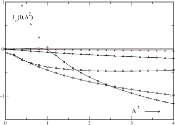
Figure 1: Dependence of the partial wave functional determinant on the cutoff: small $\Lambda$; we display the quantity $J_{n}(0,\Lambda^{2})$ as a function of $\Lambda^{2}$. The solid lines are the results of the Green’ s function approach, the symbols are those of the Gel’fand-Yaglom method; squares: $n=0$; diamonds: $n=1$, circles: $n=2$; triangles: $n=5$, crosses: $n=10$.

The methods of computing the fluctuation determinants has been described in the previous sections, this discussion already incorporates the numerical procedure. We have compared the two methods for computing functional determinants analytically. Of course this should reflect itself in the numerical computations. The quantity to be computed and compared is $J_{n}(0,\Lambda^{2})$ and its partial wave sum ${\cal J}(0,\Lambda^{2})$. In the following we just display results for $n\geq 0$, of course those for $-n$ are identical to those for $n$.

In Figure 1 we display the contributions of various partial waves $J_{n}(0,\Lambda^{2})$ for small $\Lambda^{2}$. The results of the Green’s function method and of the Gel’fand-Yaglom method agree within drawing accuracy, and in fact to better than $1\%$ for all values. A difference is found for the $n=1$ partial wave, due to our translation mode subtraction; the result are expected to agree for $\Lambda^{2}>1$, and they do. The singularity at small $\Lambda^{2}$ found in the Gel’fand-Yaglom results (diamonds) is due to the fact that the translation mode is removed from $J_{n}(0)$ but not from $J_{n}(\Lambda^{2})$; this is correct.

In Figure 2 we again display the quantity $J_{n}(0,\Lambda^{2})$, this time for large $\Lambda$. In these results, as in the ones of the previous figure the first order perturbative contribution is not yet subtracted. So neither of the contributions is expected to have a finite limit as $\Lambda^{2}\to\infty$, they should behave as $\ln\Lambda^{2}$. One sees that the $s$ wave, $n=0$ contribution changes sign and evolves in the positive direction, opposite to the other ones.

If one subtracts the first order perturbative contribution the picture changes, as displayed in Figure 3. Now all partial waves with $n\neq 0$ have finite limits as $\Lambda^{2}\to\infty$, but not so the one with $n=0$. This is the manifestation of the $s$ wave problem. At finite $\Lambda^{2}$ the sum over partial waves is convergent, and in the limit $\Lambda^{2}\to\infty$ the singular behaviour of the $s$-wave is compensated by the other partial waves.

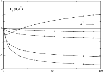
Figure 2: Dependence of the partial wave functional determinant on the cutoff: large $\Lambda$; we display the quantity $J_{n}(0,\Lambda^{2})$ as a function of $\Lambda^{2}$. The solid lines are the results of the Green’ s function approach, the symbols are those of the Gel’fand-Yaglom method; squares: $n=0$; diamonds: $n=1$, circles: $n=2$; triangles: $n=5$, crosses: $n=10$.

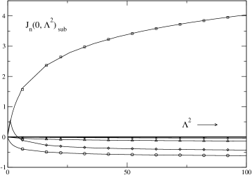
Figure 3: Dependence of the partial wave functional determinant on the cutoff: large $\Lambda$; we display the quantity $J_{n}(0,\Lambda^{2})$ as a function of $\Lambda^{2}$ after subtraction of the first perturbative order. The lines and symbols refer to the same partial waves in the previous figure.

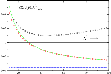
Figure 4: Cutoff dependence of partial wave sums: the sums $1/2\Sigma_{n}J_{n}(0,\Lambda^{2})_{sub}$ as a function of $\Lambda^{2}$; circles: summation up to $\bar{n}=35$, squares: extrapolated sums; solid line: the fit $-.353+1.037/\Lambda^{2}$, dashed line: asymptotic value $-.353$. The sums include the Faddeev-Popov contributions.

Having computed the quantities $J_{n}(0,\Lambda^{2})_{sub}$ we have to do the sum over partial waves and then let $\Lambda^{2}\to\infty$. We find that the terms $J_{n}(0,\Lambda^{2})_{sub}$ behave as $n^{-3}$ for the gauge-Higgs system and as $n^{-5}$ for the Faddeev-Popov system. If the terms have been computed up to some $\bar{n}$, we extrapolate by fitting the terms $\bar{n}-5$ to $\bar{n}$ to $An^{-3}+Bn^{-4}+Cn^{-5}$ and $An^{-5}+Bn^{-6}+Cn^{-6}$, respectively. Then we append the sum from $\bar{n}+1$ to $\infty$ using this fit. This procedure has been used in previous publications, it has been checked here by varying $\bar{m}$ between $20$ and $35$ to give reliable results. The sums up to $n=35$ and the extrapolated sums are plotted in Fig. 4 for $10<\Lambda^{2}<100$. Here the Faddeev-Popov contributions are included. Obviously neither of these are independent of $\Lambda^{2}$. The sum with the fixed upper limit $\bar{n}=35$ first decreases and then starts to increase. This is a consequence of the cancellation of the $s$-wave divergence by the other partial waves. As $\Lambda^{2}$ increases, more and more partial waves are necessary for this compensation, so with a fixed number of partial waves this cannot work. The extrapolated sum is not constant either, but it can be fitted to a behaviour $S_{\infty}+c/\Lambda^{2}$. Subasymptotic corrections of order $1/\Lambda^{2}$ are expected. We consider the number $S_{\infty}$ as the asymptotic value, to be identified with the effective action. It is obvious that the cancellation between the $s$-wave and the higher partial waves becomes more an more delicate if $\Lambda^{2}$ increases, so it is not suitable to choose even higher values of $\Lambda^{2}$ to get a better estimate for $S_{\infty}$.

The results for the effective action

$$S_{eff}=\lim_{\Lambda^{2}\to\infty}\frac{1}{2}J_{n}(0,\Lambda^{2})_{sub}$$ (6.1)

found by the procedure we have described above are displayed in Fig. 5. We also plot the results obtained in our previous publication with Torsten Daiber [19]. These results are consistent with the present ones within the error of $0.07$ estimated in Ref. [19], except for the value at $\xi=.4$. We do not intend to give a detailed error estimate here. From varying the maximal value of the angular momentum and the cutoffs we think that the error is around $0.01$, i.e. within “drawing accuracy”. The Green’s function and Gel’fand-Yaglom methods produce consistent results within an error margin of better than $1\%$. However we still have to rely on extrapolations, and this produces some uncertainty, which may be systematic.

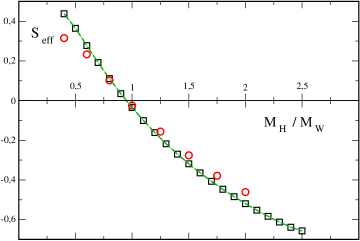
Figure 5: The effective action; squares: our results; circles: the results of Ref. [19].

An interesting problem appears when $\xi=M_{H}/M_{W}>2$. The nondiagonal terms $V_{34}=V_{43}$ behave as $\exp(-M_{W}r)$. So if $f^{\alpha-}_{3}(r,\nu^{2})\simeq exp(-\kappa_{W}r)$ it contributes with a behaviour $\exp(-(\kappa_{W}+M_{W})r$ to $f^{\alpha-}_{4}(r,\nu^{2})$. Now $f^{\alpha-}_{4}$ is supposed to behave as $\exp(-\kappa_{H}r)$. The cross term dominates over this behaviour for $\nu^{2}<M_{H}^{2}(M_{H}^{2}-4M_{W}^{2})/4M_{W}^{2}$. This defines a real interval for $\nu$ if $M_{H}>2M_{W}$. It found indeed that for $M_{H}>2M_{W}$ and small $\nu^{2}$ some of the functions $h^{\alpha-}_{i}$ increase exponentially with the expected behaviour. One finds (numerically) that these contributions cancel in the determinant, both methods still produce consistent results up to $\xi=M_{H}/M_{W}\simeq 2.5$. However, this cancellation is delicate numerically and for larger values $\xi$ the numerical procedure breaks down, the results become inconsistent. So one would have to find a suitable modification of the numerical procedure in order to maintain numerical reliability, here we limit ourselves to the range $\xi<2.5$.

7 Summary

In this work we have addressed a problem that arises in the fluctuation operator and in functional determinant for external field configurations with nontrivial winding number. A modification of the centrifugal barrier factors $n_{i}^{2}/r^{2}$ by the singular external field configuration necessitates modifications in the computation of functional determinants. While these are relatively trivial when the computation is carried out using the Green’s function method, for the Gel’fand-Yaglom they are less obvious. We have described here both approaches. Indeed the handling of the problem when using the Green’s function method has led us to the solution of the problem for the Gel’fand-Yaglom method. It consists in introducing a cutoff, which before was unnecessary after suitable perturbative subtraction.

We have presented the numerical comparison of both methods, the results are found to agree within an accuracy of better than $1\%$. The results for the one-loop effective action agree with the previous calculation in Ref. [19] within the errors given there.

Appendix A The Bais-Primack method

We shortly address the problem of finding reliable classical solutions for the vortex background field. As we have already mentioned, we use a method developed by Bais and Primack [30], which has to be adapted to the vortex system.

We introduce two functions $F_{A}(x)$ and $F_{f}(x)$ with $x=M_{W}r$ via

$$A(r) = -1+xF_{A}(x)$$ (A.1)

$$f(r) = 1+F_{f}(x)\;\;.$$ (A.2)

The boundary condition for these new functions are that $f_{A}(x)\to 0$ and $F_{f}(x)\to 0$ as $x\to\infty$. For $x\to 0$ they have to behave as $f_{A}(x)=1/x+O(x)$ and $F_{f}(x)=-1/x+O(x)$. They satisfy the differential equations

$$F_{A}^{\prime\prime}+\frac{1}{x}F_{A}^{\prime}-\frac{1}{x^{2}}F_{A}-F_{A} = F_{A}(F_{f}^{2}-2F_{f})$$ (A.3)

$$F_{f}^{\prime\prime}+\frac{1}{x}F_{f}^{\prime}-\xi^{2}F_{f} = F_{A}^{2}(1+F_{f})+\frac{\xi^{2}}{2}F_{f}^{2}(3+F_{f})\;\;.$$ (A.4)

which have been written in such a way that the differential operators on the left hand side

$${\cal D}_{A} = \frac{d^{2}}{dx^{2}}+\frac{1}{x}\frac{d}{dx}-\frac{1}{x^{2}}-1$$ (A.5)

$${\cal D}_{f} = \frac{d^{2}}{dx^{2}}+\frac{1}{x}\frac{d}{dx}-\xi^{2}$$ (A.6)

are of the Bessel type. Their Green’ s functions are given by

$$G_{A}(x,x^{\prime}) = I_{1}(x_{<})K_{1}(x_{>})$$ (A.7)

$$G_{f}(x,x^{\prime}) = I_{0}(\xi x_{<})K_{0}(\xi x_{>})$$ (A.8)

and we have the integral equations

$$F_{A}(x) = F_{A}^{0}(x)-\int_{0}^{\infty}xdxG_{A}(x,x^{\prime})\left[F_{A}(x^{\prime})(F_{f}^{2}(x^{\prime})+2F_{f}(x^{\prime}))\right.$$

$$\left.-{\cal D}_{A}F_{A}^{0}(x^{\prime})\right]$$

$$F_{f}(x) = F_{f}^{0}(x)-\int_{0}^{\infty}xdxG_{f}(x,x^{\prime})\left[F_{A}^{2}(x^{\prime})(1+F_{f}(x^{\prime})\right.$$

$$\left.+\frac{\xi^{2}}{2}F_{f}^{2}(x^{\prime})\left(3+F_{f}(x^{\prime})\right)-{\cal D}_{f}F_{f}^{0}(x^{\prime})\right]\;\;.$$

The functions $F_{f}^{0}$ und $F_{A}^{0}$ have been introduced in order to provide the solutions with the right boundary conditions. They have to satisfy the same boundary conditions as the solutions we are looking for. We have chosen

$$F_{A}^{0}(x) = K_{1}(x)\frac{1+a_{1}x}{1+a_{2}x}$$ (A.11)

$$F_{f}^{0}(x) = -K_{1}(\xi x)\frac{\xi x}{1+f_{1}x}\;\;.$$ (A.12)

with suitable parameters $a_{1},a_{2}$ and $f_{1}$ the iteration of the integral equations produces solutions with an accuracy of $10^{-9}$ after around $150$ iterations.

Appendix B Coleman’s proof of the Gel’fand-Yaglom theorem

In the book by Coleman [5] the Gel’fand-Yaglom theorem is stated in the following way: Let $f(r,\nu^{2})$ and $f^{0}(r,\nu^{2})$ denote the solutions of

$$({\bf M}+\nu^{2})f(r,\nu^{2})=0$$ (B.1)

and

$$({\bf M}^{0}+\nu^{2})f^{0}(r,\nu^{2})=0\;,$$ (B.2)

respectively, on the interval $[0,\infty]$, with regular boundary conditions at $r=0$. Let these solutions be normalized such that

$$\lim_{r\to 0}\frac{f(r,\nu^{2})}{f^{0}(r,\nu^{2})}=1\;.$$ (B.3)

Then the following equality holds:

$$\frac{\det({\bf M}+\nu^{2})}{\det({\bf M}^{0}+\nu^{2})}=\lim_{r\to\infty}\frac{f(r,\nu^{2})}{f^{0}(r,\nu^{2})}\;\;.$$ (B.4)

The argument consists of two parts:
(i) as the bound state condition for the functions $f(r,\nu^{2})$ and $f^{0}(r,\nu^{2})$ is given by $f(\infty,-\omega_{\alpha}^{2})=0$ and $f^{0}(\infty,-{\omega_{\alpha}^{0}}^{2})=0$, and as the determinants can be written, in the basis of eigenstates, as products with factors $\nu^{2}+\omega_{\alpha}^{2}$ and similarly for the determinant of ${\bf M}^{0}+\nu^{2}$ the right hand and left hand sides are meromorphic functions with identical poles and zeros.
(ii) therefore, if furthermore both sides become unity as $\nu^{2}\to\infty$, they are identical. This condition holds for a large class of potentials, in particular nonsingular potentials of finite range. Intuitively one expects that for large $\nu^{2}$ the potential then becomes irrelevant and that the solutions $f(r,\nu^{2})$ and $f^{0}(r,\nu^{2})$ become identical, the condition my be checked by perturbative expansion.

Generalized to a coupled $(n\times n)$ system the theorem can be stated in the following way:

Let ${\bf f}(r,\nu^{2})$ and ${\bf f}^{0}(r,\nu^{2})$ denote the $(n\times n)$ matrices formed by $n$ linearly independent solutions $f_{i}^{\alpha}(r,\nu^{2})$ and $f_{i}^{\alpha 0}(r,\nu^{2})$ of

$$({\bf M}_{ij}+\nu^{2})f_{j}^{\alpha}(r,\nu^{2})=0$$ (B.5)

and

$$({\bf M}_{ij}^{0}+\nu^{2})f^{\alpha 0}_{j}(r,\nu^{2})=0\;,$$ (B.6)

respectively, with regular boundary conditions at $r=0$. The lower index denotes the $n$ components, the different solutions are labelled by the Greek upper index. Let these solutions be normalized such that

$$\lim_{r\to 0}{\bf f}(r,\nu^{2})({\bf f}^{0}(r,\nu^{2}))^{-1}={\bf 1}\;.$$ (B.7)

Then the following equality holds:

$$\frac{\det({\bf M}+\nu^{2})}{\det({\bf M}^{0}+\nu^{2})}=\lim_{r\to\infty}\frac{\det{\bf f}(r,\nu^{2})}{\det{\bf f}^{0}(r,\nu^{2})}$$ (B.8)

where the determinants on the left hand side are determinants in functional space, those on the right hand side are ordinary determinants of the $n\times n$ matrices defined above.

The argument goes as before, one just has to replace the bound state condition for the one-channel problem by the condition

$$\lim_{r\to\infty}\det{\bf f}(r,\nu^{2})=0$$ (B.9)

as suited for a coupled-channel problem.

Appendix C Gel’fand-Yaglom and the Green’s function

In section 4 we have have introduced two numerical methods for computing the functional determinant of an operator ${\cal M}$, or rather of operators ${\bf M}_{n}$, the reduction of the operator ${\cal M}$ to a subspace of definite angular momentum. We will here connect the two methods directly, without going back to the eigenfunctions of this operator which are not used in either of the methods. The connection between the methods has been discussed in Ref. [32], we adapt their aproach to the radial and coupled-channel operators which we have consider here.

We go back to the diffential equation satisfied by the mode functions $f^{\pm}(r,\kappa)$

$$\left[-\frac{1}{r}\frac{d}{dr}r\frac{d}{dr}+\frac{n^{2}}{r^{2}}+V(r)+\nu^{2}\right]f_{n}^{\pm}{r,\nu^{2}}=0$$ (C.1)

Taking the derivative with respect to $\nu^{2}$ of the differental equation for $f^{-}_{n}$ we have

$$\left[-\frac{1}{r}\frac{d}{dr}r\frac{d}{dr}+\frac{n^{2}}{r^{2}}+V(r)+\nu^{2}\right]\frac{d}{d\nu^{2}}f_{n}^{-}(r,\nu^{2})+f_{n}^{-}(r,\nu^{2})=0$$ (C.2)

Multiplying with $f^{+}(r,\nu^{2})$ and using the differential equation for $f_{n}^{+}$ we obtain

$$\left[\frac{1}{r}\frac{d}{dr}r\frac{d}{dr}f^{+}(r,\nu^{2})\right]\frac{d}{d\nu^{2}}f_{n}^{-}(r,\nu^{2})-f^{+}(r,\nu^{2})\frac{d}{d\nu^{2}}\frac{1}{r}\frac{d}{dr}r\frac{d}{dr}f^{-}(r,\nu^{2})$$

$$=-f_{n}^{+}(r,\nu^{2})f_{n}^{-}(r,\nu^{2})=-{\bf G}_{n}(r,r,\nu^{2})$$ (C.3)

Integrating the Green’s function over $r$ we have

$$-\int_{0}^{\infty}rdr{\bf G}_{n}(r,r,\nu^{2})=$$

$$=-\int_{0}^{\infty}rdr\frac{1}{r}\frac{d}{dr}\left\{\left[r\frac{d}{dr}f_{n}^{+}(r,\nu^{2})\right]\frac{d}{d\nu^{2}}f_{n}^{-}(r,\nu^{2})-f_{n}^{+}(r,\nu^{2})\frac{d}{d\nu^{2}}r\frac{d}{dr}f_{n}^{-}(r,\nu^{2})\right\}$$

$$=\left\{\left[r\frac{d}{dr}f_{n}^{+}(r,\nu^{2})\right]\frac{d}{d\nu^{2}}f_{n}^{-}(r,\nu^{2})-f_{n}^{+}(r,\nu^{2})\frac{d}{d\nu^{2}}r\frac{d}{dr}f_{n}^{-}(r,\nu^{2})\right\}\biggl{|}_{0}^{\infty}$$ (C.4)

In fact we have to compute the integral over ${\bf G}_{n}-{\bf G}_{0,n}$ and with the boundary conditions and normalization we have introduced the contributions of the two Green’s functions cancel each other at the upper integration limit. Near the lower integration limit the functions $f^{\pm}_{n}(r,\nu^{2})$ behave as $(1+h^{+}_{n}(r,\nu^{2}))K_{n}(\kappa r)$ and $(1+h^{-}_{n}(r,\nu^{2}))I_{n}(\kappa r)$ with $\lim_{r\to 0}(1+h_{n}^{+}(r,\nu^{2}))(1+h_{n}^{-}(r,\nu^{2}))=1$. Therefore the parts where the derivatives $d/d\nu^{2}$ act on the Bessel functions cancel with the free contribution and we remaining term is given by

$$-(1+h^{+}_{n}(0,\nu^{2}))\frac{d}{d\nu^{2}}(1+h^{-}_{n}(0,\nu^{2})w(K_{n}(\kappa r),I_{n}(\kappa r))$$

$$=\frac{dh^{-}_{n}(0,\nu^{2})/d\nu^{2}}{1+h^{-}_{n}(0,\nu^{2})}=\frac{d}{d\nu^{2}}\ln\left[1+h^{-}_{n}(0,\nu^{2})\right]\;\;,$$ (C.5)

where we have used

$$w(K_{n}(z)I_{n}(z))\equiv z\left[I_{n}(z)\frac{d}{dz}K_{n}(z)-K_{n}(z)\frac{d}{dz}I_{n}(z)\right]=-1\;\;.$$ (C.6)

In subsection 4.2 we have introduced the functions $\tilde{f}^{-}_{n}(r,\nu^{2})$ which differ from the $f^{-}_{n}$ in the normalization. Writing

$$\tilde{f}^{-}_{n}(r,\nu^{2})=I_{n}(\kappa r)\left[1+\tilde{h}^{-}_{n}(r,\nu^{2})\right]$$ (C.7)

we have

$$1+h_{n}^{-}(0,\nu^{2})=\frac{1}{1+\tilde{h}_{n}^{-}(\infty,\nu^{2})}$$ (C.8)

So we obtain

$${\bf J}_{n}(\nu^{2},\Lambda^{2}) = -\int_{\nu^{2}}^{\Lambda^{2}}d\nu^{{}^{\prime}2}\left[{\bf G}_{n}(\nu^{{}^{\prime}2})-{\bf G}_{0,n}(\nu^{{}^{\prime}2})\right]$$ (C.9)

$$= \int_{\nu^{2}}^{\Lambda^{2}}d\nu^{{}^{\prime}2}\frac{d}{d\nu^{{}^{\prime}2}}\ln\left[1+h^{-}_{n}(0,\nu^{{}^{\prime}2})\right]$$ (C.10)

$$= \ln\left[1+h^{-}_{n}(0,\nu^{{}^{\prime}2})\right]\biggl{|}_{\nu^{2}}^{\Lambda^{2}}$$ (C.11)

$$= -\ln\left[1+{\tilde{h}}^{-}_{n}(\infty,\nu^{{}^{\prime}2})\right]\biggl{|}_{\nu^{2}}^{\Lambda^{2}}$$ (C.12)

$$= \ln\frac{1+\tilde{h}^{-}_{n}(\infty,\nu^{2})}{1+\tilde{h}^{-}_{n}(\infty,\Lambda^{2})}$$ (C.13)

Generalizing to coupled channels, choosing the Wronskian derterminant $\omega^{\alpha\beta}=\delta^{\alpha\beta}$ we have

$$-\int_{0}^{\infty}rdr{\bf G}_{n,ii}(r,r,\nu^{2})=$$ (C.14)

$$=\left\{\left[r\frac{d}{dr}f_{n,i}^{\alpha+}(r,\nu^{2})\right]\frac{d}{d\nu^{2}}f_{n,i}^{\alpha-}(r,\nu^{2})-f_{n,i}^{\alpha+}(r,\nu^{2})\frac{d}{d\nu^{2}}r\frac{d}{dr}f_{n}^{\alpha-}(r,\nu^{2})\right\}\biggl{|}_{0}^{\infty}$$

The subsequent reasoning about the contributions of the upper and lower integration limit is analogous. We now have

$$-(1+h^{\alpha+}_{ni}(0,\nu^{2}))\frac{d}{d\nu^{2}}(1+h^{\alpha-}_{ni}(0,\nu^{2})w(K_{n_{i}}(\kappa r),I_{n_{i}}(\kappa r))$$

$$=\left[{\bf I}+{\bf h}^{-}_{n}(0,\nu^{2})\right]^{-1}\frac{d{\bf h}^{-}_{n}(0,\nu^{2})}{d\nu^{2}}=\frac{d}{d\nu^{2}}\ln\det\left[{\bf I}+{\bf h}^{-}_{n}(0,\nu^{2})\right]\;\;.$$ (C.15)

and by analogous steps as for the single-channel case we arrive at

$${\bf J}_{n}(0,\Lambda^{2}) = -\int_{0}^{\Lambda^{2}}d\nu^{2}\left[{\bf G}_{n,ii}(\nu^{2})-{\bf G}_{0,n,ii}(\nu^{2})\right]$$ (C.16)

$$= \int_{0}^{\Lambda^{2}}d\nu^{2}\frac{d}{d\nu^{2}}\ln\det\left[{\bf I}+{\bf h}^{-}_{n}(0,\nu^{2})\right]$$

$$= \ln\frac{\det{\left[{\bf I}+{\bf\tilde{h}}^{-}_{n}(0,0)\right]}}{\det{\left[{\bf I}+{\bf\tilde{h}}^{-}_{n}(0,\Lambda^{2})\right]}}$$

As we will see it is not always possible to normalize the fundamental system at $r=0$. A more general expression, which treats the boundaries $r=0$ and $r\to\infty$ in a symmetrical way is given by

$${\bf J}_{n}(0,\Lambda^{2})=\ln\frac{\det{\left[{\bf I}+{\bf\hat{h}}^{-}_{n}(\infty,0)\right]}\det{\left[{\bf I}+{\bf\hat{h}}^{-}_{n}(0,\Lambda^{2})\right]}}{\det{\left[{\bf I}+{\bf\hat{h}}^{-}_{n}(\infty,\Lambda^{2})\right]}\det{\left[{\bf I}+{\bf\hat{h}}^{-}_{n}(0,0)\right]}}\;\;,$$ (C.17)

where now the matrix ${\bf\hat{h}}=\{\hat{h}^{\alpha}_{n}\}$ refers to a fundamental system with an arbitrary normalization.

References

• [1] I. Gel’fand and A. Yaglom, J. Math. Phys. 1, 48 (1960).
• [2] J. van Vleck, Proc. Nat. Acad. Sci. 14, 178 (1928).
• [3] R. Cameron and T. Martin, Am. Math. Soc. 51, 73 (1945).
• [4] R. Dashen, B. Hasslacher and A. Neveu, Phys. Rev. D10, 4114 (1974).
• [5] S. Coleman, Aspects of Symmetry (Cambridge University Press, 1985).
• [6] J. Baacke and G. Lavrelashvili, Phys. Rev. D69, 025009 (2004), [hep-th/0307202].
• [7] K. Kirsten and A. J. McKane, Annals Phys. 308, 502 (2003), [math-ph/0305010].
• [8] K. Kirsten and A. J. McKane, J. Phys. A37, 4649 (2004), [math-ph/0403050].
• [9] Y. Burnier and M. Shaposhnikov, Phys. Rev. D72, 065011 (2005), [hep-ph/0507130].
• [10] G. V. Dunne and H. Min, Phys. Rev. D72, 125004 (2005), [hep-th/0511156].
• [11] G. V. Dunne and K. Kirsten, J. Phys. A39, 11915 (2006), [hep-th/0607066].
• [12] G. V. Dunne, J. Hur, C. Lee and H. Min, Phys. Rev. D77, 045004 (2008), [arXiv:0711.4877 [hep-th]].
• [13] V. G. Kiselev and K. G. Selivanov, JETP Lett. 39, 85 (1984).
• [14] V. Kiselev and K. Selivanov, Sov. J. Nucl. Phys. 43, 153 (1986).
• [15] K. G. Selivanov, Sov. Phys. JETP 67, 1548 (1988).
• [16] J. Baacke and V. G. Kiselev, Phys. Rev. D48, 5648 (1993), [hep-ph/9308273].
• [17] J. Baacke, Phys. Rev. D52, 6760 (1995), [hep-ph/9503350].
• [18] A. Surig, Phys. Rev. D57, 5049 (1998), [hep-ph/9706259].
• [19] J. Baacke and T. Daiber, Phys. Rev. D51, 795 (1995), [hep-th/9408010].
• [20] J. Baacke and S. Junker, Phys. Rev. D49, 2055 (1994), [hep-ph/9308310].
• [21] J. Baacke and S. Junker, Phys. Rev. D50, 4227 (1994), [hep-th/9402078].
• [22] D. Y. Grigoriev, V. A. Rubakov and M. E. Shaposhnikov, Phys. Lett. B216, 172 (1989).
• [23] W. H. Tang and J. Smit, Nucl. Phys. B540, 437 (1999), [hep-lat/9805001].
• [24] A. I. Bochkarev and M. E. Shaposhnikov, Mod. Phys. Lett. A2, 991 (1987).
• [25] A. I. Bochkarev and G. G. Tsitsishvili, Phys. Rev. D40, 1378 (1989).
• [26] H. B. Nielsen and P. Olesen, Nucl. Phys. B61, 45 (1973).
• [27] H. J. de Vega and F. A. Schaposnik, Phys. Rev. D14, 1100 (1976).
• [28] N. K. Nielsen and B. Schroer, Nucl. Phys. B120, 62 (1977).
• [29] N. K. Nielsen and B. Schroer, Nucl. Phys. B127, 493 (1977).
• [30] F. A. Bais and J. R. Primack, Phys. Rev. D13, 819 (1976).
• [31] J. Kripfganz and A. Ringwald, Mod. Phys. Lett. A5, 675 (1990).
• [32] H. Kleinert and A. Chervyakov, Phys. Lett. A245, 345 (1998), [quant-ph/9803016].