The Universe as an Inside-Out Star

Abstract

Acoustic modes can be used to study the physics of the interior of a cavity, and this is especially useful when the inside region is inaccessible. Many astrophysicists use such sound waves as an essential tool in their research. Here we focus on two separate sub-fields in which oscillations on the surface of a sphere are studied – Helioseismology and CMBology – the surface being either the solar or cosmic photosphere. Both research areas use the language of spherical harmonics, as well as sharing many close similarities in the underlying physics. However, there are also many fundamental differences, which we explain in this pedagogical article.

I Introduction

‘CMBology’ (or CMB-Cosmology), the study of temperature fluctuations in the Cosmic Microwave Background (CMB cmb ), and Helioseismology, the study of acoustic oscillations on the surface of the Sun helio , are two fields of much experimental and theoretical interest today. In the last decade, our knowledge of both areas has increased dramatically through an active ground and space-based observational programme. This has led to substantial improvement in the quantification of models for both the early Universe and the interior of the Sun, and hence given us a deeper understanding of the underlying physics.

These two areas are vastly different in terms of scale. Firstly, consider the difference in physical size. Cosmology – literally ‘the study of the whole Universe’ – encompasses scales so vast as to make even our own Galaxy seem minuscule. The study of solar oscillations, on the other hand, is constrained to an object barely 100 Earths in diameter – virtually non-existent on a cosmological map. We can also consider the vast temporal disparity between the two fields. The photons we observe from the Sun describe it as it was about 8 minutes ago, while CMB photons give an imprint of the Universe as it was more than 13 billion years ago.

Although the Sun and CMB are very different in terms of scale, the underlying physics enabling us to understand them is essentially the same – the physics of sound waves resonating in a cavity. Acoustic waves are a common everyday physical phenomenon, and every undergraduate learns about the use of standing sound waves to understand the interior of a cavity. Probing the same kinds of waves in the early Universe and solar interior is of great importance, since they can be used to study the insides of objects which are otherwise unreachable.

In this article we will compare the physics of these 2 astrophysical arenas: CMB anisotropies and and helioseismology. Both use similar language, talking about acoustic modes, the photosphere and spherical harmonics, and hence it should come as no surprise that there are very close physical analogues which can be drawn. However, as we will see, this is only possible if one thinks about the Universe as an inside-out version of a star.

II The CMB and Helioseismology

II.1 Standard Cosmological Model

All current cosmological data point towards the Hot Big Bang picture, in which the early Universe was full of relativistic particles (baryons and electrons) and radiation, along with components of dark matter and dark energy. This extremely dense and hot Universe evolved by expanding and cooling – as does an expanding gas. Most of the initial energy was in radiation, which drove the expansion according to the equations of General Relativity. Because of the expansion, radiation from earlier times reaches us with stretched wavelengths, and it is natural to use the observed redshift, $z$, as a label for the epoch we are observing – $z$ increases monotonically as we look farther away and back to earlier times.

The immensely high temperatures meant that photons – whose energy distributions well approximated a black-body spectrum – were originally energetic enough to keep the atoms ionized. The primordial gas, then, must have been optically thick, due to the high cross-section for Thomson scattering of the free electrons. Photons and baryons were said to be ‘coupled’ during this era; the continuous scattering off one another linked their temperature and fluid properties.

As the Universe cooled, the rate of expansion fell due to the overall gravitational attraction of matter. A number of important epochs occurred as particle interaction rates fell below the expansion rate. One example is the formation of the light elements at a temperature of around $1\,$MeV (redshift of several billion), as the conversion between neutrons and protons froze out. This gave a helium mass fraction of around 25%, in fairly close agreement with the value in the solar interior today.

As the Universe continued to cool, the ratio of the energy density in massive particles relative to radiation increased, until the epoch of matter-radiation equality was reached. At a redshift several times smaller than this ($z\,{\simeq}\,1000$), very few photons were energetic enough to ionize hydrogen, and so electrons were captured by protons, leading to an optically thin universe – a process referred to as cosmological recombination. Photons, having been freed from their electron captors travelled unhindered through a mostly empty space until they are seen today as the CMB. The probability for a photon last scattering with an electron peaks at $z\,{\simeq}\,1100$, and so we call this the ‘last scattering surface’.

Photons which last scattered at this epoch are seen today with a remarkably pure black-body distribution at a cool temperature of about $2.7\,$K. At a redshift of 1100 this means that recombination occurred at a temperature of about $3000\,$K. This cosmic photosphere is seen at an age of around 400,000 years, while the age of the Universe today is about 14 billion years.

The background radiation, as seen by any observer, is remarkably isotropic, but contains the signatures of primordial structure in the form of temperature anisotropies on the order of one part in $10^{5}$. It is these anisotropies which are of most interest to cosmologists, as their measurement promises to constrain the many otherwise free parameters in theoretical models of the evolution of the Universe. Moreover, they are caused by the small fluctuations in density which grow in contrast to become the rich structure (galaxies, stars, people) that we see today.

II.2 Standard Solar Model

Not unlike the CMB, the solar surface is mostly uniform. When we observe the Sun, we see photons escaping from the solar photosphere, the energy distribution of which is crudely that of a black-body with an effective temperature $T\,{\simeq}\,5800\,$K. Because of its brightness and angular extent on our sky, solar temperature anisotropies were witnessed long before scientific explanation could be provided for them. Sunspots were first noted by Galileo and could be seen with a tool as simple as a pin-hole camera. However, these large solar ‘blemishes’ are very localized on the solar surface, as well as being transient, and as such do not contribute much to the overall variance of angular anisotropies; in CMB language, sunspots are localized highly non-Gaussian cold spots with amplitude $\Delta T/T\simeq 0.1$.

The configuration of the solar interior can be inferred by applying the standard equations of stellar structure, which derive from the principles of thermal and hydrostatic equilibrium. These are complicated by details of energy generation through nuclear processes and energy transport by radiation and convection. The convective zone is confined to the outer 30$\%$ of the solar radius, where no radiative transport occurs. Energy generation is driven by the conversion of hydrogen to helium at similar temperatures to what was achieved in the Universe when the primordial helium was formed.

It is the acoustic oscillations – anisotropies discovered in 1960 by observing Doppler shifts in absorption lines due to the physical movements of atoms in the photosphere – which are of greatest interest to helioseismologists. These oscillations, composed of various pressure modes or ‘p-modes’, are waves sustained by a radial pressure gradient; they are sound waves trapped in the solar interior. The principle underlying helioseismology is that the various acoustic modes provide different information about the solar interior. In particular, modes characterized by different numbers of radial nodes penetrate to different depths within the Sun, providing a series of probes allowing one to determine the radially dependent physics of the Sun. For example, by measuring the dispersion relation of a mode, one can estimate the average sound speed it experiences. Using several modes, and knowing their penetration depths, a helioseismologist can determine the functional form of the solar sound speed with respect to radius. Such tests can be used to both confirm and to constrain parameters within the Standard Solar Model, including determining the interior composition and rotation rate.

II.3 The Universe as an inside-out star

Some similarities between the Sun and the Universe should already be apparent. Consider, for instance, that an observation of either the CMB or the Sun collects photons originating from a spherical surface, and describing a nearly uniform black-body spectrum. In the Sun the photosphere is the surface where gas density has increased sufficiently for photons to be strongly scattered, and its radius is usually defined as $R_{\odot}$, which is around $700{,}000\,$km. In the CMB the last scattering surface has a distance from the Big Bang which is given by the recombination time times the speed of light. However, the CMB sky surrounds us, and when we look out towards the cosmic photosphere it is like looking into the surface of a star.

In contrast, the Sun is localized on our sky. That is to say, one can point a finger at the centre of the Sun with the knowledge that it is entirely contained within some finite radius of that point (at a given time). This is not possible for the CMB last scattering surface, where every observer (potentially in quite different parts of the Universe) has their own last scattering surface. This is because in the uniformly expanding Universe everything is moving away from everything else – thus there is no true centre of the universal expansion or, rather, every point can be considered to be the centre. So every observer sees the early Universe photons arriving from all directions in a spherical shell around them. We are at the centre of a space in which the cosmic photosphere surrounds us, as if the surface of the star had been wrapped all round us. The centre of this ‘star’ is then located in the very early Universe, well beyond the distance of the last scattering surface, and this centre (the position of the ‘Big Bang’ if you like) is in every direction as we look out, into the ‘cosmic star’.

The Solar and Cosmic photospheres are therefore quite analogous to each other. It is the fluctuations over each of these spheres which are of most interest, since they probe the nature of the acoustic cavities. Helioseismologists and cosmologists use the same mathematical tools to describe these acoustic modes, namely the spherical harmonics. Any angular function $f(\theta,\phi)$ can be expanded in terms of spherical harmonics by

$$f(\theta,\phi)=\sum_{\ell=0}^{\infty}\sum_{-\ell}^{\ell}a_{\ell m}Y_{\ell m}(\theta,\phi)\,.$$ (1)

Several of these modes are illustrated in Fig 1. Roughly speaking, the $\ell$ index describes the angular extent of features, $\simeq 180^{\circ}/\ell$, while $m$ characterizes the azimuthal dependence. Cosmologists are mainly interested in the power spectrum of $a_{\ell m}$s, while helioseismologists study their time dependence. The fact that the Universe is like an inside-out star means there is also another important difference to keep clear. The spherical harmonics describing anisotropies in the Sun and the CMB must be projected from a different centre in each cases – helioseismologists use the centre of the Sun as the origin, while cosmologists use the observer’s position as the centre.

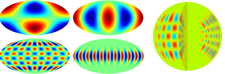
Figure 1: Illustration of the $Y_{\ell m}$ harmonics used to expand the temperature fluctuations of the CMB and velocity fluctuations on the solar surface. In the left panel of four harmonics, we show the real component of: $Y_{2\,1}$ (top-left), $Y_{2\,2}$ (top-right), $Y_{10\,5}$ (bottom-left) and $Y_{10\,10}$ (bottom-right). Cosmologists are interested in the amplitude of these modes, while helioseismologists study their variation with time. Helioseismologists also decompose modes in the third (radial) dimension, as shown on the right.

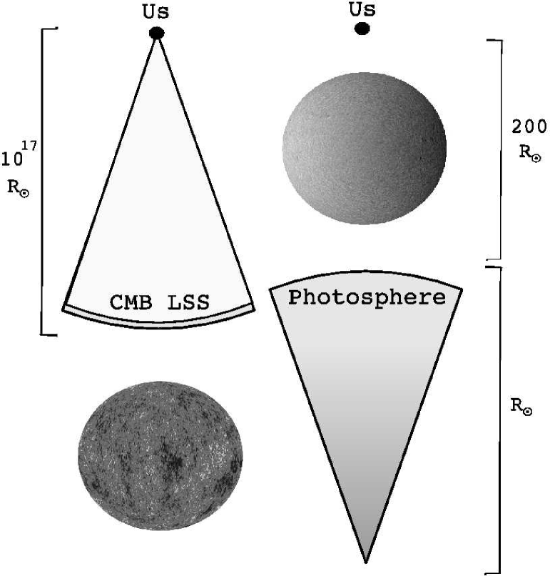
Figure 2: Geometry and length scales of the Sun versus the comic inside-out star.

The scales and ‘inside-out’ geometry are illustrated in Fig. 2. The other major difference is the colossal distance of the cosmic photosphere on which we see the CMB anisotropies. At a redshift of around 1100, the last scattering surface is about $14\,$Gpc away from us (a bit more than the light travel time in 14 billion years, because it has been expanding during that interval). This is about $10^{17}$ times the scale of a Sun-like star. So the Universe is exactly like a star, except that it is completely turned inside-out, and 100 quadrillion times bigger!

II.4 Surface of last scattering and the photosphere

The reason why the inside-out star is an attractive analogy for the CMB is that we observe photons emerging from the cosmic photosphere. This last-scattering surface is a shell defined by the distance from us in which there is a significant probability for the photons to have suffered their last scattering event. We see to where the optical depth $\tau$ is around unity, with $tau$ entirely due to Thomson scattering off free electrons. The last scattering surface is therefore defined by the epoch at which the Universe went from being a plasma to being a neutral gas; the time since this epoch, coupled with the finite speed of light, defines this spherical surface. For the Sun (or any other star) the photosphere is also defined by the region where $\tau\,{\sim}\,1$, but the source of opacity is much more complicated, including lines from heavy elements and $H^{-}$ ion scattering. But there is a more significant distinction, coming from the vastly different photon-to-atom ratio – approximately 1 billion for the Universe, but less than one billionth for the solar surface! Hence the temperature at which the Universe went from plasma to neutral is determined by when the photons allowed the atoms to recombine, and this determines the last-scattering surface. But the photosphere of the Sun is mainly determined by where the density has fallen off. So it is much more like an actual edge to the solar material than in the case of the Universe, where the density is slowly varying, but the ionization changes.

One might then ask why the cosmic recombination temperature turns out to be within a factor of 2 of the temperature of the solar surface. The answer is that partly this was just a coincidence. But the fact that the order of magnitude is similar is not surprising, since this comes basically from the temperature at which atoms get ionized. So, despite the chemistry being different, this is ${\sim}\,$eV in both cases.

Another important feature for the CMB is acoustic damping, which is related to the thickness of the last scattering surface. This turns out to be approximately $\Delta z/z\,{\simeq}\,0.1$, which leads to a smearing of the anisotropies at an angular scale which is about 10 times smaller than the causal scale at the last scattering epoch, corresponding to $\ell\,{\simeq}\,1000$, as can be seen in Fig. 3.

Similarly, in the Sun the optical depth does not drop instantaneously, although it much more abrupt than for the CMB. The thickness of the solar photosphere is a few hundred km or around $0.001\,R_{\odot}$. This means that the damping for solar modes is at an angular scale about 100 times higher in $\ell$ than for the CMB.

III Physics of sound waves

III.1 Acoustic modes

A crucial property of both CMB and solar fluctuations is that their amplitude is small. As a result, the equations which describe them can be solved by linear perturbation theory, such that a set of initial conditions can be evolved forward in time exactly to predict the final observed oscillation spectrum (particularly in the cosmic case), greatly simplifying the comparison of theory with observations.

Both the fluids in the solar interior and early Universe are characterized by several variables, each with an average value and a small perturbation which varies with both time and position – the energy density $\rho$, pressure $P$ (related by an equation of state $P=P(\rho,T)$) and local velocity $v$. A continuity equation enforces conservation of mass, Euler’s equation determines the motion of the fluid, and Poisson’s equation describes the response of the fluid to gravity. The full cosmological equations are relativistic generalizations of these, but the physics is the same.

In order to understand acoustic waves it is sufficient to initially ignore gravity and consider a density perturbation in each fluid. The cosmological fluid is adiabatic, a natural outcome of inflationary initial conditions, and this is also an excellent approximation in most of the solar interior. This means that one can ignore heat exchange between fluid elements – only compression increases the temperature, and expansion cools it. In both cases, the resulting continuity and Euler equations then describe a simple oscillator

$$\ddot{\delta}+\frac{\dot{a}}{a}\dot{\delta}+c_{\rm s}^{2}k^{2}\delta=0\,,$$ (2)

where $\delta\equiv\delta\rho/\rho$, $\delta\rho\ll\rho$ and an overdot denotes the time derivative. The scale factor $a(t)$ describes the cosmological expansion, and is related to redshift by $a=(1+z)^{-1}$ – this term is zero in the solar case. We have written this equation in Fourier space, where $k=2\pi/\lambda$ is the wavenumber of the mode. Neglecting the expansion term, the solution to this equation are plane acoustic waves oscillating at the sound speed, defined through $c_{\rm s}^{2}=dP/d\rho$. In a relativistic cosmological fluid $c_{\rm s}^{2}=c^{2}/3$, where $c$ is the speed a light. In the solar interior the sound speed varies as a function of radius, and for an ideal gas we would just have $c_{\rm s}^{2}=k_{\rm B}T/{\bar{m}}$, where $k_{\rm B}$ is Boltzmann’s constant and ${\bar{m}}$ is the average particle mass. In the standard model of the Sun the values range from about $6\,{\rm km\,s}^{-1}$ near the solar surface to about $500\,{\rm km\,s}^{-1}$ near the solar core.

Equation (2) has several important consequences acoustic . The dispersion relation of the waves, given by $\omega=c_{\rm s}k$, means that spatial and temporal modes are related by a constant in the cosmological fluid – i.e. a wave with twice the wavelength has twice the oscillation timescale, which turns out to be crucial for understanding the observed CMB acoustic spectrum. In the solar interior, the oscillation equations must be combined with boundary conditions at the surface. Coupled with the fact that the sound speed varies as a function of depth, this leads to refraction of waves in the solar interior. High frequency modes are trapped near the surface, while low frequency modes penetrate closer to the core. This means that observation of oscillations as a function of frequency can be used to probe the interior.

Since the oscillations in density in equation (2) also involve oscillations in velocity, then there may be more than one physically observable effect. The velocities will be $90^{\circ}$ out of phase, since the velocity maxima and minima occur at the zeros of the density oscillations. For the Sun it is usually the time-varying Doppler shifts of the velocity oscillations that are observed directly (although there are also luminosity variations observable from the lowest multipole modes). For the CMB the amplitudes of the standing waves are frozen at the last scattering epoch – the main effect is from the density variations, although there is a sub-dominant contribution from the velocities.

Another important property of the acoustic modes is that they are irrotational. This means that the fluid velocity is in the direction of the wavevector k. The cosmological fluid is dominated by irrotational modes, which are the primary source of anisotropy in the CMB. However, inflationary initial conditions also predict a small fraction of rotational modes, which are seeded by gravitational waves. The most characteristic effect of these is through their effect on the pattern of CMB polarization in which (through analogy with curl in electro-magnetism) they are usually referred to as ‘B-modes’. These have not yet been detected, but are one of the main motivations for future CMB missions. In the Sun there is some evidence for ‘r-modes’ in the photosphere, which are similar to the Rossby waves seen in the Earth’s atmosphere and oceans. These are driven by the Sun’s rotation. So, although there is a very loose analogy with the CMB ‘B-modes’, there is also a very fundamental difference – there are extremely strict limits on the rotation of the Universe, coming from the non-observations of spiral-like patterns in the CMB anisotropies.

III.2 Cosmological oscillations

Inflationary cosmology predicts that quantum fluctuations created in the very early Universe seeded gravitational fluctuations within the primordial plasma. The introduction of gravity means that pressure and gravity are now two competing forces. The gravitational instability imposed on these perturbations, along with the counter-acting radiation pressure from the energetic and numerically dense photons (still highly coupled to the baryons) leads to acoustic oscillations within this early plasma.

After recombination, the photons’ restoring radiation pressure no longer drives these oscillations and the perturbations in structure are frozen-out as the CMB is released. On the largest scales we simply see a reflection of the initial conditions in the gravitational potential. This is the main physical effect for angles larger than that subtended by the causal length at last-scattering, which corresponds to about $2^{\circ}$ on the sky (about the width of your thumb held at arm’s length, or coincidentally about 4 times the diameter of the Sun).

On smaller scales, the temperature fluctuations are due to the density and velocity variations in the oscillating plasma at the time of last scattering. One observes these as a ‘fundamental’ mode, together with a series of harmonic overtones in angular scale on the sky. This occurs because of the approximately constant sound speed within the plasma up to decoupling. There therefore exists a scale, which at last scattering had suffered maximal compression – so CMB photons have a maximum temperature variance at this angular scale. This fundamental mode for the CMB is the angle subtended by the ‘sound horizon’ at last scattering, i.e. the maximum distance sound could propagate since the initial fluctuations were laid down. This corresponds to an angular scale of around half a degree on the sky, or $\ell\,{\simeq}\,220$. We observe a set of harmonic overtones at $\ell\,{\simeq}\,220\,(2n+1)$, corresponding to the modes which have undergone further oscillations to reach maximal compression, and we observe peaks at $\ell\,{\simeq}\,440\,(n+1)$, corresponding to maximal rarefaction modes (with $n=0\ldots\infty$ in each case).

These features are most easily seen by plotting the variance of CMB temperature against angular scale on the sky, or more precisely by plotting power versus multipole for spherical harmonics. In the left panel of Fig. 3, we show the anisotropy power spectrum for current observational data. The conventional quantity which is plotted as power is a scaled version of $C_{\ell}=\langle|a_{\ell m}|^{2}\rangle$, where the angled brackets mean an average over all possible realizations of each mode, and each $m$ is equivalent (since there are no preferred directions in the Universe). We see a clear detection of the first, second and third acoustic peaks.

This coherence of the CMB power spectrum only occurs because the initial conditions are ‘synchronized’. This happens naturally in inflationary models for the initial perturbations when modes start oscillating at very early times and over almost arbitrarily large scales (even those which are apparently acausal). This synchronization means that each cosmological Fourier mode has the same temporal phase. In the acoustic cavity analogy this means that the modes have a node at $t=0$ (with the fundamental and harmonics having nodes or anti-nodes at the recombination time). This is just like the radial modes in the Sun, which all have a node at the centre and at the surface. However, for the Sun the distance and epoch are not tied together as they are for cosmological distance and look-back time. The sound waves in the Sun may all have a node at the centre, but they are excited at different (and random) times.

Inflationary initial conditions with amplitude about 1 part in $10^{5}$ appear to provide an excellent fit to today’s cosmological perturbations – they are approximately scale invariant in gravitational potential, are adiabatic in nature and maximally random (i.e. have Gaussian statistics, with no phase correlations between modes). This means that the fluctuations obey purely Gaussian statistics, so that the power-spectrum contains all useful cosmological information. Of course this is manifestly not true for the Sun, or indeed any object where one can meaningfully point at specific features.

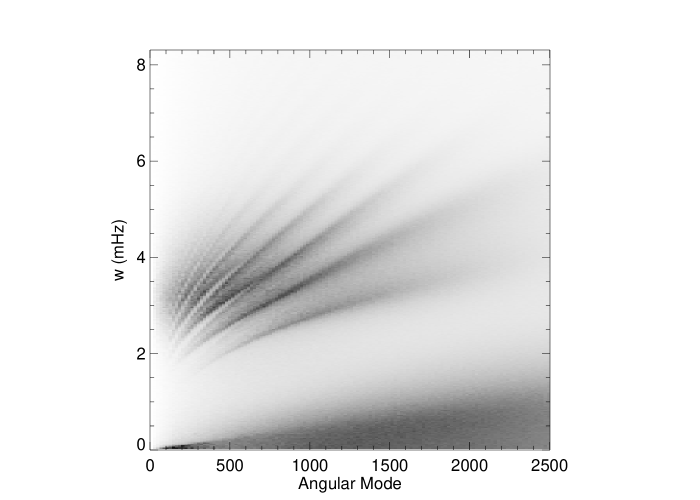
Figure 3: In the left panel, we show the CMB power spectrum as measured by the latest data from the WMAP wmap , BOOMERANG boomerang , VSAvsa , QUADquad , CBI cbi and ACBAR acbar experiments. In the right panel, we show oscillation modes of the solar surface, made using a representative example of SOHO soho MDI data. The prominent ridges correspond to different radial modes, while the low frequency structure is ‘noise’ below the sound speed. The same diagram for the CMB would consist of a single line, $\omega\propto\ell$, but with an extremely small coefficient, so that it would lie almost along the $x$-axis.

III.3 Solar oscillations

In the CMB, the oscillation modes are mainly acoustic in nature. In the Sun the modes are acoustic (‘p-modes’), gravity (‘g-modes’) and surface waves (‘f-modes’). Acoustic oscillations are driven by pressure variations, whereas g-modes are driven by buoyancy of fluid parcels (gravity provides the restoring force). Surface waves arise from discontinuities in density along the surface and propagate along these discontinuities. Neither gravity nor surface waves are possible in the CMB at linear order, due to the isotropy of temperature at zeroth order.

In solar models spherical symmetry and boundary conditions at the surface are enforced. This leads to a set of discrete oscillation frequencies $\omega_{n\ell m}$, where $\ell$ and $m$ are the degree and order of spherical harmonics, and $n$ is the radial node number. These frequencies are independent of $m$ for a spherically symmetric non-rotating star. However, if the star is rotating (as is usually the case), this splits the frequencies, in a similar fashion to the Zeeman or Stark effects for spectral lines. The $+m$ modes travel at a different speed around the star than the $-m$ modes. Thus observations of this splitting over many different multiplets enables reconstruction of the solar interior rotation.

In the Sun the period of acoustic oscillation is dependent on the radial node number $n$. When a helioseismologist talks about the ‘fundamental’, what is meant is the radial mode which has a node at the centre and an anti-node at the surface. The harmonics are then the radial modes with extra numbers of nodes. Each of these radial modes can have a whole set of angular harmonics with different $\ell$ (and $m$). The frequencies can be estimated from the time taken for a sound wave to travel one horizontal wavelength, which gives $\omega\,{\sim}\,c_{\rm s}\ell/R$ (for a wave propagating at depth $R$). The fundamental node ($n=0$) has a period of ${\sim}\,1$ hour, coming approximately from the free-fall time $(G\rho)^{-1/2}$. Typical observed modes have $n=20$–30, with a period of ${\sim}\,5$ minutes. However, there is not really a fundamental angular mode for the Sun in the way that there is for the CMB (although see Section IV).

Since the solar oscillation timescale is much (much!) shorter than the cosmological timescale, helioseismologists have a more powerful signature of acoustics in the Sun than the acoustic peaks frozen onto the CMB – they can observe the actual oscillations and measure their frequencies directly, instead of simply inferring the oscillations from a harmonic imprint. These observations can be captured in an $\ell$–$\nu$ plot, where the angular frequencies are plotted against the temporal frequencies, as shown in Fig. 3. The ridges in this plot correspond to node number – the ridge with lowest temporal frequency corresponds to the fundamental mode. Since modes with small $n$ probe deeper into the solar interior, they can be used to constrain radially dependent properties.

Two key effects in the Sun prevent us from seeing coherent acoustic modes like we observe in the CMB. Firstly the modes are probably generated by turbulent eddies in the convection zone, so that there is stochastic forcing of the oscillations, with random temporal phases. And secondly the very long lifetime of a star compared with its typical mode timescale ($\omega T_{\odot}\,{\sim}\,10^{15}$) ensures that even if initial conditions were synchronized like for the Universe, stochastic excitation would almost immediately lead to loss of coherence.

To summarize, in Table 1 we contrast some of the features of the the Universe with those of the Sun.

The Sun	The Universe
We’re outside, looking in	We’re at the centre!
Solar photosphere	Last scattering surface
${\sim}\,0.1$% thick photosphere	${\sim}\,$10% thick photosphere
Photons made in nuclear core	Photons made in early nuclear processes
Complex scattering	Thomson scattering
Solar spectrum of absorption lines	Weak emission lines of H and He
$T\,{\sim}\,6000\,$K	$T\,{\sim}\,3000\,$K (redshifted)
G dwarf star	M (super-duper) giant star
$R_{\odot}$	$10^{17}R_{\odot}$
Helioseismic modes	CMB anisotropies
Information from mode frequencies	Information from angular power spectrum
Time variations ${\sim}\,5$ minutes	Time variations ${\sim}\,10^{10}$ years
Stochastic, continual excitation	Synchronized initial conditions
Rotation axis defines $m$	No preferred directions

Table 1: Summary of similarities and differences between CMBology and helioseismology.

III.4 Observation and interpretation of oscillations

At present, the instrument which has produced the most sensitive full-sky maps of the CMB is the Wilkinson Microwave Anisotropy Probe (WMAP) wmap . For the Sun, the analogous instrument is the Michelson Doppler Imager (MDI) on board the Solar and Heliospheric Observatory (SOHO) soho .

WMAP measures temperature differences on the sky with an instrument located at the L2 Lagrange point of the Earth-Sun system, which lies about $1.5$ million km on the opposite side of the Earth from the Sun. WMAP has an angular resolution of $0.22^{\circ}$, which means it can measure anisotropies up to $\ell\,{\sim}\,800$.

MDI measures the Doppler shifts of the gas in the solar photosphere on a spacecraft located at the L1 Lagrange point, which lies at the same distance from the Earth as L2, but on the Sun side. MDI has an angular resolution of about $0.0006^{\circ}$ when observing the full solar disk, such that the pixel resolution on the solar surface is around $R_{\odot}/500$. However, since the Sun is not an inside-out star, the origin for the spherical harmonic coordinate system is the solar centre, and this means that MDI can measure anisotropies out to $\ell\,{\sim}\,1000$. This is coincidentally similar to the WMAP resolution.

The solar oscillation spectrum in Fig. 3 was produced using 11 hours of nearly continuous high-resolution MDI solar dopplergrams, consisting of one-minute integrations. Helioseismologists studying such data have access to several years of uninterrupted dopplergrams, but the basic information is evident using this limited data-set.

The information extracted from the modes has a different form for each of the 2 fields we are comparing. In cosmology one makes a CMB map, extracts the power spectrum of anisotropies and typically uses a least-squares routine to fit a cosmological model to the data. It is remarkable that only 6 parameters (within a simple isotropic, homogeneous framework) are needed to provide an excellent fit to WMAP data. In helioseismology, fitting to the acoustic frequencies are often computed using direct inversion techniques on the data. These are then used to tune the solar model, where the ‘parameters’ include some unknown radial functions.

IV A power spectrum of the Sun

CMBologists learn about the Universe from the CMB power spectrum, because it contains almost all the useful information, together with the fact that the linear perturbation theory is remarkably simple. In contrast, the full theory for the amplitudes of helioseismic modes would have to be non-linear, and hence is far from simple. Because of this, the amplitude information of solar modes is often set aside in order to focus on the frequencies.

Nevertheless, we can ask what the mode power spectrum would look like for the Sun, in analogy with the CMB $C_{\ell}$s. In the solar $\ell$–$\nu$ plot (Fig. 3) the ridges are p-modes with different radial mode number, $n$, while the signal at lower temporal frequencies is dominated by convective and other noise effects. This is mainly from convective granulation and supergranulation motions, and although these are interesting in their own right, they will obscure the acoustic oscillations. We therefore remove this low (temporal) frequency signal from the MDI data before attempting to make a power spectrum. We do this by cutting out everything in $\ell$–$\nu$ which would lie below the surface sound speed (following Georgobiani ), which is the lowest speed at which acoustic modes can propagate in the interior.

We can make an order of magnitude conversion to temperature using a blackbody model for the luminosity: $L=4\pi R^{2}\sigma T_{\rm eff}^{4}$, where $\sigma$ is the Stefan-Boltzmann constant. If for simplicity we take $L$ as constant over any oscillation, then $\Delta T/T\,{\simeq}\,V/2\omega R_{\odot}$, where $V$ is an average of the velocity integrated over time, and $\omega$ is the measured oscillation frequency. Performing this scaling to ‘temperature units’, integrating MDI data over all frequencies, and correcting for some instrumental efficiency effects, gives the curve shown in Fig. 4. Remarkably, the CMB power spectrum needs only to be scaled up by about an order of magnitude in order to be comparable. This mean that in terms of $\Delta T/T$ amplitude the two power spectra are within about a factor of three, although of course the shapes of the 2 curves are quite different.

Figure 4: Comparison of CMB and solar power spectra.

IV.1 Conclusions

We have shown interesting analogies between the fields of CMBology and helioseismology. One could contrast more features – for example looking at the polarization information or comparing details of how the Sun and the Universe have changed over time. However, we have probably carried this analogy far enough to be useful in understanding more of the physics of both the CMB and the Sun.

As a final remark, we note that as well as learning about the Sun through its acoustic structure, astrophysicists are also beginning to learn about the interiors of other stars – the science of Asteroseismology. For example, since 2003 the microsatellite MOST most has been studying low angular degree modes in many nearby stars. If there is a further analogy to be drawn here, it may be that each of these stars is like a separate inside-out universe, and Asteroseismology is like studying the multiverse!

References

- (1) See e.g. Scott D., Smoot G.F., 2006, ‘Cosmic Microwave Background Mini-review’, in Yao W.-M., et al., ‘The Review of Particle Physics’, J. Phys. G33, 1 [astro-ph/0601307] and 2007 web update at http://pdg.lbl.gov/
- (2) See e.g. Christensen-Dalsgaard J., 2003, ‘Helioseismology’, Rev. Mod. Phys., 74, 1073–1129 [astro-ph/0207403]
- (3) Further discussion of the physics of CMB acoustic oscillations can be found in: Scott D., White M., 1995, ‘Echoes of Gravity’, Gen. Rel. Grav., 27, 1023–1030 [astro-ph/9505102]; Hu W., Sugiyama N., Silk J., 1997, ‘The Physics of Microwave Background Anisotropies’, Nature, 386, 37–43 [astro-ph/9604166]; Hu W., White, 2004, ‘The Cosmic Symphony’, Sci. American, 290, 44–53. The web-page of Mark Whittle also has some interesting visuals and sound files on ‘Big Bang Acoustics’: http://www.astro.virginia.edu/dmw8f/
- (4) See http://map.gsfc.nasa.gov/
- (5) See http://www.astro.caltech.edu/lgg/boomerang_front.htm
- (6) See http://www.jb.man.ac.uk/research/cmb/vsa/
- (7) See http://www.stanford.edu/schurch/quad.html
- (8) See http://www.astro.caltech.edu/tjp/CBI/
- (9) See http://cosmology.berkeley.edu/group/swlh/acbar/
- (10) See http://sohowww.nascom.nasa.gov/
- (11) D. Georgobiani, J. Zhao and A. .G. Kosovichev, 2007, ‘Local Helioseismology and Correlation Tracking Analysis of Surface Structures in Realistic Simulations of Solar Convection’, Astrophys. J. 657, 1157–1161
- (12) See http://www.astro.ubc.ca/MOST/