Strings in five-dimensional anti-de Sitter space with a symmetry

Abstract

The equation of motion of an extended object in spacetime reduces to an ordinary differential equation in the presence of symmetry. By properly defining of the symmetry with notion of cohomogeneity, we discuss the method for classifying all these extended objects. We carry out the classification for the strings in the five-dimensional anti-de Sitter space by the effective use of the local isomorphism between $\operatorname{{\it SO}}(4,2)$ and $\operatorname{{\it SU}}(2,2)$. We present a general method for solving the trajectory of the Nambu-Goto string and apply to a case obtained by the classification, thereby find a new solution which has properties unique to odd-dimensional anti-de Sitter spaces. The geometry of the solution is analized and found to be a timelike helicoid-like surface.

I Introduction

Existence and dynamics of extended objects play important roles in various stages in cosmology. Examples of extended objects include topological defects, such as strings and membranes, and the Universe as a whole embedded in a higher-dimensional spacetime in the context of the brane-world universe model RanSun99PRL .

The trajectory of an extended object forms a hypersurface in the spacetime which is determined by a partial differential equation (PDE). For example, a test string is described by the Nambu-Goto equation which is a PDE in two dimensions. Because the dynamics is more complicated than that of a particle, one usually cannot obtain general solutions. One way to find exact solutions is to assume symmetry. The simplest solutions to such a PDE are homogeneous ones, in which case the problem reduces to a set of algebraic equations. However, the solutions do not have much variety and the dynamics is trivial.

One may expect that if we assume “less” homogeneity, the equation still remains tractable and the solutions have enough variety to include nontrivial configurations and dynamics of physical interest. The cohomogeneity-one objects give such a class, which helps us to understand the basic properties of the extended objects and serves as a base camp to explore their general dynamics. For a string, stationarity is a special case of the cohomogeneity one condition. Some stationary configurations of the Nambu-Goto strings are obtained in the Schwarzchild spacetime FSZH . Even in the Minkowski space, many nontrivial cohomogeneity-one solutions of the string were recently found ogawa ; IshKoz05PRD . A cohomogeneity-one object is defined, roughly speaking, as the one whose world sheet is homogeneous except in one direction. Then any covariant PDE governing such an object reduces to an ordinary differential equation (ODE), which can easily be solved analytically, or at least, numerically. A solution represents the dynamics of a spatially homogeneous object, or the nontrivial configuration of a stationary object, depending on the homogeneous “direction” is spacelike or timelike. The case of null homogeneous “direction” should also give new intriguing models.

In this paper, we treat strings in the five-dimensional anti-de Sitter space ${AdS}^{5}$. The choice of the spacetime is to meet the recent interest in higher-dimensional cosmology, including the brane-world universe model, and in string theory, though the method developed here is applicable to any background spacetime. A particular example which has recently been attracting much attention is the string in a spacetime with large extra dimensions, which are suggested e.g. by the brane-world model. A detailed investigation Jackson:2004zg suggests that the reconnection probability for this type of strings is significantly suppressed. Then, contrary to what had usually been believed, the strings in the Universe can stay long enough to be considered stationary. Therefore classifying cohomogeneity-one strings and solving dynamics thereof are important for examining the roles of the string in cosmology. We first give the classification of all cohomogeneity-one strings which is valid for any covariant equation of motion. Then, in the case of Nambu-Goto strings, we give a general method for solving the trajectory. The method can be easily applied to the cases of other equations of motion. We demonstrate the procedure and give explicit solutions in some particular cases.

In the classification, we make use of the local isomorphism between $\operatorname{{\it SO}}(4,2)$ and $\operatorname{{\it SU}}(2,2)$ in an essential way. The latter group is easier to treat because the dimensionality of the matrix is lower and because the Jordan decomposition of complex matrices is simpler than that of real ones. Therefore, though a similar classification of Killing fields is found in literature in the context of constructing quotient spaces of the anti-de Sitter space HolPel97CQG , we present an alternative proof based on the classification of $H$-anti-selfadjoint matrices in the Appendix.

In Sec. II, we give a method for the classification of all cohomogeneity-one strings in general, and a method for solving the equations of motions for Nambu-Goto strings. The latter can be easily applied to other equations of motion. In Sec. III, The useful relation of the isometry group ${\operatorname{{\it SO}}(4,2)_{0}}$ and ${\operatorname{{\it SU}}(2,2)}$ is briefly explained. We give the classification of the cohomogeneity-one strings in the anti-de Sitter space in Sec. IV. In Sec. V, we demonstrate the method presented in Sec. II by an example. There we solve the Nambu-Goto equation and examine the geometry of its world sheet. Sec. VI is devoted for conclusion.

In this paper, a spacetime $({\cal M},g)$ is a manifold ${\cal M}$ endowed with a Lorentzian metric $g$. We denote by $G$ the identity component of the isometry group of $({\cal M},g)$, and by ${\mathfrak{g}}$ its Lie algebra. We use the unit such that the speed of light and Newton’s constant are one.

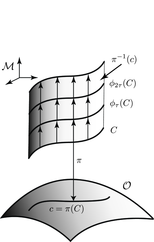
Figure 1: To solve a trajectory of the cohomogeneity-one string is to find a curve $C$ in ${\cal M}$ which projects to a geodesic $c$ on ${\cal O}$.

II General treatment of cohomogeneity-one strings

In this section, we develop a general method for classifying cohomogeneity-one objects and solving their dynamics in an arbitrary spacetime $({\cal M},g)$. Let us start with the definition of the cohomogeneity-one objects. We say that a $m$-dimensional hypersurface ${\cal S}$ in ${\cal M}$ is of cohomogeneity one if it is foliated by $(m-1)$-dimensional submanifolds ${\cal S}_{\sigma}$ labeled by a real number $\sigma$ and there is a subgroup $K$ of $G$ which preserves the foliation and acts transitively on ${\cal S}_{\sigma}$. In particular, the hypersurfaces ${\cal S}_{\sigma}$’s are embedded homogeneously in ${\cal M}$. A cohomogeneity-one object has a world sheet which is a cohomogeneity-one hypersurface. In this paper, we focus on the case that the extended objects are strings, so that $m=2$, and $K$ is a one-parameter group $(\phi_{\tau})_{\tau\in{\mathbb{R}}}$ of isometries.

First, let us consider how to classify the cohomogeneity-one strings. Given a one-dimensional subgroup $K\subset G$ and a point $p\in M$, the equations of motion determines a unique world sheet of a cohomogeneity-one object. The dynamics of the two strings can be considered the same if there is an isometry sending one of their trajectories, ${\cal S}$, to the other, ${\cal S}^{\prime}$. In this paper, we identify the two dynamics if we can do so gradually, namely, if there is a one-parameter group of isometries $(\phi^{\prime}_{\lambda})_{\lambda\in[0,1]}$ such that $\phi^{\prime}_{0}$ is the identity and $\phi^{\prime}_{1}({\cal S})={\cal S}^{\prime}$. We therefore classify the cohomogeneity-one strings up to isometry connected to the identity. In terms of Killing vector fields, it is to classify the Killing vector field $\xi$ generating $K$ up to scalar multiplication and up to isometry. Namely, $\xi$ and $a\phi_{*}\xi$ are equivalent if there exists $\phi\in G$ and $a\neq 0$. To put it more algebraically, the task is to find ${\mathfrak{g}}/\operatorname{Ad}_{G}$ up to scalar multiplication.

Second, let us give a formalism to solve the dynamics and the configuration of the cohomogeneity-one strings. We assume that the string is described by the Nambu-Goto action

$$S=\int_{S}\sqrt{-g_{ab}dx^{a}dx^{b}}.$$

The orbit space of the string with the symmetry group $K$ is defined by ${\cal O}:={\cal M}/K$, i.e., by identifying all the points on each Killing orbit in ${\cal M}$. The submanifolds ${\cal S}_{\sigma}$ mentioned above are the preimages $\pi^{-1}(x)$ of a point $x\in{\cal O}$. One can endow ${\cal O}$ with a metric $h$ so that the projection $\pi:({\cal M},g)\to({\cal O},h)$ is an orthogonal projection, or more precisely, a Riemannian submersion. The metric $h$ is given by

$$h_{ab}:=g_{ab}-\xi_{a}\xi_{b}/f,$$ (1)

where $f:=\xi^{a}\xi_{a}$. This metric has the Euclidean signature if the Killing vector $\xi$ is timelike, i.e., if $f<0$, and the Lorentzian signature if $\xi$ is spacelike, i.e., if $f>0$. Carrying out the integration along $\xi$ in the Nambu-Goto action, one obtains

$$S=\int_{c}\sqrt{-fh_{ab}dx^{a}dx^{b}},$$ (2)

where $c$ is a curve on ${{\cal O}}$. Thus the problem of the string reduces to finding geodesics on the orbit space ${\cal O}$ with the metric $-fh$. For convenience, we adopt a modified action

$$S=\int_{c}d\sigma{\left(-\frac{1}{\alpha}fh_{ab}\dot{x}^{a}\dot{x}^{b}+{\alpha}\right)},$$ (3)

where an overdot denotes the differentiation by $\sigma$. The action 3 derives the same geodesic equations as 2 and retains the invariance under reparametrization of $\sigma$. The function ${\alpha}$ is the norm of the tangent vector.

The two-dimensional world sheet of the string is the preimage $\pi^{-1}(c)$ of the geodesic $c$ on $({\cal O},-fh)$. However, it is sometimes more convenient to find a lift curve ${C}$ on ${\cal M}$ whose projection $\pi({C})$ is a geodesic on $({\cal O},-fh)$ than to find a geodesic on $({\cal O},-fh)$ (Fig. 1). The Hopf string in Sec. V is such an example. In the case, the trajectory of the string is given by

$${\cal S} =\pi^{-1}(\pi({C}))$$

$$=\{\phi_{\tau}({C}(\sigma));\,(\tau,\sigma)\in{\mathbb{R}}^{2}\}.$$ (4)

Note that the last expression in 4 depends on the objects in ${\cal M}$ only. Thus the trajectory ${\cal S}$ can be viewed as a foliation by mutually isometric curves $\phi_{\tau}\circ{C}$ labeled by $\tau$.

After one obtains the solutions of the equation of motion, one may want to classify their trajectories up to isometry. This can be done by identifying $C$ (or ${\cal S}$) which are related by homogeneity-preserving isometries. We say that an isometry $\Phi$ is homogeneity-preserving if it preserves the action of $K$, i.e., if it satisfies

$$\Phi\circ K\circ\Phi^{-1}=K.$$ (5)

The homogeneity-preserving isometries form a group. In algebraic terms, the group is the normalizer of $K$ in the group $G$ of isometries on ${\cal M}$, which is denoted by $N_{G}(K)$. Its Lie algebra is the idealizer of ${{\mathfrak{k}}}$ in ${{\mathfrak{g}}}$ which is denoted by $N_{{\mathfrak{g}}}({\mathfrak{k}})$.

We note that in the special case that $\Phi$ commutes with the action of $K$, i.e. when $\Phi$ is in the centralizer $Z_{G}(K)$ of $K$ in $G$, the squared norm of $\xi$ must be invariant under $\Phi$. This can be seen from $\Phi_{*}f=\Phi_{*}(g_{ab}\xi^{a}\xi^{b})=(\Phi_{*}g_{ab})\xi^{a}\xi^{b}+g_{ab}(\Phi_{*}\xi^{a})\xi^{b}+g_{ab}\xi^{a}(\Phi_{*}\xi^{b})=f$, where we have used $\Phi_{*}g_{ab}=g_{ab}$ and $\Phi_{*}\xi^{a}=\xi^{a}$.

The whole procedure of solving the dynamics is explicitly carried out for an example in Sec. V.

III ${AdS}^{5}$ and its isometry group

Hereafter in this paper, we assume that the spacetime $({\cal M},g)$ is the five-dimensional anti-de Sitter space ${AdS}^{5}$, or its universal cover $\widetilde{{AdS}^{5}}$. The former space has closed timelike curves which in the latter space are “opened up” to infinite nonclosed curves. The latter is usually more suitable when we discuss cosmology, but we will not distinguish them strictly in the following.

The space ${AdS}^{5}$ is the most easily expressed as a pseudo-sphere

$$\overline{\psi}{\psi}=-1$$ (6)

in the pseudo-Euclidean space $E^{4,2}$ whose metric is $dS^{2}=l^{2}d\overline{\psi}d{\psi}$, where we have used complex coordinates ${\psi}:=({\psi}^{0},{\psi}^{1},{\psi}^{2})^{T}\in{\mathbb{C}}^{3}$, and have defined $\overline{\psi}:={\psi}^{\dagger}\zeta$ and $\zeta:={\mbox{\rm diag}}[-1,1,1]$.

The isometry group of ${AdS}^{5}$ is ${\operatorname{{\it SO}}(4,2)}$ acting on $(s,t,x,y,z,w)^{T}\in{\mathbb{R}}^{6}$, where ${\psi}^{0}:=s+it$, ${\psi}^{1}:=x+iy$, and ${\psi}^{2}:=z+iw$. In the classification of the strings, however, we take advantage of the isomorphism ${\operatorname{{\it SO}}(4,2)_{0}}\simeq{\operatorname{{\it SU}}(2,2)}/\{\pm 1\}$ and work with ${\operatorname{{\it SU}}(2,2)}$. Let $V$ be the vector space whose elements are complex symmetric matrices of the form

$$p =\begin{bmatrix}0&({\psi}^{0})^{*}&-{\psi}^{2}&({\psi}^{1})^{*}\\ ({\psi}^{0})^{*}&0&{\psi}^{2}&({\psi}^{2})^{*}\\ {\psi}^{2}&-{\psi}^{1}&0&{\psi}^{0}\\ -({\psi}^{1})^{*}&-({\psi}^{2})^{*}&{\psi}^{0}&0\end{bmatrix}$$

$$=si\sigma_{z}\otimes\sigma_{y}+t1\otimes\sigma_{y}+xi\sigma_{y}\otimes\sigma_{z}$$

$$\qquad+y\sigma_{x}\otimes 1-zi\sigma_{y}\otimes\sigma_{x}+w\sigma_{x}\otimes\sigma_{y},$$ (7)

where $\sigma_{x}$, $\sigma_{y}$ and $\sigma_{z}$ are the Pauli matrices and $1$ is the $2\times 2$ identity matrix. The action of an element of ${\operatorname{{\it SO}}(4,2)_{0}}$ on $E^{4,2}$ corresponds to the action of $U\in{\operatorname{{\it SU}}(2,2)}$ on $V$ in the following way (Yok90, , p106):

$$p\mapsto UpU^{T}.$$ (8)

The Lie algebra ${{\mathfrak{s}}{\mathfrak{u}}(2,2)}$ of ${\operatorname{{\it SU}}(2,2)}$ consists of the matrices $X=$ satisfying $X\eta+\eta X^{\dagger}=0$, where ${\eta}:={\mbox{\rm diag}}[1,1,-1,-1]$. The explicit form is

$$X=\left[\begin{array}[]{cc}{\beta}&{\gamma}\\ {\gamma^{\dagger}}&{\delta}\end{array}\right],$$ (11)

where $\gamma$ is a $2\times 2$ complex matrix, and $\beta$ and $\delta$ are $2\times 2$ anti-Hermitian matrices. The infinitesimal transformation for 8 is given by the action of $X\in{{\mathfrak{s}}{\mathfrak{u}}(2,2)}$ as

$$p\mapsto Xp+pX^{T}=\{X_{S},p\}+[X_{A},p],$$ (12)

where $X_{S}:=(X+X^{T})/2$ and $X_{A}:=(X-X^{T})/2$ are the symmetric and antisimmetric parts, respectively, of $X$. The correspondence between the ${{\mathfrak{s}}{\mathfrak{u}}(2,2)}$ and ${{\mathfrak{s}}{\mathfrak{o}}(4,2)}$ infinitesimal transformations are given in Table 1, where $X=(e_{1}\otimes e_{2})/2$. In the table, $J_{xy}$ denotes the rotation in the $xy$ plane, $L$ denotes the rotation in the $st$ plane, $K_{x}$ denotes the $t$-boost in the $x$ direction, $\widetilde{K}_{w}$ denotes the $s$-boost in the $w$ direction, etc.

	1	$\sigma_{x}$	$\sigma_{y}$	$\sigma_{z}$
$1/i$		$J_{yz}$	$J_{zx}$	$J_{xy}$
$\sigma_{x}$	$K_{w}$	$\widetilde{K}_{x}$	$\widetilde{K}_{y}$	$\widetilde{K}_{z}$
$\sigma_{y}$	$-\widetilde{K}_{w}$	$K_{x}$	$K_{y}$	$K_{z}$
$\sigma_{z}/i$	$L$	$J_{wx}$	$J_{wy}$	$J_{wz}$

Table 1: Correspondence between the ${{\mathfrak{s}}{\mathfrak{u}}(2,2)}$ and ${{\mathfrak{s}}{\mathfrak{o}}(4,2)}$ transformations.

IV The classification

In this section, we obtain the classification of the cohomogeneity-one strings in ${AdS}^{5}$. As discussed in Sec. II, the classification is to find ${\mathfrak{g}}/\operatorname{Ad}_{G}$ up to scalar multiplication, where $G={\operatorname{{\it SO}}(4,2)_{0}}$. Because ${\operatorname{{\it SO}}(4,2)_{0}}$ is isomorphic to ${\operatorname{{\it SU}}(2,2)}/\{\pm 1\}$ as is seen in Sec. III, ${{\mathfrak{s}}{\mathfrak{o}}(4,2)}/\operatorname{Ad}_{\operatorname{{\it SO}}(4,2)_{0}}$ is isomorphic to ${{\mathfrak{s}}{\mathfrak{u}}(2,2)}/\operatorname{Ad}_{\operatorname{{\it SU}}(2,2)}$. Thus the classification is to find ${{\mathfrak{s}}{\mathfrak{u}}(2,2)}/\operatorname{Ad}_{\operatorname{{\it SU}}(2,2)}$ up to scalar multiplication. However, the equivalence classes ${{\mathfrak{s}}{\mathfrak{u}}(2,2)}/\operatorname{Ad}_{\operatorname{{\it SU}}(2,2)}$ is known as in the Lemma below, so that we can easily classify the cohomogeneity-one strings by further identifying the equivalence classes by scalar multiplications.

We begin with introducing some terms which is necessary to state the Lemma. Let $H$ be an invertible Hermitian matrix. The $H$-adjoint of a square matrix $A$ is defined by ${A}^{\star}:=H^{-1}A^{\dagger}H$. A matrix $A$ is called $H$-selfadjoint when ${A}^{\star}=A$, $H$-anti-selfadjoint when ${A}^{\star}=-A$, and $H$-unitary when $A{A}^{\star}={A}^{\star}A=1$. We say that matrices $A$ and $B$ are $H$-unitarily similar and write $A\stackrel{{\scriptstyle H}}{{\sim}}B$ if there exists an $H$-unitary matrix $W$ satisfying $B=WAW^{-1}$. In these terms, ${\operatorname{{\it SU}}(2,2)}$ is the group of unimodular ${\eta}$-unitary matrices and ${{\mathfrak{s}}{\mathfrak{u}}(2,2)}$ is the Lie algebra of traceless ${\eta}$-anti-selfadjoint matrices. Thus, from the discussion in Sec. II, our task of classifying cohomogeneity-one strings is to classify the elements of ${{\mathfrak{s}}{\mathfrak{u}}(2,2)}$ up to equivalence relation $\stackrel{{\scriptstyle\rm\eta}}{{\sim}}$ and up to scalar multiplication.

Let us introduce another equivalence relation closely related to the one above. Let $(A,H)$ be a pair of a complex matrix and an invertible Hermitian matrix $H$. The pairs $(A,H)$ and $(A^{\prime},H^{\prime})$ are said unitarily similar if there is a complex matrix $W$ such that $A^{\prime}=WAW^{-1},H^{\prime}=WHW^{\dagger}$ GLR83 . This is an equivalence relation and will be denoted by $(A,H)\sim(A^{\prime},H^{\prime})$. Note that $A\stackrel{{\scriptstyle\rm\eta}}{{\sim}}A^{\prime}$ is equivalent to $(A,{\eta})\sim(A^{\prime},{\eta})$. Let $A$ be an $H$-selfadjoint matrix. Then if $\lambda$ is an eigenvalue of $A$, so is its complex conjugate $\lambda^{*}$. Let $J_{0}(\lambda)$ be the Jordan block with eigenvalue $\lambda$ and let

$$J(\lambda):=\begin{cases}J_{0}(\lambda),&\text{$\lambda$ is real},\\ {\mbox{\rm diag}}[J_{0}(\lambda),J_{0}(\lambda^{*})],&\text{$\lambda$ is non-real}.\end{cases}$$ (13)

Now we can state the Lemma GLR83 .

Lemma.

If $A$ is $H$-selfadjoint, then $(A,H)\sim(J,P)$ with

$$J ={\mbox{\rm diag}}{\left[J(\lambda_{1}),\ldots,J(\lambda_{\beta})\right]},$$ (14)

$$P ={\mbox{\rm diag}}{\left[{\epsilon}_{1}P_{1},\ldots,{\epsilon}_{\alpha}P_{\alpha},P_{\alpha+1},\ldots,P_{\beta}\right]},$$

$${\epsilon}_{j} =\pm 1,\quad P_{j}={\tiny\begin{bmatrix}{0}&{}&1\\ {}&{\mathinner{\mkern 1.0mu\raise 1.0pt\hbox{.}\mkern 2.0mu\raise 4.0pt\hbox{.}\mkern 2.0mu\raise 7.0pt\vbox{\kern 7.0pt\hbox{.}}\mkern 1.0mu}}&{}\\ 1&{}&{\large 0}\end{bmatrix}},$$ (15)

where $\lambda_{1},\ldots,\lambda_{\alpha}$ are the real eigenvalues of $A$, $\lambda_{\alpha+1},\lambda_{\alpha+1}^{*},\ldots,\lambda_{\beta},\lambda_{\beta}^{*}$ are the non-real eigenvalues of $A$, and the size of $P_{j}$ is the same as that of $J(\lambda_{j})$.

For any $X\in{{\mathfrak{s}}{\mathfrak{u}}(2,2)}$, there is a pair $(J,P)$ in the Lemma such that $(X/i,\eta)\sim(J,P)$, because $X/i$ is ${\eta}$-selfadjoint. We will denote the type of $X$ by

$$\text{\rm Type}(X):=({\epsilon}_{1}d_{1},\ldots{\epsilon}_{\alpha}d_{\alpha}|d_{\alpha+1}/2,\ldots,d_{\beta}/2),$$ (16)

where $d_{j}:=\dim J(\lambda_{j})$. [If there is either no real ($\alpha=0$) or no non-real ($\alpha=4$) eigenvalues, we put a 0 in the corresnponding slot.] We combine all the types with the same $d_{j}$ and call it the (major) type $[d_{1},\ldots d_{\alpha}|d_{\alpha+1}/2,\ldots,d_{\beta}/2]$, and we call $({\epsilon}_{1},\cdots,{\epsilon}_{\alpha})$ the minor type. In the Theorem below, $J_{xy}$ denotes spatial rotations in the $xy$ plane, $K_{z}$ denotes the boost with respect to the time $t$ in the $z$ direction, $\widetilde{K}_{w}$ denotes the boost with respect to the time $s$ in the $w$ direction, $L$ denotes the rotation in the $st$ plane, etc.

Type	Killing vector field $\xi$
$(4|0)$	$\displaystyle{K_{x}+\widetilde{K}_{y}+J_{xy}+L}+2(J_{yz}+K_{z})$
$\pm(3,1|0)$	$\displaystyle K_{x}+\widetilde{K}_{y}+J_{yz}\pm J_{xw}+a(J_{xy}-L\mp J_{zw})$
$(2,2|0)$	$K_{x}+L+aJ_{yz}$
$(2,-2|0)$	$K_{x}+J_{xy}+aJ_{zw}$
$(2,1,1|0)$	$K_{x}+\widetilde{K}_{y}+J_{xy}+L+a\,J_{zw}+b\,(J_{xy}-L)$
$(1,1,1,1|0)$	$a\,L+b\,J_{xy}+c\,J_{zw}$ ($a^{2}+b^{2}+c^{2}=1$)
$(2|1)$	$K_{x}+\widetilde{K}_{y}+L+J_{xy}+aJ_{zw}+b(K_{y}+\widetilde{K}_{x})$
$(1,1|1)$	$K_{x}+\widetilde{K}_{y}+b\,(L-J_{xy})+c\,J_{zw}$
$(0|2)$	$K_{x}+J_{xy}+a\,\widetilde{K}_{z}$ ($a\neq 0$)
$(0|1,1)$	$aK_{x}+b\,\widetilde{K}_{y}+c\,J_{zw}\quad(b\neq\pm a,\ a^{2}+b^{2}+c^{2}=1)$

Table 2: The classification of cohomogeneity-one strings. The types of the generator of ${\operatorname{{\it SU}}(2,2)}$ and the corresponding Killing vector fields $\xi$ on ${AdS}^{5}$.

Theorem.

Any one-dimensional connected Lie group of isometries of ${AdS}^{5}$ is generated by one of the nine types of $\xi$ in Table 2 up to isometry of ${AdS}^{5}$ connected to the identity, where $a,b,c$ are real numbers, and the double-signs must be taken in the same order in each expression.

The proof is given in the Appendix. Note in Table 2 that Type $(0|1,1)$ would become Type $(1,1,|1)$ (with $b=0$) if one set $b=\pm a$ and that Type $(0|2)$ would become Type $(2,-2|0)$ (with $a=0$) if one set $a=0$.

V The Hopf string

In this section, we choose a type from the classified strings in the Theorem and find its trajectory. We assume that the string obeys the Nambu-Goto equation and apply the general procedure presented in Sec. II. The example also shows that working with the lift curves as explained in Sec. II can make the calculations and geometric interpretation of the trajectory simple and transparent.

We shall say that a Hopf string is a cohomogeneity-one string which is homogeneous under the change of the overall phase in the complex coordinates $\psi$ defined in Sec. III:

$${\psi}\mapsto e^{i\tau}{\psi},\quad\tau\in{\mathbb{R}}.$$ (17)

This isometry is the simultaneous rotations in the $st$, $xy$, and $zw$ planes. The Killing vector field $\xi$ is proportional to $L+J_{xy}+J_{zw}$ and falls into Type $(1,1,1,1|0)$ with the condition $a=b=c$. The Killing orbits are closed timelike curves in ${AdS}^{5}$. In the universal cover $\widetilde{{AdS}^{5}}$, they are not closed and the string solution represents a stationary string.

Let us find the configurations of the Hopf string by solving the action principle 3 and finding the geodesics on $({\cal O},-fh)$. We first see that the orbit space $({\cal O},h)$ is a Riemannian manifold, since $\xi$ is timelike. Then, from the fact that $f=\xi^{a}\xi_{a}$ is a constant (which we set $-1$), we find that solving the geodesics on $({\cal O},-fh)$ is nothing but solving geodesics on $({\cal O},h)$. One could either introduce some coordinate system on ${\cal O}$ to solve 3 directly or make an ansatz with some coordinate system on ${AdS}^{5}$ to solve 2. Both methods work well but would lead to somewhat complicated equations. In what follows, we would take the advantage of the symmetry, especially the complex structure, of $E^{4,2}$ and find the lift curves on the spacetime ${AdS}^{5}$ which project to the geodesics on $({\cal O},-fh)$, as was explained in Sec. II.

The metric $h$ in 1 for the Hopf string is the usual flat metric $d\overline{\psi}d\psi$ with the contribution from the phase change being subtracted. With the constraint 6, $h$ can be written as

$$h=l^{2}d\overline{\psi}(1-P)d{\psi},$$ (18)

where $P:=-{\psi}\overline{\psi}$ is the normal projection along ${\psi}$. This is the same as the Fubini-Study metric on a projective space ${\mathbb{C}}P^{2}$ except that we started with an indefinite scalar product $\zeta={\mbox{\rm diag}}[-1,1,1]$ in 6 and in $dS^{2}=l^{2}d\overline{\psi}d\psi$, while the usual Fubini-Study metric is defined by means of a positive definite scalar product. We shall also call $h$ as the Fubini-Study metric here and shall denote the Riemannian manifold $({\cal O},h)$ by ${\mathbb{C}}P_{-}^{2}$. The fibration ${\mathbb{C}}P_{-}^{2}\simeq{AdS}^{5}/U(1)$ is the generalization of the Hopf fibration to the case of indefinite scalar product fn-a . Thus the problem of finding Nambu-Goto strings has reduced to solving geodesics on ${\mathbb{C}}P_{-}^{2}$.

Our action 3 for the Hopf string becomes

$$S=\int_{C}d\sigma{\left(\frac{1}{\alpha}\dot{\overline{\psi}}(1+{\psi}\overline{\psi})\dot{{\psi}}+{\alpha}+\mu(1+\overline{\psi}{\psi})\right)},$$ (19)

where $\mu$ is a Lagrange multiplier. This is the action for geodesics on ${\cal O}$ written in terms of the coordinates $\psi$ in $E^{4,2}$. The action 19 has a $U(1)$ gauge invariance ${\psi}(\sigma)\mapsto e^{i\theta(\sigma)}{\psi}(\sigma)$ fn-c which corresponds to the freedom in the choice of a lift. This gauge degree of freedom is used to simplify the calculation. In particular, we shall show that each geodesic on ${\cal O}$ for the Hopf string can always be written in a proper gauge as the projection of a geodesic on ${AdS}^{5}$.

The Euler-Lagrange equations are the constraint 6 and

$$\dot{\overline{\psi}}(1+{\psi}\overline{\psi})\dot{{\psi}}={\alpha}^{2},\qquad$$ (20)

$$-{\left(\frac{1}{\alpha}(1+{\psi}\overline{\psi})\dot{\psi}\right)}\parbox[c][17.22217pt]{10.00002pt}{}^{\bullet}+\frac{1}{\alpha}\dot{\overline{\psi}}\psi\dot{\psi}+\mu{\psi} =0.$$ (21)

Multiplying $\overline{\psi}$ on 21 from the left and using the constraint 6, one obtains an equation which merely determines $\mu$. On the other hand, the time derivative of 6 implies that $\overline{\psi}\dot{\psi}$ is pure imaginary. This value can be changed by the gauge transformation ${\psi}\mapsto e^{i\theta(\sigma)}{\psi}(\sigma)$. We can always choose the gauge ${\rm Re}\overline{\psi}\dot{\psi}=0$ which under the constraint 6 implies

$$\overline{\psi}\dot{\psi}=0.$$ (22)

Geometrically, 22 means that the curve ${C}$ on ${\cal M}$ is horizontal, namely, it is orthogonal, with respect to $g$, to the fiber $\pi^{-1}(\pi\circ{C}(\sigma))$ at each point on ${C}$. Multiplying $1+{\psi}\overline{\psi}$ on 21 from the left, and using 6 and 22, one obtains the geodesic equation for the Fubini-Study metric,

$$(1+{\psi}\overline{\psi}){\left(\frac{\dot{\psi}}{\alpha}\right)}\parbox[c][17.22217pt]{10.00002pt}{}^{\bullet}=0.$$ (23)

Choosing the parameter of the curve to be the proper length so that ${\alpha}\equiv 1$, one can write 23 in a particularly simple form. Since 20 and 22 imply $\overline{\psi}\ddot{\psi}=-\dot{\overline{\psi}}\dot{\psi}=-1$, 23 yields

$$\ddot{\psi}={\psi}.$$ (24)

One can immediately solve the equation to obtain

$${\psi}(\sigma)=A\cosh\sigma+B\sinh\sigma,$$ (25)

$$\overline{A}A=-1,\quad\overline{A}B=0,\quad\overline{B}B=1,$$ (26)

where $A,B\in{\mathbb{C}}^{3}$. The projection $\pi\circ{C}$ of the curves ${C}:\sigma\mapsto\psi(\sigma)$ expressed by 25 are geodesics on ${\cal O}$.

Some remarks are in order. First, the geodesics on the four-dimensional manifold ${\cal O}$ should contain seven independent real constants: the initial position and the direction of the initial velocity. One sees that $\pi\circ{C}$ actually contains seven independent real constants since we have twelve real constants, four constraints 26 and one redundancy, i.e., the phase of $\psi(0)$. Second, the lift curve 25 is a horizontal geodesic on ${AdS}^{5}$. A special feature of the Hopf string is that one can always choose a lift curve $C$—the horizontal lift in this case— of a geodesic $c$ on the orbit space $({\cal O},-fh)$ so that $C$ is also a geodesic on $({\cal M},g)$. Third, a horizontal geodesic ${C}$ on ${AdS}^{5}$ is the intersection of ${AdS}^{5}$ and a two-dimensional plane through the origin in $E^{4,2}$, which corresponds to the great circle in the case of positive definite metric. Thus the hyperbolic curve 25 is unique up to isometry, for any choice of $A$ and $B$. Furthermore, ${C}$ is a Killing orbit on ${AdS}^{5}$.

Now the world sheet ${\cal S}$ of the Hopf string can be written down easily. From 4, 17 and 25, we have

$$\psi(\tau,\sigma)=e^{i\tau}{\left(A\cosh\sigma+B\sinh\sigma\right)},$$ (27)

where $A$ and $B$ satisfy the condition 26.

To describe geometry of the world sheet ${\cal S}$ in more detail, let us introduce a new time coordinate $T$ on ${AdS}^{5}$ defined by

$$T=\arg\psi^{0}=\arg(s+it).$$ (28)

In $\widetilde{{AdS}^{5}}$, $T$ runs from $-\infty$ to $\infty$. The $T=\rm constant$ hypersurfaces embedded in $\widetilde{{AdS}^{5}}$ are Cauchy surfaces. The Killing field $\xi=d/d\tau$ drives the simultaneous rotations in the $xy$ and $zw$ planes while going up along the $T$ axis. Thus the world sheet of the Hopf string can be viewed pictorially as the surface swept by a boomerang 25 flying up while rotating (Fig. 2).

Let us reduce the degrees of freedom of $A$ and $B$ in 25 by the homogeneity-preserving isometries and canonicalize them, as was explained in Sec. II. The Lie algebra $N_{{\mathfrak{g}}}({\mathfrak{k}})$ of the homogeneity-preserving isometries is the vector space spanned by

$$\xi,\;L-J_{xy},\;L+J_{wz},\;J_{yz}+J_{wx},\;J_{zx}+J_{wy},\;$$

$$\widetilde{K}_{z}+K_{w},\;K_{z}-\widetilde{K}_{w},\;\widetilde{K}_{x}+K_{y},\;K_{x}-\widetilde{K}_{y}.$$ (29)

In fact, all generators 29 commutes with $\xi$. The isometries generated by 29 map the solution 27 to another isometric one. First, using the isometries generated by $L$, $J_{xy}$ and $J_{wz}$, one can make a general $A\in{\mathbb{C}}^{3}$ in 26 to be real, i.e., to have no $t$, $y$, $w$ components. Then, by using $\widetilde{K}_{z}+K_{w}$ and $\widetilde{K}_{x}+K_{y}$, one has $A=(1,0,0)^{T}$. Next, we canonicalize $B$ by the isometries which leaves this $A$ unchanged. By $\overline{A}B=0$, $B$ must have the form $B=(0,B^{1},B^{2})$. By using $J_{xy}$ and $J_{wz}$, one can make $B^{1}$ and $B^{2}$ real. Finally, by using $J_{zx}+J_{wy}$, one has $B=(0,1,0)^{T}$, where $\alpha\in{\mathbb{R}}$. As a result, the trajectory 27 can be written up to isometry as

$$\begin{pmatrix}T\\ x\\ y\\ z\\ w\end{pmatrix}=\begin{pmatrix}{\tau}\\ {\sinh\sigma\cos\tau}\\ {\sinh\sigma\sin\tau}\\ 0\\ 0\end{pmatrix},$$ (30)

where we have used $T=\arg(s+it)$. In particular, the world sheet has no parameter and is unique. We can therefore say that the Hopf string has rigidity.

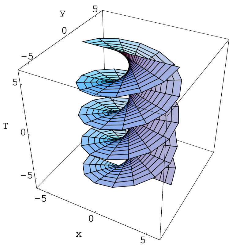
Figure 2: The world sheet of the Hopf string in the case in the coordinates $(T,x,y)$. The other coordinates $z$ and $w$ vanish.

Fig. 2 shows the worls sheet of the Hopf string. This is a helicoid swept by a rotating rod passing through the $T$ axis. This surface is periodic in $T$ direction with period $\pi$. The similar helical motion of an infinite curve in the Minkowski space has a cylinder outside of which the trajectory becomes tachyonic (spacelike). In the anti-de Sitter case, however, the trajectory is always timelike because the physical time passing with the unit difference in $T$ becomes large when the curve is far from the $T$ axis in Fig. 2.

Let us summarize some special features of the Hopf string. (i) The Killing vector $\xi$ has a constant squared norm. (ii) The orbit space $({\cal O},-fh)$ for Nambu-Goto Hopf string inherits the complex structure of $E^{4,2}$, over which ${AdS}^{5}$ admits a Hopf fibration. (iii) The orbit space $({\cal O},-fh)$ is homogeneous and is highly symmetric. (iv) The world sheet of the string is homogeneously embedded and is flat intrinsically. (v) The world sheet of the string is rigid, i.e., it is unique up to isometry.

Among anti-de Sitter spaces, a Killing field satisfying (i) or (ii) exists only in the odd-dimensional ones. In the case of ${AdS}^{5}$, the only Killing vector satisfying (i) is $L+J_{xy}\pm J_{zw}$ up to scaling and rotation of the spatial axes fn-b .

The condition (i) is partially a reason for (ii) and (iii). In the case of the Hopf string, the homogeneity-preserving isometry group $N_{G}(K)$ equals the centralizer $Z_{G}(K)$. On the other hand, $Z_{G}(K)$ must preserve $f$ (Sec. II). Thus (i) in general suggests high symmetry of $({\cal O},-fh)$. In the case of Hopf string, the isometry group of the orbit space is an eight-dimensional group. In fact, The vector fields 29 except the first one $\xi$ form a closed Lie algebra and act on $({\cal O},-fh)$ as Killing fields.

As for (iv), one finds that the resulting world sheet 30 for the Hopf string is invariant under the infinitesimal isometry $\widetilde{K}_{x}+K_{y}$ of ${AdS}^{5}$. Since $\xi$ and $\widetilde{K}_{x}+K_{y}$ commute, the world sheet ${\cal S}$ is acted by ${\mathbb{R}}^{2}$ and is homogeneous. This implies that ${\cal S}$ is flat intrinsically, namely, ${\cal S}$ is the two-dimensional Minkowski space embedded in ${AdS}^{5}$. This can also be verified by a direct computation of the intrinsic metric.

The high symmetry (iii) implies (v) for the Hopf string. Incidentally, stationary strings in ${AdS}^{4}$ ads4 does not have rigidity. They would most naturally correspond in ${AdS}^{5}$ to the cases $\xi\propto L+bJ_{xy}$, which are in the same Type $(1,1,1,1|0)$ as the Hopf string but with different parameters.

These suggest that the Hopf string is similar to the string with simple time translation invariance in the Minkowski space. The Hopf string is the only solution in ${AdS}^{5}$ which shares all of the properties (i), (iii), (iv) and (v) with the flat string in the Minkowski space.

VI Conclusion

The cohomogeneity-one symmetry reduces the partial differential equation governing the dynamics of an extended object in the spacetime ${\cal M}$ to an ordinary differential equation. With applications in higher-dimensional cosmology in mind, we have presented the procedure to classify all cohomogeneity-one strings and solve their trajectories with a given equation of motion. The former is to classify the Killing vector fields up to isometry, and the latter is to solve geodesics on the orbit space $({\cal O},-fh)$ which is the quotient space of ${\cal M}$ by the symmetry group $K$. We have carried out the classification in the case that the spacetime is the five-dimensional anti-de Sitter space, by an effective use of the local isomorphism of $\operatorname{{\it SO}}(4,2)$ and $\operatorname{{\it SU}}(2,2)$ and of the notion of $H$-similarity. Assuming that the string obeys the Nambu-Goto equation, we have solved the world sheet of one of the strings, which we call the Hopf string, in the classification. The problem has reduced to find geodesics on the orbit space $({\cal O},h)$. By using a technique similar to the one used in quntum information theory and working on the lift curves in ${\cal M}$, we have obtained a new solution which describes the trajectories of the Hopf string. They are timelike helicoid-like surfaces around the time axis which is unique up to isometry of ${AdS}^{5}$.

We can say that the Hopf string is the simplest example of string in the anti-de Sitter space which corresponds to a straight static string in the Minkowski space. The Killing vector field defining the symmetry of the string is homogeneous in the spacetime and has a constant norm. This greatly simplifies solving the geodesics on the orbit space and the world sheet becomes homogeneous and rigid, as we have seen in Sec. V. The simplicity of the Hopf strings suggests that they were common in the Universe and played significant roles, if the Universe is higher-dimensional or is a brane-world.

We would like to remark that although we now have all types where the equations of motion reduce to ordinary differential equations this does not in general imply solvability. The solvability problem is nontrivial and strongly related to the structure of the orbit spaces. A systematic analysis will be presented in a future work.

Finally, we would like to remark that the classification presented here will be the basis for that of higher-dimensional cohomogeneity-one objects. The procedure is the following: (i) for each of the Killing vector field $\xi$ classified in Table 2, enumerate how one can add new independent Killing vector fields $\xi^{(1)}$, …, $\xi^{(n)}$ such that $\xi$, $\xi^{(1)}$ …, $\xi^{(n)}$ form a closed Lie algebra ${\mathfrak{k}}^{\prime}$; (ii) reduce the degrees of freedom of ${\mathfrak{k}}^{\prime}$ by using the isometries which preserve $\xi$, thus classifying the Lie algebras ${\mathfrak{k}}^{\prime}$; (iii) examine the orbits in the spacetime generated by ${\mathfrak{k}}^{\prime}$.

Appendix: Proof of the Theorem

Let $X$ be an ${\eta}$-anti-selfadjoint matrix $X$. The Lemma implies that $(X/i,{\eta})\sim(J,P)$ with some $(J,P)$. On the other hand, if ${\eta}=WPW^{\dagger}$, the definition of unitary similarity implies $(J,P)\sim(WJW^{-1},{\eta})$. Thus $(X/i,{\eta})\sim(WJW^{-1},{\eta})$ so that $X\stackrel{{\scriptstyle\rm\eta}}{{\sim}}iWJW^{-1}$. We therefore can carry out the classification by the following procedure: (i) enumerate $(J,P)$ in the Lemma such that there exists $W$ satisfying ${\eta}=WPW^{\dagger}$, (ii) construct $X_{0}=iWJW^{-1}$, (iii) translate $X_{0}$ back to the Killing vector field $\xi$ in ${\operatorname{{\it SO}}(4,2)_{0}}$ by Table 1.

In some cases, however, the canonical pairs $(J,P)$ and $(J^{\prime},P^{\prime})$ correspond to $X_{0}$’s which generate an identical Lie group. This happens when $(J^{\prime},P^{\prime})\sim(\alpha J,P)$ with a nonzero real number $\alpha$. Thus it is important to know how a pair $(\alpha J_{j}(\lambda_{j}),P_{j})$ can be canonicalized. For $\alpha>0$, we simply have $(\alpha J_{j}(\lambda_{j}),P_{j})\sim(J_{j}(\alpha\lambda_{j}),P_{j})$, so that they generate an identical group. Thus we focus on $(-J_{j}(\lambda_{j}),P_{j})$ in the following. When $d_{j}$ is odd, we have

$$(-J(\lambda_{j}),P_{j})\sim(J(-\lambda_{j}),P_{j}).$$ (31)

This can be seen by applying a similarity transformation by ${\mbox{\rm diag}}[1,-1,1,\cdots]$. When $d_{j}$ is even, we have

$$(-J(\lambda_{j}),P_{j})\sim(J(-\lambda_{j}),-P_{j}),$$ (32)

which can be shown by applying a similarity transformation by ${\mbox{\rm diag}}[1,-1,1,\cdots]$, etc. In the special case of $d_{j}=2$ and $\lambda_{j}\in{\mathbb{C}}$, not only 32 but also 31 holds because $-J(\lambda_{j})=J(-\lambda_{j})$.

The relation between $(J,P)$ and $(J,-P)$ is also important. Let us show that their corresponding Killing vector fields are related by a reflection $r:(t,x)\mapsto(-t,-x)$, which is a transformation in $SO(4,2)$ which is not connected to the identity (hence is not used in the equivalence relation $\stackrel{{\scriptstyle\rm\eta}}{{\sim}}$). When $(J,P)\sim(X_{0},{\eta})$, we have $(J,-P)\sim(-X_{0}^{\prime},{\eta})$ with $X_{0}^{\prime}:=-UXU^{-1}$ and $U:=\sigma_{y}\otimes\sigma_{x}$, because $U{\eta}U^{\dagger}=-{\eta}$. On the other hand, one can read off from 7 that the transformation $p\mapsto-Up(U^{-1})^{T}=-UpU^{T}$ is a reflection along the $t$ and $x$ axes. Thus the Killing vector field $\xi$ corresponding to $X_{0}$ and the one $\xi^{\prime}$ corresponding to ${}^{\prime}X_{0}$ are related by $\xi^{\prime}=r_{*}\xi$.

Let us find the relation of the minor types within each major type by using the results above. We denote by an equal sign if two minor types are related by $\eta$-unitary similarity which should be considered identical, and by $\stackrel{{\scriptstyle\rm sc}}{{\sim}}$ if two minor types are related by a scalar multiplication. For Type $[4|0]$, it follows from 32 that $(+)\stackrel{{\scriptstyle\rm sc}}{{\sim}}(-)$, which is invariant under $r$ (though the parameters change). For Type $[3,1|0]$, there are two minor types $(++)$ and $(--)$ which are not related by scalar multiplication but by the reflection $r$ (hence not equivalent in the classification). For Type $[2,2|0]$, it follows from 32 that $(++)\stackrel{{\scriptstyle\rm sc}}{{\sim}}(--)$, which is invariant under $r$. by a simple reordering, we have $(+-)=(-+)$, which is invariant under $r$. For Type $[2,1,1|0]$, by reordering, there are at most two minor types $(++-)$ and $(--+)$. Furthermore, we have $(++-)\stackrel{{\scriptstyle\rm sc}}{{\sim}}(--+)$, by applying 32 to all blocks. It is invariant under $r$. Type $[1,1,1,1|0]$ has only one minor type (by reordering). For Type $[2|1]$, we have $(+)\stackrel{{\scriptstyle\rm sc}}{{\sim}}(-)$ by applying 32 to the first block and 31 to the second block, yielding $({\mbox{\rm diag}}[J_{1},J_{2}],{\mbox{\rm diag}}[-P_{1},P_{2}])\sim(-{\mbox{\rm diag}}[J_{1}^{\prime},J_{2}^{\prime}],{\mbox{\rm diag}}[P_{1},P_{2}])$. Type $[1,1|1]$ has a unique minor type (by reordering). Type $[0|2]$ and Type $[0|1,1]$ have a unique minor type.

Let us demonstrate the concrete calculation for Type $[2|1]$ (the other types can be found in a similar manner). We have, because $J$ is traceless, $J={\mbox{\rm diag}}{\left[\left[\begin{array}[]{cc}{a}&{1}\\ {0}&{a}\end{array}\right],-a+bi,-a-bi\right]}$, where $a$ and $b$ are real numbers, and $P={\mbox{\rm diag}}{\left[\pm\left[\begin{array}[]{cc}{0}&{1}\\ {1}&{0}\end{array}\right],\left[\begin{array}[]{cc}{0}&{1}\\ {1}&{0}\end{array}\right]\right]}$. As discussed above, however, it suffices to consider the plus sign. Let us choose $W=S_{23}\cdot{\mbox{\rm diag}}[R(\pi/2),R(-\pi/2)]$ where $R(\theta)=\begin{bmatrix}\cos\theta&-\sin\theta\\ \sin\theta&\cos\theta\end{bmatrix}$ and $S_{23}={\tiny\begin{bmatrix}1&0&0&0\\ 0&0&1&0\\ 0&1&0&0\\ 0&0&0&1\end{bmatrix}}.$ Then $X_{0}=iWJW^{-1}={\tiny\begin{bmatrix}i(a+1/2)&0&i/2&0\\ 0&-ia&0&b\\ -i/2&0&i(a-1/2)&0\\ 0&b&0&-ia\end{bmatrix}}=-a\,(1/i)\otimes\sigma_{z}+b\,\sigma_{x}\otimes\frac{1-\sigma_{z}}{2}-\frac{(\sigma_{y}+(\sigma_{z}/i))\otimes(1+\sigma_{z})}{4}$. By Table 1, we find that $X_{0}$ corresponds to the ${{\mathfrak{s}}{\mathfrak{o}}(4,2)}$ transformation $\xi={-\widetilde{K}_{w}+K_{z}+L+J_{wz}}+aJ_{xy}+b(K_{w}-\widetilde{K}_{z}),$ where we have rescaled $\xi$ (by $-4$) and redefined $a$ and $b$.

References

- (1) L. Randall and R. Sundrum, Phys. Rev. Lett. 83, (1999) 3370.
- (2) V. P. Frolov, V. Skarzhinsky, A. Zelnikov and O. Heinrich, Phys. Lett. B 224, 255 (1989). V. P. Frolov, S. Hendy and J. P. De Villiers, Class. Quant. Grav. 14, 1099 (1997).
- (3) K. Ogawa, H.Ishihara, H. Kozaki, H. Nakano, and I. Tanaka, “Gravitational radiation from stationary rotating cosmic strings”, Proceeding of 15th JGRG workshop, ed. by T.Shiromizu et al. (Tokyo, 2005) 159.
- (4) H. Ishihara and H. Kozaki, Phys. Rev. D72, 061701(R) (2005).
- (5) M. G. Jackson, N. T. Jones and J. Polchinski, J. High Energy Phys. 10, 013 (2005).
- (6) S. Holst and P. Peldan, Class. Quantum Grav., 14 (1997) 3442.
- (7) I. Yokota, Classical simple Lie groups (Gendai-Sugakusha, 1990) (in Japanese).
- (8) L. Gohberg, P. Lancaster and L. Rodman, Matrices and indefinite scalar products, (Birkhäuser Verlag, 1983).
- (9) Also the variable changes by the gauge transformation: .
- (10) If one also admits the spatial reflection, an isometry which is not connected to the identity, one sees that is the only Killing vector of constant norm. Alternatively, one can treat the case with in the same manner as in the present section by considering instead of .
- (11) A. L. Larsen and N. Sánchez, Phys. Rev. D51, 6929; H. J. de Vega and I. L. Egusquiza, Phys. Rev. D54, 7513.
- (12) In quantum mechanics, the global phase of the state vector is irrelevant so that one works on the projective space. One obtains the Fubini-Study metric on by subtracting the contribution of the phase change from the usual inner product on the Hilbert space of state vectors. See J. Anandan and Y. Aharonov, Phys. Rev. Lett. 65, 1697 (1990). For a physical application, see, e.g., A. Carlini, A. Hosoya, T. Koike and Y. Okudaira, Phys. Rev. Lett. 96, 060503 (2006). The geodesic equation is derived and solved in a similar manner.