Estimating Acceleration and Lane-Changing Dynamics Based on NGSIM Trajectory Data

Abstract

The NGSIM trajectory data sets provide longitudinal and lateral positional information for all vehicles in certain spatiotemporal regions. Velocity and acceleration information cannot be extracted directly since the noise in the NGSIM positional information is greatly increased by the necessary numerical differentiations. We propose a smoothing algorithm for positions, velocities and accelerations that can also be applied near the boundaries. The smoothing time interval is estimated based on velocity time series and the variance of the processed acceleration time series. The velocity information obtained in this way is then applied to calculate the density function of the two-dimensional distribution of velocity and inverse distance, and the density of the distribution corresponding to the “microscopic” fundamental diagram. Furthermore, it is used to calculate the distributions of time gaps and times-to-collision, conditioned to several ranges of velocities and velocity differences. By simulating “virtual stationary detectors” we show that the probability for critical values of the times-to-collision is greatly underestimated when estimated from single-vehicle data of stationary detectors. Finally, we investigate the lane-changing process and formulate a quantitative criterion for the duration of lane changes that is based on the trajectory density in normalized coordinates. Remarkably, there is a very noisy but significant velocity advantage in favor of the targeted lane that decreases immediately before the change due to anticipatory accelerations.

Introduction

The Federal Highway Administration of the U.S. Department of Transportation has originated the Next Generation SIMulation community (NGSIM) in order to “improve the quality and performance of simulation tools, promote the use of simulation for research and applications, and achieve wider acceptance of validated simulation results” [1]. As part of the program, a first data set has been collected at the Berkeley Highway Laboratory (BHL) in Emeryville by Cambridge Systematics and the California Center for Innovative Transportation at UC Berkeley. The BHL is a part of the I-80 at the east coast of the San Francisco Bay. Six cameras have been mounted on top of the $97\,\mathrm{m}$ tall Pacific Park Plaza tower and recorded 4733 vehicles on a road section of approximately $900\,\mathrm{m}$ length in a 30-minute period in December 2003. The result has been published as the “Prototype Dataset”. As part of the California Partners for Advanced Highways and Transit (PATH) Program, the Institute of Transportation Studies at UC Berkeley further enhanced the data collection procedure [2] and in April 2005, another trajectory dataset was recorded at the same location using seven cameras and capturing a total of 5648 vehicle trajectories in three 15-minute intervals on a road section of approximately $500\,\mathrm{m}$. This dataset was later published as the “I-80 Dataset”. In June 2005, another data collection has been made using eight cameras on top of the $154\,\mathrm{m}$ tall 10 Universal City Plaza next to the Hollywood Freeway US-101. On a road section of $640\,\mathrm{m}$, 6101 vehicle trajectories have been recorded in three consecutive 15-minute intervals. This dataset has been published as the “US-101 Dataset”. All datasets are freely available for download at the NGSIM homepage (www.ngsim.fhwa.dot.gov).

This amount of trajectory data is so far unique in the history of traffic research and provides a great and valuable basis for the validation and calibration of microscopic traffic models and already received some amount of attention. For example, Lu and Skabardonis examined the backward propagation speed of traffic shockwaves using the two later datasets [3]. However, most recent attention focuses on the investigation of lane changes: Roess and Ulerio have used the two later datasets to study some trends and sensitivities in weaving sections [4], especially lane changes. Zhang and Kovvali [5] and Goswami and Bham [6] investigated the gap acceptance behavior in lane-changing situation on freeways. Using the Prototype and I-80 datasets, Toledo and Zohar investigated the duration of lane changes [7]. Choudhury et al. have calibrated a lane changing model using the I-80 dataset and validated the model using virtual loop detectors placed into the US-101 data [8]. Leclercq et al. [9] have calibrated a model of the headway relaxation phenomenon observed in lane-changing situations using the I-80 dataset. Further studies using the NGSIM data include Refs. [10, 11, 12, 13].

In all of the above work, the longitudinal and lateral position information of the trajectory data has been used essentially directly. In contrast, there are very few investigations of the data with respect to topics where velocities and accelerations play a significant role such as testing or calibrating car-following models [14] or lane-changing models, or estimating fuel consumption [15]. Since velocities and accelerations are derived quantities, the noise in the NGSIM positional information is greatly increased and a direct application is not possible.

In this work, we will first propose and motivate a smoothing method that enables the NGSIM data to be used for data analysis using the velocity or acceleration information. The smoothed velocities will then be used to calculate the density function of the two-dimensional distribution of velocity and inverse distance, and the density of the distribution corresponding to a “microscopic” fundamental diagram. The smoothed data will also be used to calculate the distributions of time gaps and times-to-collision, conditioned to several ranges of velocities and velocity differences. Furthermore, we will compare the measurements of spatial quantities by virtual loop detectors with their real values determined from the trajectory data. Finally, we will propose a method to determine the lane change duration from the NGSIM data. We will close with a discussion of the findings and suggestions for future research problems.

Extracting the Velocity and Acceleration Information

The trajectory data available for download seems to be unfiltered and exhibits some noise artefacts. All data sets include velocity and acceleration. However, they seem to have been numerically derived from the tracked vehicle positions without any processing. Fig. 1 visualizes the problems of the data: In the Prototype dataset two thirds of all accelerations are beyond $\pm 3\,\mathrm{m/s^{2}}$ (which are then reported as $\pm 3\,\mathrm{m/s^{2}}$ in the datafile), as can be seen from the acceleration distribution. The example trajectory shows that the driver is allegedly changing between hard acceleration and hard deceleration several times a second which is clearly unrealistic. In the later I-80 and US-101 datasets, the acceleration distributions are more realistic – though approximately 10% are beyond $\pm 3\,\mathrm{m/s^{2}}$. However, in the later datasets, the velocity distributions are very spiky, i.e., velocities tend to snap to certain values. Looking at the velocities of an example trajectory exhibits an unrealistic behavior: If taken for real, this would mean that drivers do not smoothly brake or accelerate but use the gas and brake pedal only occasionally but hard to quickly change between “preferred velocities”. Also, to produce the spikes in the velocity distribution, all drivers must happen to “like” the same velocities. This is clearly unrealistic and therefore the velocity spikes must be an artefact of the measurement method. One may credit the velocity spikes to discretization errors (time and space are discretized, thus velocity can only take certain discrete values as well), but two observations object to that: First, the spikes are not delta peaks, other velocities still do appear. Second, given the time discretization $dt=\frac{1}{10}\,\mathrm{s}$ and the approximate distance between the velocity spikes $dv\approx 0.7\,\mathrm{m/s}$, this would mean that the spatial accuracy of the measurement method is just $7\,\mathrm{m}$ (which is obviously not the case). We therefore suspect that the velocity spikes are introduced by some data post-processing.

Figure 1: Problems of the original, unsmoothed data: In the top row we visualize the unrealistic acceleration found in the Prototype dataset. The top left plot shows the acceleration distribution, the top right shows an example trajectory excerpt. In the bottom row we show the velocity distribution of the 7.50am–8.05am datafile of the US-101 dataset on the left and an example trajectory (velocity) on the right.

In order to correct those artefacts, we have applied a symmetric exponential moving average filter (sEMA) to all trajectories before any further data analysis. This process is presented in this section.

Let $x_{\alpha}(t_{i})$ denote the measured position of vehicle $\alpha$ at time $t_{i}$, where $i=1\dots N_{\alpha}$ and $N_{\alpha}$ denotes the number of datapoints of the trajectory. The smoothing kernel is given by $g(t)=\exp(-|t|/T)$ where $T$ is the smoothing width. Since the datapoints are equidistant in time with interval $dt$, we can formulate the smoothing operation by using datapoint indices instead of times. The smoothed positions $\tilde{x}(t_{i})$ are given by

$$\tilde{x}_{\alpha}(t_{i})=\frac{1}{Z}\,\sum_{k=i-D}^{i+D}x_{\alpha}(t_{k})\,e^{-|i-k|/\Delta}\quad\text{where }Z=\sum_{k=i-D}^{i+D}e^{-|i-k|/\Delta}.$$ (1)

The smoothing width $\Delta$ is given by $T/dt$ and transparently handles the different time intervals in the datasets (the Prototype dataset uses $dt=\frac{1}{15}\,\mathrm{s}$ while the later two use $dt=\frac{1}{10}\,\mathrm{s}$): We can use the same real time smoothing width $T$ for all datasets and $\Delta=T/dt$ will be the corresponding smoothing width measured in datapoints for the specific dataset. The smoothing window width $D=\max\{3\,\Delta,i-1,N_{\alpha}-i\}$ is chosen to be three times the smoothing kernel width for any data point that is not closer than $D$ data points to either trajectory boundary. For the points near the boundaries, the smoothing width is decreased to ensure that the smoothing window is always symmetric.

It may be objected that other filters would work as well or even better, e.g., the Kalman filter or a simple moving average. A moving average filter, which would correspond to Eq. (1) with the exponentials removed, has non-continuous filter boundaries, i.e., with moving the filter data points suddenly slip into the smoothing window with full weight or suddenly drop out. This can cause smoothing artefacts which are prevented by using a weighted moving average where the weight decreases with increasing distance from the smoothing window center. This way data points will be smoothly incorporated into the smoothing window and fall out smoothly as well. We found that an exponential weight function leads to better results than a gaussian filter, thus we decided for the sEMA. The Kalman filter needs a simple traffic model and thus introduces some significant assumptions into the smoothing process. Also, the Kalman filter has more parameters while the sEMA method has only one parameter, $T$, and does not introduce complicated assumptions.

Another possible filter would be to not use some moving kernel filter but increase the step size from $dt$ to $n\,dt$ in calculation of the velocities and accelerations, i.e., $v(t)=(x(t+n\,dt)-x(t-n\,dt))/(2\,n\,dt)$. It can be shown that this filter is equal to a simple moving average for the velocities and a composition of two moving averages for the accelerations (which simplifies to a triangular moving average when boundary regions are neglected). This filter is a faster but somewhat worse alternative to our proposed method.

Having defined the fundamental smoothing mechanism, there are still two open questions: First, the order of differentiations and smoothing operations need to be defined, and second, a smoothing width $T$ must be found.

Addressing the first question, there are three possible answers: (i) Smooth positions, then differentiate to velocities and accelerations, (ii) first differentiate to velocities and accelerations and then smooth all three variables, or (iii) smooth positions, differentiate to velocities, smooth velocities, differentiate to accelerations and smooth accelerations. For $D+2\leq i\leq N_{\alpha}-D-1$, the smoothing (1) commutes with the differentiation, and all these methods are equivalent. In view of the short trajectories, however, the points closer to the boundary cannot be neglected.

The first method is very problematic as can be seen by the following reasoning. Consider an artificial trajectory with constant acceleration: $x(t_{i})=\frac{1}{2}\,a\,t_{i}^{2}$. Any symmetric smoothing kernel will overestimate the position and produce a trajectory $\tilde{x}(t_{i})>x(t_{i})$. Sufficiently far away from the boundaries, the smoothing window width $D$ is constant and the smoothed trajectory $\tilde{x}(t_{i})=x(t_{i})+\frac{1}{2}a\sigma_{g}^{2}$ has a constant error proportional to the variance $\sigma_{g}^{2}$ of the smoothing kernel. Near the boundaries, however, $D$ and $\sigma_{g}$ will become smaller and vanish for $i=1$ and $i=N$, which results in $\tilde{x}(t_{1})=x(t_{1})$ and $\tilde{x}(t_{N})=x(t_{N})$. Thus, the offset of the smoothed positions becomes smaller when approaching the boundaries, which of course induces a bias to the velocity. Moreover, if the smoothing kernel does not completely vanish at the smoothing window borders, the transition between constant offset and decreasing offset will not be continuously differentiable inducing a jump in velocity and thus an even larger jump in the acceleration. Therefore, we discourage from this smoothing method.

In order to decide for the second or third smoothing method, we have generated artificial benchmark trajectories and added some white noise to the positions. The second method – first the differentiation to velocities and accelerations and then the smoothing of the three variables – turned out to better reproduce the original trajectories, thus we decided to use this method.

This left us with the difficult question of which smoothing width $T$ to use. There is no generic recipe, but we collected some hints that helped making this decision not completely arbitrary. First, we extracted the most “vivid” trajectories – those with a large velocity range – from each dataset and compared the variance of the accelerations, $\sigma^{2}_{a}$, for different smoothing widths (cf. Fig. 2(a)). For $T\to\infty$, the acceleration variance of the smoothed trajectory would vanish, but the variance that is caused by the noise vanishes much faster than the one caused by the real acceleration data. Thus, with finite $T$ the noise is smoothed out very quickly, leading to a fast drop in $\sigma^{2}_{a}(T)$ at small $T$. For larger $T$, $\sigma^{2}_{a}(T)$ appears to be nearly constant. Keeping in mind that the real acceleration data is smoothed a little bit as well, the plot suggests a smoothing width of about $4\,\mathrm{s}$.

However, this value is a suggestion for the acceleration smoothing width only. We will now show that it is not necessary to use such large smoothing widths for the positions and velocities. Let $X_{\alpha}(t_{i})$ be a random variable describing the positions of vehicle $\alpha$ with expectation value $\bar{x}_{\alpha}(t_{i})$ and variance $\sigma^{2}_{x}(t_{i})$. The measured trajectory $x_{\alpha}(t_{i})$ is a realization of $X_{\alpha}(t_{i})$ and, assuming unbiased noise, the real trajectory is equal to $\bar{x}_{\alpha}(t_{i})$. Now, we define two new random variables describing the velocities and accelerations of vehicle $\alpha$ in terms of symmetric difference quotients,

$$V_{\alpha}(t_{i}) =\frac{X_{\alpha}(t_{i}+dt)-X_{\alpha}(t_{i}-dt)}{2\,dt},$$ (2)

$$A_{\alpha}(t_{i}) =\frac{X_{\alpha}(t_{i}+dt)-2\,X_{\alpha}(t_{i})+X_{\alpha}(t_{i}-dt)}{dt^{2}}.$$ (3)

Since this is a linear combination of random variables, the expectation values of $V_{\alpha}(t_{i})$ and $A_{\alpha}(t_{i})$ will be the first and second derivative of $\bar{x}_{\alpha}(t_{i})$, respectively (the real velocities and the real accelerations). Assuming uncorrelated noise, the variances of $V_{\alpha}(t_{i})$ and $A_{\alpha}(t_{i})$ are given by

$$\sigma^{2}_{V}(t_{i})=\frac{\sigma^{2}_{x}(t_{i})}{2\,dt^{2}}\quad\text{and}\quad\sigma^{2}_{A}(t_{i})=\frac{6\,\sigma^{2}_{x}(t_{i})}{dt^{4}}.$$ (4)

Thus, the noise will be strongly amplified by the differentiation and therefore, the velocities must be weaker smoothed than the acceleration and the positions weaker than the velocities.

In Fig. 2(b,c) we plotted the lateral positions and longitudinal velocities and accelerations of a sample trajectory of the US-101 dataset as original data and for different smoothing widths. The position smoothing width $T_{x}$ is very critical, because the lane change duration is quite sensitive to it. As visible in the plot, a large $T_{x}$ will significantly smear out the trajectory leading to larger lane change durations. In order to resolve the issue with the “preferred velocities” the smoothing of the velocities should be strong enough so that the smoothed velocities no longer follow the trends of this “semi-quantization”. However, the smoothing should be as weak as possible because the velocity smoothing width also quantitatively influences some results. Finally, we decided in favor of the smoothing times

$$T_{x}=0.5\,\mathrm{s}\text{, }\,T_{v}=1\,\mathrm{s}\text{,}\,\text{ and }\,T_{a}=4\,\mathrm{s}.$$ (5)

The effects of this smoothing on the acceleration distribution of the Prototype dataset and the velocity distribution of the two later datasets can be seen in Fig. 2(d-f).

Figure 2: Effects of the applied trajectory smoothing: (a) The dependency of the acceleration variances on the smoothing kernel width. (b) Acceleration distribution in the Prototype dataset and (c) velocity distribution in the 7.50am–8.05am datafile of the US-101 dataset. In the right column the lateral position (d), longitudinal velocity (e) and acceleration (f) of a sample trajectory of the US-101 dataset with different applied smoothing kernel widths is shown.

Results

Most empirical traffic state data is gathered by stationary loop detectors that can measure quantities at different times, but at a single location only. These measurement devices are therefore capable of measuring temporal quantities, but not spatial quantities. However, since both spatial and temporal quantities are important in traffic science, it is common practice to derive the spatial quantities from temporal measurements by using some conservation assumptions (e.g., constant vehicle velocities within a certain time period). Modern trajectory data like the NGSIM recordings provide enough data to enable a validation of these practices.

In the following, we will describe the analysis process to obtain spatial information from temporal data, and vice versa, and check its accuracy for three examples: The microscopic fundamental diagram, and the distributions of the time gaps and times-to-collision. Later, we will investigate lane changes in the NGSIM data. All following analysis will use the smoothed datasets obtained by the smoothing method introduced and motivated above—and all references to any “NGSIM dataset” are to be understood as references to the smoothed datasets.

Spatial and Temporal Quantities from Momentary and Stationary Measurements

The two measurement types we want to compare are the traditional stationary loop detector, which is singular in space but continuous in time, and an aerial photograph, which is continuous in space but singular in time. The basic idea of our analysis is to place virtual loop detectors into the trajectory data. These would correspond to lines parallel to the time axis in a space-time-plot, while lines parallel to the space axis correspond to momentary snapshots (virtual photographs) of the measurement area (cf. Fig. 3). Wherever those lines intersect, both stationary and momentary measurements are available for comparison. To maximize the amount of data available for comparison, we applied the following algorithm to the data: For every tenth datapoint of each trajectory, the spatial leader and the temporal leader are determined. The spatial leader $\alpha-1$ is the vehicle currently driving ahead of the vehicle $\alpha$ and the temporal leader is the vehicle that most recently passed the actual position of vehicle $\alpha$ (for simplicity, we will denote the temporal leader with $\alpha-1$ as well). The first information is only available to momentary measurements while the second is only available to stationary measurements.

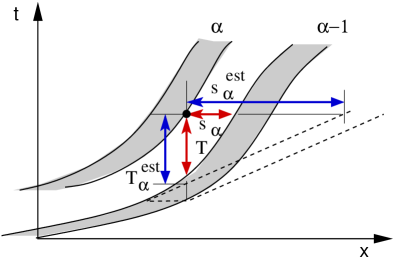
Figure 3: Left: Virtual detectors in the space-time-plot: Stationary detectors (loop detectors) correspond to lines parallel to the time axis while momentary detectors (aerial photographs) correspond to lines parallel to the space axis. Right: Illustration of the time gap $T^{\text{est,pt}}_{\alpha}$ according to Eq. (10) assuming constant velocities and the real time gap $T$ (please note that $T^{\text{est,pt}}_{\alpha}$ is an estimate from stationary measurement while $T^{\text{est,mom}}_{\alpha}$ as defined in Eq. (12) is an estimate from momentary measurement).

Assuming double loop detectors for the stationary measurement, the passage times $t_{\alpha}$ and $t_{\alpha-1}$ of vehicle $\alpha$ and $\alpha-1$ and their velocities at the time of passing the detector are available: $v_{\alpha}(t_{\alpha})$, $v_{\alpha-1}(t_{\alpha-1})$. Furthermore, we know the length of the leading vehicle $l_{\alpha-1}$ and, of course, the positions (front bumper) at the time of passing the detector: $x_{\alpha}(t_{\alpha})=x_{\alpha-1}(t_{\alpha-1})$.

From the momentary measurement at time $t_{\alpha}$ we obtain the positions of the two vehicles, $x_{\alpha}(t_{\alpha})$ and $x_{\alpha-1}(t_{\alpha})$, as well as the length of the leading vehicle $l_{\alpha-1}$. Assuming that we take two consecutive photographs, we can also determine the velocities $v_{\alpha}(t_{\alpha})$ and $v_{\alpha-1}(t_{\alpha})$. From this momentary measurement, the following spatial quantities can be calculated:

$$\text{Spatial gap }\quad s_{\alpha}(t_{\alpha}) =x_{\alpha-1}(t_{\alpha})-x_{\alpha}(t_{\alpha})-l_{\alpha-1},$$ (6)

$$\text{Approaching rate }\Delta v_{\alpha}(t_{\alpha}) =v_{\alpha}(t_{\alpha})-v_{\alpha-1}(t_{\alpha}).$$ (7)

Assuming constant velocities within the time interval $\Delta t_{\alpha}=t_{\alpha}-t_{\alpha-1}$, we can estimate the same quantities from data collected by a stationary detector:

$$s^{\text{est}}_{\alpha}(t_{\alpha}) =v_{\alpha-1}(t_{\alpha-1})\,\Delta t_{\alpha}-l_{\alpha-1},$$ (8)

$$\Delta v^{\text{est}}_{\alpha}(t_{\alpha}) =v_{\alpha}(t_{\alpha})-v_{\alpha-1}(t_{\alpha-1}).$$ (9)

Furthermore, the time gap $T$ defined by the gap related to the actual velocity, $s/v$, is a crucial quantity for the safety and capacity of traffic flow. From the time interval between two vehicles passing the stationary detector, $\Delta t_{\alpha}=t_{\alpha}-t_{\alpha-1}$, we can estimate the time gap while passing the detector:

$$T^{\text{est,pt}}_{\alpha}(t_{\alpha})=\Delta t_{\alpha}-\frac{l_{\alpha-1}}{v_{\alpha-1}(t_{\alpha-1})}.$$ (10)

This definition assumes constant velocity of the leading vehicle in the time interval $\Delta t_{\alpha}$. The “real” time gap, however, would be obtained by measuring the time where the rear bumper of the leading vehicle passed the detector:

$$T_{\alpha}(t_{\alpha})=t_{\alpha}-t^{\prime}\quad\text{with $t^{\prime}$ such that}\quad x_{\alpha-1}(t^{\prime})-l_{\alpha-1}=x_{\alpha}(t_{\alpha}).$$ (11)

Both quantities are illustrated in Fig. 3. Alternatively, we can estimate the time gap $T^{\text{est,mom}}$ from data collected by a momentary detector, again assuming constant velocities of the vehicles:

$$T^{\text{est,mom}}_{\alpha}(t_{\alpha})=\frac{s_{\alpha}(t_{\alpha})}{v_{\alpha-1}(t_{\alpha})}.$$ (12)

Data Preparation

In total, we have investigated 184,171 datapoints in the Prototype dataset and 722,904 in the two other datasets. Datapoints that were too close to the downstream boundary needed to be discarded since no spatial leader could be identified. Furthermore, we ignored datapoints that were closer than $3\,\mathrm{s}$ to a lane-changing event, leaving us with 146,213 datapoints from the Prototype dataset and 675,660 from the I-80 and US-101 datasets.

Due to tracking or vehicle dimension detection errors, some spatial and time gaps are negative or very small. A small spatial gap $s_{\alpha}$ leads to a very large inverse time-to-collision $\tau_{\alpha}$ (see below) which would dominate any higher-order moments of the $\tau_{\alpha}$ distribution. Thus, we filtered the data such that $s_{\alpha}\geq 1\,\mathrm{m}$ and $T_{\alpha}=\geq 0.1\,\mathrm{s}$ holds for every datapoint. This filter removed further 3,070 datapoints (2.1%) from our Prototype dataset extract and 11,755 (1.7%) from the extract of the two later datasets.

Microscopic Fundamental Diagram and Stopped Traffic

From the spatiotemporal measurements described above we can derive the inverse of the space headway, $(\Delta x_{\alpha})^{-1}=(x_{\alpha-1}-x_{\alpha})^{-1}$, and the inverse of the time headway, $(\Delta t_{\alpha})^{-1}$. These quantities are more intuitively described as “microscopic density” and “microscopic flow”, respectively, and will be referred to by these names throughout this section. For the Prototype dataset and the combined other two datasets, we plotted the distribution of velocity and microscopic density in Fig. 4 (top row). One clearly sees that the Prototype dataset mainly features free traffic and some bound traffic while the two later datasets feature only bound and jammed traffic. Plotting microscopic flow vs. microscopic density for all three data sets, we obtain the fundamental diagram (Fig. 4, bottom left). The free flow part of the diagram is completely provided by the Prototype dataset and the bound and jammed part is almost completely provided by the I-80 and US-101 datasets. Notice that, in contrast to the Prototype dataset, the later two sets exhibit stripes corresponding to the “preferred velocities” as seen in Fig. 1, which are much more prominent when applying the same procedure to the original, unsmoothed data.

From the rich amount of data in the jammed traffic regime it is also possible to determine the average headway of standing vehicles. We extracted all datapoints with velocities $v_{\alpha}<0.05\,\mathrm{m/s}$ and plotted the distribution of $\Delta x_{\alpha}$ in Fig. 4 (bottom right). The mode is at approximately $7\,\mathrm{m}$ for cars and $8\,\mathrm{m}$ for trucks (with a smaller second peak at $14\,\mathrm{m}$). However, the distribution is right-skewed, so that the mean values are a little higher: $8.3\,\mathrm{m}$ for cars and $9.7\,\mathrm{m}$ for trucks. Note that, for principal reasons, this distribution cannot be obtained from stationary detector data.

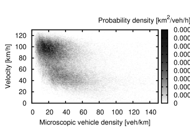
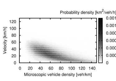
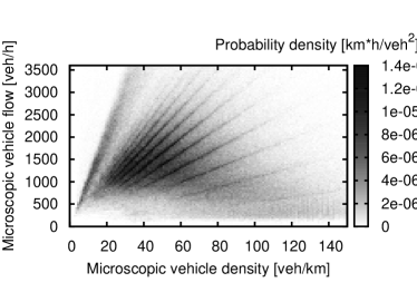
Figure 4: Probability density of the two-dimensional distribution (i.e., a “two-dimensional histogram”) of the microscopic density $(x_{\alpha-1}-x_{\alpha})^{-1}$ vs. velocity $v_{\alpha}$ in the Prototype dataset (upper left) and the two later I-80 and US-101 datasets (upper right). In the bottom left plot, the probability density of the microscopic density vs. microscopic flow $T_{\alpha}^{-1}$ is shown. The bottom right figure shows the probability density of the distribution of headways $x_{\alpha-1}-x_{\alpha}$ in stopped traffic ($v_{\alpha}<0.05\,\mathrm{m/s}$). The mean value is $8.3\,\mathrm{m}$ for cars and $9.9\,\mathrm{m}$ for trucks.

Time Gap Distribution

Let us now look at the time gaps as defined in the Eqs. (10) – (12). In Fig. 5 we have plotted the time gap distribution in three different traffic regimes: free traffic ($v>22.2\,\mathrm{m/s}$), jammed traffic ($v<15\,\mathrm{m/s}$), and bound traffic (intermediate velocities). Furthermore, in every plot, the real time gap $T_{\alpha}$ defined by Eq. (11) as obtained from the trajectories is compared to the estimated time gap from momentary measurement $T^{\text{est,mom}}_{\alpha}$ (cf. Eq. (12)). The first thing to note is the remarkable indifference of the distributions to the measurement method. For comparison we have also plotted the spatial gap distribution in jammed traffic (Fig. 5, top right), which the stationary measurements shifts to larger values. In the other two traffic regimes the spatial gap distributions agree very well.

Furthermore, it can be seen that the mode of the time gap distribution shifts from approximately $1.5\,\mathrm{s}$ in jammed traffic to $1\,\mathrm{s}$ in free traffic. This effect is also visualized in the middle right plot of Fig. 5. The mean time gap is $2.6\,\mathrm{s}$ in jammed traffic, $1.9\,\mathrm{s}$ in bound traffic, and $2.0\,\mathrm{s}$ in free traffic. In the bottom right plot we visualized another dependency of the time gap: Although data becomes sparse towards larger values, there is a significant tendency towards larger time gaps if the velocity difference to the leading vehicle is large (regardless of whether approaching the vehicle or falling behind).

Besides comparing time gaps measured by stationary detectors with time gaps measured momentary detectors, there are also different ways to determine the time gap with a stationary detector. The real time gap is the time between the leader’s rear bumper and the own front bumper passing the detector (Eq. (11)). However, if detectors only produce passage times and vehicle lengths and velocities, one needs to estimate the timegap from the passage by assuming constant velocity of the leader vehicle while passing the detector (Eq. (10)). This error is very small in most cases: only 10% of our sample datapoints had an error in the estimate from passage times $T^{\text{est,pt}}_{\alpha}$ that exceeded 10% of the real time gap $T_{\alpha}$.

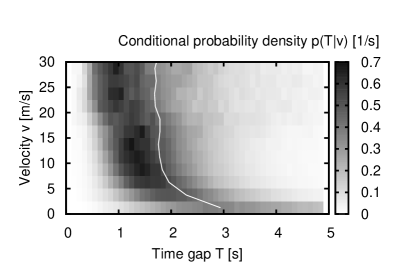
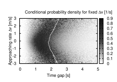
Figure 5: The left column shows the distribution of time gap $T_{\alpha}$ in the different traffic regimes. In the right column, we plotted the distribution of the spatial gap $s_{\alpha}$ in jammed traffic (top), the distribution of the time gap for different given velocities $v_{\alpha}$ (middle), and the distribution of the time gap for different given approaching rates $\Delta v_{\alpha}$ (bottom). The white lines show the mean value for each row of the plot, i.e. the mean of the time gap for different values of $v$ or $\Delta v$.

Time-to-Collision

Another relevant quantity is the time-to-collision (TTC) which serves as safety measure for traffic situations as it states the time left until the vehicle will crash into its leader unless at least one of the drivers changes speed [16, 17]. The TTC as a spatial quantity is defined by Eqs. (6) and (7) as

$$\tau_{\alpha}(t_{\alpha})=\frac{s_{\alpha}(t_{\alpha})}{\Delta v_{\alpha}(t_{\alpha})}.$$ (13)

The TTC can also be estimated from stationary (temporal) measurements (8) and (9):

$$\tau_{\alpha}^{\text{est}}(t_{\alpha})=\frac{s_{\alpha}^{\text{est}}(t_{\alpha})}{v_{\alpha}(t_{\alpha})-v_{\alpha-1}(t_{\alpha-1})}.$$ (14)

We will now investigate the impact of the constant-velocity assumption used to derive the TTC $\tau_{\alpha}^{\text{est}}$ from stationary measurements. Since the TTC diverges for $\Delta v_{\alpha}=0$, it is more convenient to discuss the TTC in terms of its inverse $\tau_{\alpha}^{-1}=\Delta v_{\alpha}/s_{\alpha}$.

In Fig. 6 we plotted the distribution of the inverse TTC in the Prototype dataset (left) and in the two later datasets (right). In contrast to the spatial and time gap distributions, the inverse TTC distribution differs significantly between the two measurement methods. The inverse TTC is sensitive to errors in the spatial gap, especially when the gap is small. Therefore, we ignored inverse TTC values with absolute value larger than $1$ when computing statistical properties of the distributions. In this way, we ignored 0.59% of all datapoints.

The mean of the absolute error $\Delta\tau_{\alpha}^{-1}:={(\tau_{\alpha}^{\text{est}})}^{-1}-\tau_{\alpha}^{-1}$ is $0.00098$ in the Prototype dataset and $-0.0134$ in the two later datasets. The same can be observed when splitting the data from all datasets into traffic regimes as described above. The mean error is $0.000045$ in jammed traffic, $-0.0067$ in bound traffic, and $-0.0122$ in free traffic. The variance of the errors is strongest in jammed traffic ($0.0236$), while it is $0.00388$ in bound traffic, and $0.00225$ in free traffic. Statistical properties of the inverse TTC distributions have been collected into Table 1. One should especially note that the skewness is consistently shifted towards higher values by the stationary measurement. This is visible in the plots as well.

In view of the application of the TTC as safety measure, it is particularly critical that stationary measurements consistently decrease the probability of measuring a large positive inverse-time-to-collision value which corresponds to a small positive $\tau_{\alpha}$ indicating a dangerous traffic situation. For example in free traffic (cf. Fig. 7), the fraction of positive TTC values below $5\,\mathrm{s}$ (0.8% of the datapoints) which is considered as critical [16, 17] is underestimated by the stationary measurement by about a factor of $2$. Thus, stationary measurements tend to euphemize the danger of collision.

Figure 6: Distribution of the inverse time-to-collision $\tau_{\alpha}^{-1}$ in the Prototype dataset (left) and the two later datasets (right) compared to the estimated time-to-collision ${(\tau_{\alpha}^{\text{est}})}^{-1}$ obtained from stationary measurements. The upper figures show both distributions while the lower figures show the distributions of the measurement errors $\Delta\tau_{\alpha}^{-1}={(\tau_{\alpha}^{\text{est}})}^{-1}-\tau_{\alpha}^{-1}$.

Figure 7: The figure shows distributions of the inverse time-to-collision $\tau_{\alpha}^{-1}$ of all data sets in different traffic phases compared to the estimated time-to-collision ${(\tau_{\alpha}^{\text{est}})}^{-1}$ obtained from stationary measurements.

Dataset	Mean	Variance	Skewness	Sign change
Prototype	0.00874006 -0.00462994	0.00706569 0.00422629	-0.264358 0.16407	19.2402% 7.63705%
I-80/US-101	-0.00640645 -0.00542511	0.0122408 0.0120666	0.0109132 1.58624	23.0413% 21.3802%
jammed traffic	-0.00637853 -0.00633317	0.0124101 0.0121906	-0.000798933 1.54999	23.6459% 21.1149%
bound traffic	0.00624585 -0.000502914	0.00699072 0.00348709	-0.204996 0.798759	15.0853% 10.7964%
free traffic	0.0126101 0.000389615	0.00483055 0.00260696	0.179115 0.459587	16.6644% 5.58995%

Table 1: Statistical properties of the inverse TTC distributions in the different datasets. In the mean, variance, and skewness column, the top value is obtained from momentary measurements (the real value), while the bottom value is obtained from stationary measurements (the estimated value). In the sign change column, the top value states the amount of datapoints for which the stationary measurement determines a positive time-to-collision while the momentary measurement determines a negative value. The bottom value gives the amount of datapoints for which the sign change is the other way round. The jammed, bound, and free traffic dataset are combined from the Prototype and the two later NGSIM datasets. A datapoint was assigned to jammed traffic if the vehicle’s velocity was below $15\,\mathrm{m/s}$, to free traffic if $v_{\alpha}>22.2\,\mathrm{m/s}$, and to bound traffic, otherwise.

Lane Changes

Besides the ability to compare stationary and momentary measurements, the NGSIM trajectory data sets also provide a good basis to investigate lane changes. In order to determine the lane change duration, we collected all lane changes in the NGSIM data. However, from the processed video data supplied with the NGSIM datasets it can be seen that sometimes the tracking algorithm accidentally misplaced a vehicle across the lane boundary and back after a few timesteps. Also, sometimes drivers might have abort an already begun lane change or quickly crossed two lanes. Since we just want to look at real and normal single-lane lane changes, we therefore filtered out all lane changes that were closer than a certain threshold $\tau_{\text{th}}$ to another lane change, which we chose to be $\tau_{\text{th}}=5\,\mathrm{s}$. We also sorted out lane changes that did not involve one of the four left-most lanes in order to reduce the effect of the on-/off-ramp on our lane change analysis.

The former criterion was chosen to sort out cases where drivers aborted an already begun lane change or where the tracking algorithm accidently misplaced a vehicle across the lane boundary. The latter criterion ensures that we look at discretionary lane changes only.

With $\lambda_{\alpha}(t)$ denoting the lane used by vehicle $\alpha$ at time $t$, a lane-changing event occurs at time $t_{\text{lc}}$ if $\lambda_{\alpha}(t_{\text{lc}})\neq\lambda_{\alpha}(t_{\text{lc}}+\Delta t)$ (where $\Delta t$ is the time interval between two consecutive datapoints of a trajectory). For each lane-changing event, we extracted a 20-second-environment of the trajectory with time, longitudinal and lateral position relative to the lane-changing event:

Relative time $$\tau:=t-t_{\text{lc}},$$ (15)

Relative longitudinal position $$\xi_{\alpha}(\tau):=x_{\alpha}(\tau+t_{\text{lc}})-x_{\alpha}(t_{\text{lc}}).$$ (16)

Relative lateral position $$\eta_{\alpha}(\tau):=y_{\alpha}(\tau+t_{\text{lc}})-y_{\alpha}(t_{\text{lc}}).$$ (17)

Then, we are able to produce a plot of the conditional probability density $p(\eta|\tau)$ that a vehicle is at a relative lateral position $\eta$ at a certain time $\tau$ relative to the lane-changing event time (Fig. 8, top). From this, we can roughly estimate the lane change duration to approximately $5-6\,\mathrm{s}$ by looking at the curvature of the two mode values $\hat{\eta}_{+}(\tau):=\mathop{\text{arg}\,\text{max}}_{\eta>0}\{p(\eta|\tau)\}$ and $\hat{\eta}_{-}(\tau):=\mathop{\text{arg}\,\text{max}}_{\eta<0}\{p(\eta|\tau)\}$. This procedure is similar to the approach done in Ref. [7], where the lane change start and end time of each trajectory were determined by looking at the curvature of the lateral position $y_{\alpha}(t)$. However, finding the correct point in the curvature might be somewhat arbitrary, thus we will in the following look at a more well-defined way to measure a lower bound of the lane change duration.

The NGSIM vehicle detection algorithm does not only detect the vehicle position but also its length $l_{\alpha}$ and width $w_{\alpha}$. Since the lane assignment algorithm works such that each datapoint is placed into the lane where its mid-point front-bumper position $(x_{\alpha},y_{\alpha})$ lies in, it is possible to determine the time where a lane-changing vehicle first intruded the destination lane and the time where it just completely left the source lane. Given the lane-changing event time $t_{\text{lc}}$ and the relative time and position as defined in Eqs. (15)–(17), the relative start time $\tau_{\text{s}}$ and end time $\tau_{\text{e}}$ of the lane change may be defined as follows (a higher lane index $\lambda_{\alpha}$ corresponds to a larger lateral position $\eta_{\alpha}$):

$$\tau_{\text{s}} =\begin{cases}\max\{\tau\mid\tau<0\,\text{and}\,\eta_{\alpha}(\tau)+w_{\alpha}/2<0\}&\text{if }\lambda_{\alpha}(t_{\text{lc}})<\lambda_{\alpha}(t_{\text{lc}}+\Delta t),\\ \max\{\tau\mid\tau<0\,\text{and}\,\eta_{\alpha}(\tau)-w_{\alpha}/2>0\}&\text{otherwise}.\end{cases}$$ (18)

$$\tau_{\text{e}} =\begin{cases}\min\{\tau\mid\tau<0\,\text{and}\,\eta_{\alpha}(\tau)-w_{\alpha}/2>0\}&\text{if }\lambda_{\alpha}(t_{\text{lc}})<\lambda_{\alpha}(t_{\text{lc}}+\Delta t),\\ \min\{\tau\mid\tau<0\,\text{and}\,\eta_{\alpha}(\tau)+w_{\alpha}/2<0\}&\text{otherwise}.\end{cases}$$ (19)

Then, of course, the lane change duration is obtained trivially from

$$T_{\text{lc}}=\tau_{\text{e}}-\tau_{\text{s}}.$$ (20)

In total, we have investigated 1231 lane changes, 1105 of which were suitable to calculate $T_{\text{lc}}$ according to Eq. (20). In the remaining 126 cases, either $\tau_{\text{s}}$ or $\tau_{\text{e}}$ were undefined because the corresponding condition was not fulfilled for any $\tau\in[-10,10]$ within the 20-second-environment around the lane change. This can be attributed to vehicle dimension detection errors or vehicle tracking errors, both leading to a trajectory where the vehicle drives on the lane boundary for some time. Figure 8 (bottom left) shows the distribution of the lane change duration of the examined lane changes. One immediately notices that most lane changes take somewhat about $3\,\mathrm{s}$ (mode value of the distribution), a value already found valid for German highways back in 1978 [18], which is, however, substantially different from the one obtained by rule of thumb from the conditional probability density $p(\eta|\tau)$. The mean and standard variation of the distribution are

$$\bar{T}_{\text{lc}}=4.01\pm 2.31\,\mathrm{s}.$$ (21)

However, one should be aware that definition (20) measures the time span where the vehicle occupies two lanes, which can only be taken as a lower bound of the real lane change duration. Including the preparation and possible post-processing of a lane change, a value of $5-6\,\mathrm{s}$ might seem realistic. Since the “real” beginning of a lane change, the decision for making the lane change, is impossible to measure, and the “physical’ beginning, the moment where the driver starts to turn the wheel, is very difficult if not impossible to measure, we think that our proposed definition is a good estimator for the lane change duration, because it uses well-defined and easily measurable quantities.

In the lower right, Fig. 8 shows the conditional probability density of the velocity difference between the leader on the destination lane and the leader on the source lane for different fixed times relative to the lane-changing event. As indicated by the white line, the mean value rises before the lane change by approximately $1\,\mathrm{m/s}$. This indicates that drivers perceive a velocity advantage on the destination lane before performing the lane-changing maneuver and take anticipationary actions.

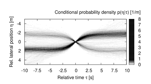
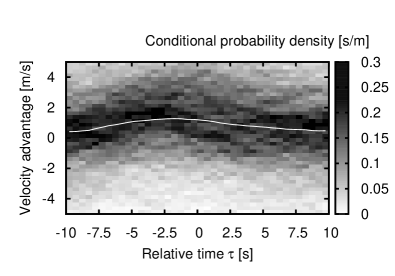
Figure 8: Lane changes: The upper plot shows the conditional probability $p(\eta|\tau)$ of finding a vehicle on lateral position $\eta$ relative to the lane boundary at a given time $\tau$ relative to the lane-changing event time. The lower left plot shows the distribution of lane change durations $T_{\text{lc},\alpha}$ according to the definition (20) given in the text. The mean lane change duration is $\bar{T}_{\text{lc}}=(4.01\pm 2.31)\,\mathrm{s}$. The lower right plot shows the conditional probability density of the velocity difference between the leader on the destination lane and the leader on the source lane for fixed times relative to the lane-changing event (the white line shows the mean value).

Discussion and Future Research

The availability of the NGSIM data sets spurred a considerable research activity, particularly with respect to lane changing, where larger-scale empirical investigations are now possible for the first time. To date, most researchers only used the positional information which allows, for example, to investigate the lane-changing rate, the duration of lane changes, the gap-acceptance behavior, or the propagation velocity of longitudinal density waves.

The full potential of the data, i.e., using the positional information together with that for velocity and acceleration, has hardly been tapped. A possible reason is that the velocity and acceleration information cannot be used directly since the noise of the positional information is greatly increased by the necessary numerical differentiations. In this paper, we have developed a filter to extract more realistic velocity and acceleration information from the positional data. Since the trajectories are comparatively short, we included the boundary regions in the filtered output by reducing the width of the necessary smoothing operations near the boundary. This implies determining the most efficient order of the smoothing and differentiation operations of the filter since they do no longer commute, and a wrong order may even lead to a systematic bias.

It must be noticed that it is inherently difficult to determine the optimal filter parameters that eliminate most of the noise while retaining the real information. This is particularly crucial for mean-reverting quantities such as the accelerations, where large smoothing time intervals will eventually suppress the whole information. Clearly, further research is necessary to develop more sophisticated, possibly nonlinear, filters.

The velocity and acceleration information of the trajectories can be used in many ways. In this work, we investigate the systematic errors in determining spatial quantities from temporal information, and vice versa. The background is that spatial quantities such as the gap to the leading vehicle, the density, or the times-to collision, are usually estimated by single-vehicle data from stationary detectors, i.e., by using temporal information. Using “virtual stationary detectors” that are fed with the trajectory data and simulating the estimation procedure, we could quantitatively determine the resulting estimation errors. Besides the well-known underestimation of the real density of congested traffic, we found that the percentage of critical values of times-to-collision is underestimated by a factor of 2 and more when estimated from single-vehicle data. This clearly is relevant for safety-related applications.

Another application field are empirical tests and parameter calibrations for car-following and lane-changing models. In this work, we showed that, prior to a discretionary lane change, there is a noisy and small, but significant, velocity difference in favor of the target lane. From this, we conclude that lane-changing decisions are not only based on gaps and velocities, but also on velocity differences, and possibly, on accelerations as considered in Ref. [19].

More generally, the trajectory data allow, for the first time, to empirically investigate the strategical and tactical actions for preparing or facilitating a lane change [19]. Apart from the actions of the lane-changing driver, this also includes the actions of the other drivers involved, such as cooperative actions of the follower on the target lane to allow zip-like merging. This is relevant for microscopic simulation software since it turned out to be notoriously difficult to model realistic lane changes, particularly in the case of mandatory changes in congested traffic.

The acceleration information of the data can also be used to investigate to which extent the local traffic environment (consisting, e.g., of the next-nearest and further leading vehicles) influences the longitudinal driving behavior [20]. For example, it has been proposed that the driving style is influenced by the local velocity variance as determined from few leading vehicles [21].

Finally, the velocity and acceleration information can be used to determine the influence of traffic congestion on the fuel consumption and emissions [15]. Since reliable characteristic maps are available for the instantaneous fuel consumption and emission rates of various pollutants as a function of velocity and acceleration, these quantities can now be estimated, for real situations, with unprecedented accuracy.

References

- [1] US Department of Transportation, “NGSIM – Next Generation Simulation,”, 2007, http://www.ngsim.fhwa.dot.gov – Access date: May 5, 2007.
- [2] A. Skabardonis, “Estimating and Validating Models of Microscopic Driver Behavior with Video Data,” Technical report, California Partners for Advanced Transit and Highways (PATH) (2005) .
- [3] X.-Y. Lu and A. Skabardonis, “Freeway Traffic Shockwave Analysis: Exploring the NGSIM Trajectory Data,” In TRB 2007 Annual Meeting CD-ROM, (2007).
- [4] R. P. Roess and J. M. Ulerio, “Analysis of Four Weaving Sections: Implications for Modeling,” In TRB 2007 Annual Meeting CD-ROM, (2007).
- [5] L. Zhang and V. Kovvali, “Freeway Gap Acceptance Behaviors Based on Vehicle Trajectory Analysis,” In TRB 2007 Annual Meeting CD-ROM, (2007).
- [6] V. Goswami and G. H. Bham, “Gap Acceptance Behavior in Mandatory Lane Changes under Congested and Uncongested Traffic on a Multi-lane Freeway,” In TRB 2007 Annual Meeting CD-ROM, (2007).
- [7] T. Toledo and D. Zohar, “Modeling duration of lane changes,” Transportation Research Record 1999, 71–78 (2007).
- [8] C. F. Choudhury, M. E. Ben-Akiva, T. Toledo, G. Lee, and A. Rao, “Modeling Cooperative Lane Changing and Forced Merging Behavior,” In TRB 2007 Annual Meeting CD-ROM, (2007).
- [9] L. Leclercq, N. Chiabaut, J. Laval, and C. Buisson, “Relaxation phenomenon after lane changing: Experimental validation with NGSIM dataset,” Transportation Research Record 1999, 79–85 (2007).
- [10] T. Vu, R. Roess, J. Ulerio, and E. Prassas, “Simulation of a weaving section,” In TRB 2007 Annual Meeting CD-ROM, (2007).
- [11] W.-L. Jin and L. Li, “A study of first-in-first-out violation in freeway traffic,” In TRB 2007 Annual Meeting CD-ROM, (2007).
- [12] N. A. Webster, T. Suzuki, E. Chung, and M. Kuwahara, “Tactical Driver Lane Change Model Using Forward Search,” In TRB 2007 Annual Meeting CD-ROM, (2007).
- [13] C. Alecsandru and S. Ishak, “Accounting for random driving behavior and nonlinearity of backward wave speeds in the cell transmission model,” In TRB 2007 Annual Meeting CD-ROM, (2007).
- [14] A. Kesting and M. Treiber, “Calibrating Car-Following Models using Trajectory Data: Methodological Study,” Transportation Research Record (2008), in print.
- [15] M. Treiber, A. Kesting, and C. Thiemann, “How Much do Traffic Congestion Increase Fuel Consumption and Emissions? Applying a Fuel Consumption Model to the NGSIM Trajectory Data,” In TRB Annual Meeting 2008 CD-ROM, (Transportation Research Board of the National Academies, Washington, D.C., 2008).
- [16] S. Hirst and R. Graham, “The Format and Presentation of Collision Warnings,” in Ergonomics and Safety of Intelligent Driver Interfaces, Y. Noy, ed., (Lawrence Erblaum Associates, New Jersey, 1997).
- [17] M. M. Minderhoud and P. H. L. Bovy, “Extended time-to-collision measures for road traffic safety assessment,” Accident Analysis & Prevention 33, 89–97 (2001).
- [18] U. Sparmann, “Spurwechselvorgänge auf zweispurigen BAB-Richtungsfahrbahnen,” Forschung Straßenbau und Straßenverkehrstechnik 263 (1978).
- [19] A. Kesting, M. Treiber, and D. Helbing, “General Lane-Changing Model MOBIL for Car-Following Models,” Transportation Research Record 1999, 86–94 (2007).
- [20] M. Treiber, A. Kesting, and D. Helbing, “Delays, inaccuracies and anticipation in microscopic traffic models,” Physica A 360, 71–88 (2006).
- [21] M. Treiber, A. Kesting, and D. Helbing, “Understanding widely scattered traffic flows, the capacity drop, and platoons as effects of variance-driven time gaps,” Physical Review E 74, 016123 (2006).