Analytic approach to bifurcation cascades
in a class of generalized Hénon-Heiles potentials

Abstract

We investigate the bifurcation cascades of a linear librational orbit in a generalized class of Hénon-Heiles potentials. The stability traces of the new orbits born at its bifurcations are found numerically to intersect linearly at the saddle energy ($e=1$), forming what we term the ‘‘Hénon-Heiles fans’’. In the limit close to the saddle energy ($e\to 1$), where the dynamics is nearly chaotic, we derive analytical asymptotic expressions for the stability traces of both types of orbits and confirm the numerically determined properties of the generalized ‘‘Hénon-Heiles fans’’. As a bonus of our results, we obtain analytical approximations for the bifurcation energies $e_{n}$ which become asymptotically exact for $e_{n}\to 1$.

I Introduction

The approximation of the exact density of states of a quantum system in terms of classical periodic orbits via semiclassical trace formulae is a fascinating subject which has triggered a lot of research (see gubu ; book and the literature quoted therein). It presents a nice illustration of the correspondence between classical and quantum mechanics, besides allowing one to approximately determine quantum shell structures in terms of classical mechanics (see book for applications in various fields of physics). In Hamiltonian systems which are classically neither regular nor purely chaotic, this semiclassical theory is enriched – but also complicated – by the many facets of non-linear dynamics. One of them is the bifurcation of periodic orbits when they undergo changes of stability ozob .

An essential ingredient to determine the stability of a periodic orbit is its so-called stability matrix ${\rm M}_{\perp}$, appearing in the amplitudes of Gutzwiller’s trace formula gutz , which is determined from the linearized equations of motion around the periodic orbit. The analytical calculation of ${\rm M}_{\perp}$ for non-integrable systems with mixed dynamics is in general not possible; the only non-trivial example is, to our knowledge, that of a two-dimensional quartic oscillator yosh .

In this paper we investigate the stability matrix ${\rm M}_{\perp}$ of the simplest orbit in a class of two-dimensional potentials which are a generalization of the famous Hénon-Heiles (HH) potential hhpa that has become a text-book example of a system with mixed classical dynamics. For small energies the motion is dominated by a harmonic-oscillator part and is quasi-regular; at energies close to and above the saddles ($e=1$), over which a particle can escape, the motion is quasi-chaotic (see, e.g., gubu ; book ; hhpa ; ford and the literature quoted therein). At all energies below the saddle, there exists a straight-line librating orbit A oscillating towards one of the saddles. This orbit undergoes an infinite sequence of stability oscillations and hence a cascade of bifurcations, which can be understood as the main mechanism of the transition from regular motion to chaos davb ; mbgu ; lamp . The stability traces of the new orbits R and L generated at the bifurcations are found numerically mbgu to intersect linearly at the saddle energy ($e=1$), forming what was termed the ‘‘Hénon-Heiles fans’’ bkwf .

In the present paper we present analytical calculations of the stability traces of both the A orbit and the new orbits R and L bifurcating from it. The results are obtained in the limit close to the saddle ($e\to 1$) and hence asymptotically valid as the bifurcation energies $e_{n}$ approach the saddle energy $e=1$. They confirm analytically the numerical properties of the ‘‘Hénon-Heiles fans’’ also in the generalized HH potential. As a bonus, we obtain analytical expressions for the bifurcation energies $e_{n}$, which are mathematically valid asymptotically for $e_{n}\to 1$, i.e., for $n\to\infty$, and practically for $n\geq 7$ within 5 digits.

In Sec. II we present the generalized Hénon-Heiles system and discuss its shortest orbits, the bifurcation cascade of the linear A orbit and, in particular, the properties of the ‘‘Hénon-Heiles fans’’. In Sec. III we present the basic ideas of our analytical approach and the essential results, while the technical details of our calculations are given in the Appendices A and B. In Sec. IV we present an alternative perturbative approach for evaluating the stability traces, with the details given in Appendix C, and compare its results with those of the non-perturbative calculations.

II Bifurcation cascades in the Hénon-Heiles system

II.1 The generalized Hénon-Heiles Hamiltonian

In this paper we investigate the following family of Hamiltonians:

$$H_{GHH}=\frac{1}{2}\,(p_{x}^{2}+p_{y}^{2})+\frac{1}{2}\,(x^{2}+y^{2})+\alpha\left[-\frac{1}{3}\,y^{3}+\gamma\,x^{2}\,y\right]\!,$$ (1)

where $\gamma\geq 0$ is a parameter specifying specific members of the family, and $\alpha>0$ is a chaoticity parameter that can be scaled away with the energy as shown below. For $\gamma=1$, the Hamiltonian (1) reduces to the standard Hénon-Heiles (HH) Hamiltonian hhpa ; we therefore call (1) here the ‘‘generalized Hénon-Heiles’’ (GHH) Hamiltonian. The HH system with $\gamma=1$ has C_3v symmetry: it is invariant under rotations around the origin by $2\pi/3$ and $4\pi/3$, and under reflections at three symmetry lines with the angles $\pm\pi/6$ and $\pi/2$ with respect to the $x$ axis. It exhibits three saddles at energy $E_{sad}=1/6\alpha^{2}$, the equipotential lines at $E=E_{sad}$ forming an equilateral triangle. For $\gamma\neq 1$, the C_3v symmetry is lost and only the reflection symmetry at the $y$ axis remains; there are, however, still three saddles over which the particle can escape. For $\gamma=0$ the system becomes separable and has only one saddle on the $y$ axis (cf. jkmb ; maf ).

After multiplying the Hamiltonian (1) by a factor $6\alpha^{2}$ and introducing the scaled variables $x^{\prime},y^{\prime},e$ by

$$x^{\prime}=\alpha x\,,\qquad y^{\prime}=\alpha y\,,\qquad e=6\alpha^{2}E=E/E_{sad}\,,$$ (2)

the scaled Hamiltonian becomes independent of $\alpha$, and for a given $\gamma$ there is only one parameter $e$ that regulates the classical dynamics. For simplicity of notation, we omit in the following the primes of the scaled coordinates $x,y$ but keep using the scaled energy $e$.

For $\gamma=1$, the three saddles are at the scaled energy $e=1$; one of them is positioned at $x=0$, $y=1$. For $\gamma\neq 1$, the saddle with energy $e=1$ persists at the same position, while the two other saddles lie at different energies and are positioned symmetrically to the $y$ axis. For a more detailed description of the topology of the potential (1) (and an even larger class of generalized HH potentials) and its shortest periodic orbits, we refer to a forthcoming publication bttb .

The shortest periodic orbits of the standard HH system ($\gamma=1$) have been extensively discussed in the literature chur ; davb ; mbgu ; lamp , and their use in semiclassical trace formulae for the quantum density of state of the HH system was investigated in bblm ; hhun ; jkmb ; jkwb .

II.2 The motion along the A orbit

As mentioned above, we use henceforth the symbols $x,y$ for the scaled coordinates (corresponding to $\alpha=1$), along with the scaled energy $e$ given in (2). The equations of motion for the Hamiltonian (1) are then

$$\ddot{x}(t)+[1+2\gamma\,y(t)]\,x(t) = 0\,,$$ (3)

$$\ddot{y}(t)+y(t)-y^{2}(t)+\gamma\,x^{2}(t) = 0\,.$$ (4)

In the present work we focus on the linear orbit that librates along the $y$ axis, here called the A orbit. It goes through the origin $(x,y)=(0,0)$ and towards the saddle at $(x,y)=(0,1)$ which it, however, only reaches asymptotically for $e\to 1$ with a period $T_{A}\to\infty$. Since this orbit has $x_{A}(t)={\dot{x}}_{A}(t)=0$ at all times $t$, its equation of motion is

$$\ddot{y}_{A}(t)+y_{A}(t)-y_{A}^{2}(t)=0\,,$$ (5)

which can be solved analytically jkmb . We give here the result in the most general form, relevant for our following development, where the initial point along the $y$ axis is given as $y_{0}=y_{A}(t=0)$. The solution is then:

$$y_{A}(t)=y_{1}+(y_{2}-y_{1})\,{\rm sn}^{2}(z,\kappa)\,,$$ (6)

$$z=a_{\kappa}t+F(\varphi,\kappa)\,.$$ (7)

Here ${\rm sn}(z,\kappa)$ is a Jacobi elliptic function grry with argument $z$; its modulus $\kappa$ and the constant $a_{\kappa}$ are given by

$$\kappa=\sqrt{\frac{y_{2}-y_{1}}{y_{3}-y_{1}}}\,,\qquad a_{\kappa}=\sqrt{\left(y_{3}-y_{1}\right)\!/6}\,,$$ (8)

in terms of the three real solutions of the equation $e=3\,y^{2}-2\,y^{3}\leq 1$ given by

$$y_{1}=1/2-\cos(\pi/3-\phi/3)\,,\quad y_{2}=1/2-\cos(\pi/3+\phi/3)\,,\quad y_{3}=1/2+\cos(\phi/3)\,,$$ (9)

with $\cos\phi=1-2\,e$. The function $F(\varphi,\kappa)$ in (6) is the incomplete elliptic integral of first kind with modulus $\kappa$, the argument $\varphi$ being determined by the initial condition:

$$\varphi=\arcsin\sqrt{\frac{y_{0}-y_{1}}{y_{2}-y_{1}}}\,.$$ (10)

$y_{1}$ and $y_{2}$ are the lower and upper turning points, respectively, of the A orbit along the $y$ axis. The period and the action of the (primitive) A orbit are given by

$$T_{A}(e)=\frac{2}{a_{\kappa}}\,\hbox{\bf K}(\kappa)\,,\qquad S_{A}(e)=\frac{12\,a_{\kappa}}{5\,\alpha^{2}}\,[\hbox{\bf E}(\kappa)+c_{\kappa}\hbox{\bf K}(\kappa)]\,,$$ (11)

with $c_{\kappa}=-2(y_{3}-y_{2})(2\,y_{3}-y_{2}-y_{1})/9$, in terms of the complete elliptic integrals of first and second kind, $\hbox{\bf K}(\kappa)$ and $\hbox{\bf E}(\kappa)$ (we use the notation of grry ).

Note that in the limit $e\to 1$, we have $y_{2}\to 1$, $y_{3}\to 1$ and $\kappa\to 1$, so that $\hbox{\bf K}(\kappa)$ and $T_{A}$ diverge (while $S_{A}$ remains finite). The A orbit then is no longer periodic (and may be called a ‘‘homoclinic orbit’’ ozob ). Expanding $T_{A}$ around $e=1$, one finds the asymptotic form mbgu

$$T_{A}(e)\;\approx\;\widetilde{T}_{A}(e)={\rm ln}\left(\frac{432}{1-e}\right).\qquad(e\to 1)$$ (12)

II.3 The bifurcation cascade of the A orbit in the standard HH potential

While approaching the saddle as $e\to 1$, the A orbit undergoes an infinite cascade of pitchfork bifurcations, giving birth to a sequence of new orbits R₅, L₆, R₇, L₈, …. This scenario, which has some similarities to the Feigenbaum scenario feig , was discussed extensively in mbgu , and the analytical forms of the newborn R and L orbits in terms of periodic Lamé functions were discussed in lamp .

In Fig. 1 we show the traces of the stability matrix ${\rm M}_{\perp}$, defined in (14) below, of the A orbit and the orbits bifurcated from it, plotted versus energy $e$. Whenever ${\rm tr}\,{\rm M}_{\perp}=2$, a bifurcation occurs. We see the successive bifurcations at increasing energies $e_{n}$; upon repeated zooming the upper end of the energy scale near $e=1$ (from bottom to top), the pattern repeats itself in a self-similar manner. The bifurcation energies $e_{n}$ form a geometrically progressing series (see mbgu ; lamp for details). cumulating at the saddle energy ($e=1$) such that $e_{5}({\rm R}_{5})<e_{6}({\rm L}_{6})<e_{7}({\rm R}_{7})<\dots<1$, where the parentheses contain the names of the new orbits born at the pitchfork bifurcations. These are alternatively of R type (rotations) and of L type (librations). (The subscripts in the orbit names indicate the Maslov indices appearing in the semiclassical trace formulae; the index of the A orbit increases by one unit at each bifurcation.) Due to the discrete symmetries of the system, all these pitchfork bifurcations are isochronous and hence not generic (cf. bttb ).

In Fig. 2, we show again ${\rm tr}\,{\rm M}_{\perp}$ – in the following briefly termed the ‘‘stability traces’’ – of the same orbits, but this time plotted versus their respective periods $T$. On this scale, ${\rm tr}\,{\rm M}_{\perp A}(T_{\rm A})$ (shown by the heavy line) is numerically found davb for large $T_{\rm A}$ to go like a sine function; its period $\Delta T=3.6276$ was shown in mbgu to be given analytically by $\Delta T=2\pi/\!\sqrt{3}$. The exact calculation of the function ${\rm tr}\,{\rm M}_{\perp A}(T_{\rm A})$ is, however, not trivial at all. It is one of the objects of our present investigations (see Sec. III.2).

II.4 The ‘‘Hénon-Heiles fans’’

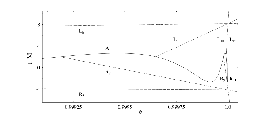
Figure 3: The ‘‘Hénon-Heiles fans’’. Trace of stability matrix of primitive A orbit (solid line) and the first four pairs of R orbits (dashed) and L orbits (dash-dotted) in the standard HH system, plotted versus scaled energy $e$; the latter forming two fans for the R and L orbits.

An interesting property of the stability traces of the R and L orbits born at the bifurcations, which has been observed numerically mbgu and termed the ‘‘Hénon-Heiles fan’’ structure bkwf , is emphasized in Fig. 3. Here we plot the stability traces of the primitive A orbit and the first three primitive pairs of R and L orbits versus the scaled energy $e$. We note two prominent features (which can also be recognized in Fig. 1):
($i$) The functions ${\rm tr}\,{\rm M}_{\perp R,L}(e)$ are approximately linear up to (and even beyond) the barrier energy $e=1$.
($ii$) The curves ${\rm tr}\,{\rm M}_{\perp R,L}(e)$ intersect at $e=1$ in one point each for all R and L type orbits with Maslov indices $>8$, positioned at the values $2\pm d$ with $d=6.183\pm 0.001$, thus forming two fans emanating from these points. The uncertainty in the parameter $d$ comes from the numerical difficulty of finding periodic orbits (which was done using a Newton-Raphson iteration procedure) close to bifurcations; our result for $d$ was obtained for R_n and L${}_{n^{\prime}}$ orbits with $9\leq n,n^{\prime}\leq 13$, evaluated at $e=1$. The upper limit $n=13$ is due to the numerical problems only; we expect that the same value $d=6.183\pm 0.001$ holds also for all higher $n$.

We found exactly the same types of ‘‘HH fans’’ for the generalized HH systems given by the Hamiltonian (1) for the bifurcation cascade of the A orbit along the $y$ axis, whereby the slopes of the fans and hence the value of $d$ depend on the parameter $\gamma$. The ‘‘GHH fans’’ can be described, for large enough $n$, by the empirical formula

$${\rm tr}\,{\rm M}_{\perp R,L}^{(emp)}(e)\;=\;2\mp c_{RL}(\gamma)\,\frac{(e-e_{n})}{(1-e_{n})}\,,\qquad(e\geq e_{n})$$ (13)

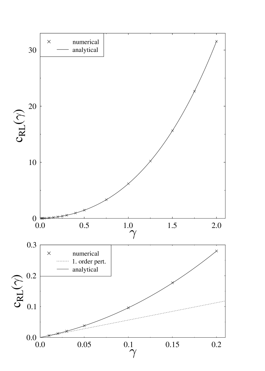
Figure 5: Upper panel: slope parameter $c_{RL}$ of the ‘‘HH fans’’ plotted versus the potential parameter $\gamma$. Crosses: numerical values; solid line: the function $c_{RL}(\gamma)$ given in (35). Lower panel: excerpt for small values of $\gamma$. The dotted line gives the linear approximation to $c_{RL}(\gamma)$, with the slope given in (36), as found in a semiclassical perturbative approach bkwf .

where the negative and positive sign belongs to the R and L type orbits, respectively. At $e=1$ the curves ${\rm tr}\,{\rm M}_{\perp R,L}(e)$ intersect linearly at the two values ${\rm tr}\,{\rm M}_{\perp R,L}(1)=2\mp c_{RL}(\gamma)$, so that the parameter $d$ given above for the standard HH potential is $d=c_{RL}(1)$. The numerical values for $c_{RL}(\gamma)$ are shown by crosses in Fig. 5 below.

The main goal of our paper is to find analytical support for these numerical findings. In Sec. III we will, indeed, confirm the empirical formula (13) analytically in the asymptotic limit $e\to 1$.

III Asymptotic evaluation of stability traces

In this section we derive analytic expressions for ${\rm tr}\,{\rm M}_{\perp}(e)$ of the A, R and L orbits in the GHH system, which are valid in the asymptotic limit $e\to 1$, i.e., close to the barrier. Before presenting them in Sec. III.2 and Sec. III.3, we recall the definitions of the stability matrix ${\rm tr}\,{\rm M}_{\perp}$ and of the monodromy matrix M of which it is a submatrix.

III.1 Monodromy and stability matrices

III.1.1 Stability matrix and the Hill equation

The analytical calculation of the stability matrix ${\rm M}_{\perp}$ of a periodic orbit in a non-integrable system is in general a difficult task. We recall that the stability matrix is obtained from a linearization of the equations of motion and defined by

$$\delta\mbox{{\boldmath$\xi$ \unboldmath}}\!\!_{\perp}(T)={\rm M}_{\perp}\,\delta\mbox{{\boldmath$\xi$ \unboldmath}}\!\!_{\perp}(0)\,,$$ (14)

where $\delta\mbox{{\boldmath$\xi$ \unboldmath}}\!\!_{\perp}(t)$ is the $(2N-2)$-dimensional phase-space vector of infinitesimally small variations transverse to the given periodic orbit ($N$ being the number of independent degrees of freedom), and $T$ is the period of the orbit. For $N=2$ dimensional systems, we may choose $\mbox{{\boldmath$\xi$ \unboldmath}}\!\!_{\perp}(t)=(q,p)$ where $q$ is the coordinate and $p$ the canonical momentum transverse to the orbit in the plane of its motion. $(q,p)$ then form a ‘‘natural’’ canonical pair of Poincaré variables, normalized such that $(q,p)=(0,0)$ is the fixed point of the periodic orbit on the projected Poincaré surface of section (PSS). For two-dimensional Hamiltonians of the form ‘‘kinetic + potential energy’’: $H=T+V$ (and particles with mass $m=1$, so that $p=\dot{q}$), the Newtonian form of the linearized equation of motion for $q(t)$ becomes the Hill equation (see the text book mawi for an explicit discussion)

$${\ddot{q}}(t)+V_{qq}(t)\,q(t)=0\,,$$ (15)

where $V_{qq}(t)$ is the second partial derivative of the potential $V$ with respect to $q$, taken along the periodic orbit, and the two-dimensional stability matrix is given by

$$\left(\begin{array}[]{c}q(T)\\ \dot{q}(T)\end{array}\right)={\rm M}_{\perp}\left(\begin{array}[]{c}q(0)\\ \dot{q}(0)\end{array}\right).$$ (16)

For isolated periodic orbits, solutions of (15) with $q(t)\neq 0$ are in general not periodic. However, when the orbit undergoes a bifurcation, (15) has at least one periodic solution which describes the transverse motion of the new orbit born at the bifurcation; the criterion for the bifurcation to occur is ${\rm tr}\,{\rm M}_{\perp}=+2$ (cf. mawi ).

For particular systems, the Hill equation (15) may become a differential equation with known periodic solutions. For the GHH systems under investigation here, the Hill equation for the A orbit directed along the $y$ axis is given by (3), with $y(t)$ replaced by $y_{A}(t)$ in (6), and becomes the Lamé equation (see, e.g., erde ) whose periodic solutions are the periodic Lamé functions (see lamp for the details). However, the elements of ${\rm M}_{\perp}$ in (16) can in general not be found analytically. One of the rare exceptions is that of the coupled two-dimensional quartic oscillator for which Yoshida yosh derived an analytical expression for ${\rm tr}\,{\rm M}_{\perp}$ as a function of the chaoticity parameter (cf. bfmm ).

Magnus and Winkler mawi have given an iteration scheme for the computation of ${\rm tr}\,{\rm M}_{\perp}$ for periodic orbits in smooth Hamiltonians. We have tried their method for the A orbit in the HH system, but we found mima that its convergence is too slow for computing ${\rm tr}\,{\rm M}_{\perp A}(e)$ with a sufficient accuracy that would allow to deduce the properties of the HH fans. However, in the limit $e\to 1$, it is possible to use an asymptotic expansion of the function ${\rm sn}$ appearing in $y_{A}(t)$ of (6), which allows us to compute ${\rm tr}\,{\rm M}_{\perp A}(e)$ analytically, as discussed in Sec. III.2.

III.1.2 Matrizant and monodromy matrix

For curved periodic orbits – such as the R and L type orbits bifurcating from the A orbit in the GHH systems – which usually can only be found numerically, the phase-space variables $\mbox{{\boldmath$\xi$ \unboldmath}}\!\!_{\perp}$ transverse to the orbit used in the definition (14) of the stability matrix ${\rm M}_{\perp}$ cannot be constructed analytically. Instead, one must in general use Cartesian coordinates and resort to the full monodromy matrix M defined below. For $N=2$, one first linearizes the equations of motion to find the matrizant ${\rm X}(t)$ which propagates small perturbations of the full phase-space vector $\mbox{{\boldmath$\xi$ \unboldmath}}\!\!(t)$ defined by

$$\mbox{{\boldmath$\xi$ \unboldmath}}\!\!(t)=\{x(t),y(t),\dot{x}(t),\dot{y}(t)\}$$ (17)

from their initial values at $t=0$ to a finite time $t$:

$$\delta\mbox{{\boldmath$\xi$ \unboldmath}}\!\!(t)={\rm X}(t)\,\delta\mbox{{\boldmath$\xi$ \unboldmath}}\!\!(0)\,.$$ (18)

For a Hamiltonian of the form $H(x,y,\dot{x},\dot{y})=\frac{1}{2}\,(\dot{x}^{2}+\dot{y}^{2})+V(x,y)$, the differential equation for ${\rm X}(t)$ is

$$\frac{\rm d}{{\rm d}t}\,{\rm X}(t)\;=\;\left(\begin{array}[]{cc}\;\;0&{\rm I}_{2}\\ \!\!-{\rm U}(t)&0\end{array}\right){\rm X}(t)$$ (19)

with the initial conditions

$${\rm X}(0)={\rm I}_{4}\,,$$ (20)

where ${\rm I}_{2}$, ${\rm I}_{4}$ are the two- and four-dimensional unit matrices and U$(t)$ is the two-dimensional Hessian matrix of the potential, taken along the periodic orbit ($po$):

$${\rm U}_{ij}(t)=\frac{\partial^{2}V}{\partial x_{i}\partial x_{j}}\{x(t),y(t)\}_{po}\,,\qquad(x_{i},x_{j}=x,y)\,.$$ (21)

Having solved (19), the monodromy matrix M of the given periodic orbit with period $T$ is defined by

$${\rm M}={\rm X}(T)\,.$$ (22)

In an autonomous system, M has always two unit eigenvalues corresponding small initial variations along the periodic orbit and transverse to the energy shell. After a transformation to an ‘‘intrinsic’’ coordinate system, in which one of the coordinates is always in the direction $r_{\parallel}$ (with momentum $p_{\parallel}=\dot{r}_{\parallel}$) of the periodic orbit gutz , M can be brought into the form

$$M=\left(\begin{array}[]{cc}{\rm M}_{\perp}&{\bf...}\\ {\bf 0}&\left(\begin{array}[]{cc}1&...\\ 0&1\end{array}\right)\end{array}\right),$$ (23)

where the dots denote arbitrary non-zero real numbers and ${\rm M}_{\perp}$ is the stability matrix. The diagonal elements in the lower right block of (23) then correspond to

$${\rm M}_{r_{\parallel}r_{\parallel}}={\rm M}_{\dot{r}_{\parallel}\dot{r}_{\parallel}}=1\,.$$ (24)

The transformation to such an intrinsic coordinate system is quite non-trivial ekwi and not unique. For curved orbits it can in general only be found numerically and is therefore not suitable for analytical calculations. For the curved R and L orbits of our system, we therefore have to resort to the full monodromy matrix M (22) via the solution of (19). For the evaluation of their stability traces, we only need the diagonal elements of M and can then use the obvious relation ${\rm tr}\,{\rm M}_{\perp}={\rm tr}\,{\rm M}-2$.

III.2 Asymptotic evaluation of the stability trace ${\rm tr}\,{\rm M}_{\perp A}(e)$ for $e\to 1$

In the limit $e\to 1$, where the modulus $\kappa$ defined in (8) goes to unity, we may approximate $y_{A}(t)$ by the leading term in the expansion of the function ${\rm sn}(z,\kappa)$ around $\kappa=1$ (see grry )

$${\rm sn}(z,\kappa)\approx{\rm tanh}(z)\,.\qquad(\kappa\to 1)$$ (25)

Since the function $\tanh(z)$ is not periodic, we have to approximate $y_{A}(t)$ in two portions. Taking $t_{2}$ as the time where the orbit passes through its maximum at $y_{2}$, i.e.,

$$y_{A}(t_{2})=y_{2}\quad\Longleftrightarrow\quad t_{2}=[\hbox{\bf K}(\kappa)-F(\varphi,\kappa)]/a_{\kappa}\,,$$ (26)

we define the asymptotic expression for the A orbit over one period by

$${\widetilde{y}}_{A}(t)=\Theta(t_{2}-t)\,Y_{1}(t)+\Theta(t-t_{2})\,Y_{2}(t)\,,\qquad 0\leq t\leq T_{A}\,,$$ (27)

where the functions $Y_{1}(t)$ and $Y_{2}(t)$ are given by

$$Y_{1}(t)=y_{1}+(y_{2}-y_{1})\,\tanh^{2}(z)\,,\qquad Y_{2}(t)=y_{1}+(y_{2}-y_{1})\,\tanh^{2}(z-2\,\hbox{\bf K}(\kappa))\,,$$ (28)

with $z$ given in (7). Although the function (27) is not analytic at $t=t_{2}$, it suffices to find an asymptotic expression for ${\rm tr}\,{\rm M}_{\perp A}(e)$ valid for $e\to 1$.

The details of our calculation are given in Appendix A. The analytical asymptotic result for ${\rm tr}\,{\rm M}_{\perp A}\,(e)$ is given in (70) in terms of associated Legendre functions. In the limit $e\to 1$, the energy dependence of ${\rm tr}\,{\rm M}_{\perp A}\,(e)$ goes only through the period $T_{\rm A}(e)$:

$${\rm tr}\,{\rm M}_{\perp A}\,(e)\;\approx\;{\rm tr}\,{\rm M}_{\perp A}^{(as)}(e)={\rm tr}\,{\rm M}_{\perp A}^{(as)}\,(T_{A}(e),\gamma)\,,\qquad(e\to 1)$$ (29)

where ${\rm tr}\,{\rm M}_{\perp A}^{(as)}\,(T_{A},\gamma)$ is a universal function given by

$${\rm tr}\,{\rm M}_{\perp A}^{(as)}(T_{A},\gamma)=+2\,|\widetilde{F}_{A}(\gamma)|\cos\!\left[\sqrt{1+2\gamma}\,T_{A}-\widetilde{\Phi}_{A}(\gamma)\right]\!.$$ (30)

The phase function $\widetilde{\Phi}_{A}(\gamma)$ is defined through Eqs. (72) and (74), and the amplitude function $|\widetilde{F}_{A}(\gamma)|$ is given explicitly in (75). We recall that $\gamma$ is the potential parameter of the GHH potential (1) is $\gamma=1$ for the standard HH potential. For this case, the result (30) becomes

$${\rm tr}\,{\rm M}_{\perp A}^{(as)}\,(T_{A},1)=2.68043976\,\cos(\!\sqrt{3}\,T_{A}+1.56782696)\,,$$ (31)

where the numerical constants have been calculated for $\gamma=1$. The period of the $\cos$ function in (31) was correctly shown in mbgu to be $2\pi/\!\sqrt{3}$, but the phase $\widetilde{\Phi}_{A}(\gamma=1)$ and the amplitude $2|\widetilde{F}_{A}(\gamma=1)|$ were only obtained numerically. The asymptotic relation (29) had already been observed numerically in davb ; mbgu .

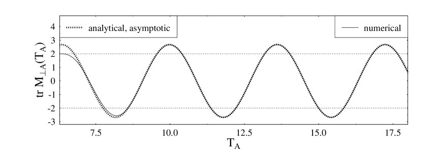
Figure 4: Stability discriminant ${\rm tr}\,{\rm M}_{\perp A}$ of the A orbit in the HH potential ($\gamma=1$), plotted versus period $T_{\rm A}$. Solid line: numerical result (as in Fig. 2, from mbgu ). Dotted line: analytical asymptotic result ${\rm tr}\,{\rm M}_{\perp A}^{(as)}\,(T_{A},1)$ given in (31).

The result (31) is shown in Fig. 4 by the dotted line and compared to the exact numerical result from mbgu , shown by the solid line. We see that the agreement becomes nearly perfect for $T_{\rm A}\,\hbox{\kern 1.00006pt\lower 2.58334pt\hbox{$\sim$} \kern-11.19997pt\raise 2.58334pt\hbox{$>$} }10.5$, corresponding to $e\,\hbox{\kern 1.00006pt\lower 2.58334pt\hbox{$\sim$} \kern-11.19997pt\raise 2.58334pt\hbox{$>$} }e_{6}$. The asymptotic result (29), (30) allows us to give analytical expressions for the bifurcation energies $e_{n}$ in the asymptotic limit $e_{n}\to 1$. The pitchfork bifurcations of the A orbit occur when ${\rm tr}\,{\rm M}_{\perp A}=+2$. We therefore define approximate bifurcation energies $e_{n}^{*}$ by

$${\rm tr}\,{\rm M}_{\perp A}^{(as)}\,(T_{A}(e_{n}^{*}),\gamma)=+2\,.$$ (32)

Using the asymptotic form of $T_{A}(e)$ in (12) and (30), we can give the solutions of (32) in the following formulae

$$e_{2k-1}^{*} \approx 1-432\,\exp\{-[\widetilde{\Phi}_{A}(\gamma)-\arccos(1/|\widetilde{F}_{A}(\gamma)|)+2\pi k]/\!\sqrt{1+2\gamma}\},\qquad(\hbox{R})$$

$$e_{2k}^{*} \approx 1-432\,\exp\{-[\widetilde{\Phi}_{A}(\gamma)+\arccos(1/|\widetilde{F}_{A}(\gamma)|)+2\pi k]/\!\sqrt{1+2\gamma}\},\qquad(\hbox{L})$$ (33)

where $k=3,4,5,\dots$, and the odd numbers $n=2k-1$ refer to the R type and even $n=2k$ to the L type bifurcations, respectively. For $e_{n}^{*}$ sufficiently close to 1, i.e., for large enough $n$ the above values should reproduce the numerically obtained ‘‘exact’’ values $e_{n}$.

This is demonstrated for $\gamma=1$ in Tab. 1. In the second column we give the resulting values of $e_{n}^{*}$ with $5\leq n\leq 16$ for the standard HH system, and in the third column we reproduce their numerical values $e_{n}$ obtained in lamp as roots of the equation ${\rm tr}\,{\rm M}_{\perp A}(e_{n})=+2$. As we see, the asymptotic results $e_{n}^{*}$ approach the numerical values $e_{n}$ very well already starting from $n=7$, as could be expected from Fig. 4. In view of the numerical difficulties in determining the $e_{n}$ from a search of periodic orbits (cf. the remarks after Fig. 3), the agreement is very satisfactory for all $n\geq 7$.

This is in itself a remarkable result, because we are not aware of any analytical results for bifurcation energies (or bifurcation values of any chaoticity parameter) in non-integrable Hamiltonian systems, except for the coupled two-dimensional quartic oscillator (see lamp ; bfmm ). In the present case, the bifurcation energies $e_{n}$ can be related to the eigenvalues of the Lamé equation. These can, in principle, be given by infinite continued fractions inc1 , but their determination is hereby only possible numerically by iteration, which becomes even less accurate than the numerical solution of ${\rm tr}\,{\rm M}_{\perp A}(e_{n})=+2$ as done in lamp . The analytical expressions (33) therefore represent an important achievement of this paper.

III.3 Asymptotic evaluation of ${\rm tr}\,{\rm M}_{\perp R,L}(e)$ for $e\to 1$

For the stability traces of the R and L orbits we need, as mentioned in Sec. III.1.2 above, to know the diagonal elements of the full monodromy matrix M, i.e., the elements X${}_{ii}(t=T)$ with $i=x,y,\dot{x},\dot{y}$. Since the equations (19) couple all 16 elements of X$(t)$, this is still a considerable task. It can, however, be simplified considerably in the asymptotic limit $e\to 1$. First, we can make use of the ‘‘frozen $y$ motion approximation’’ (in short: ‘‘frozen approximation’’, FA) introduced in Refs. mbgu ; lamp . It exploits the fact that near the bifurcation energies $e_{n}$ at which the R and L orbits are born, their motion in the $y$ direction is close to that of the bifurcating A orbit and, for increasing energy $e$, changes only very little. It can be shown (cf. bfmm and Sec. IV below) that this may correspond to the first order in a perturbative expansion in the parameter $e-e_{n}$, valid to leading order in the small quantity $1-e_{n}$. Second, we can exploit some symmetry relations between the elements of M if the initial point at $t=0$ for the calculation of X$(t)$ is chosen as the upper turning point in the direction of the A orbit, i.e., its maximum along the $y$ axis. These symmetry relations are derived in Sec. B.1; their main consequence is that we only need to calculate the 4$\times$4 submatrix of X${}_{ij}(t)$ with spatial indices $i,j=x,y$, and that we have the asymptotic equality ${\rm tr}\,{\rm M}_{\perp R,L}\approx 2$M_yy for $e\to 1$, see (98). As shown below, these symmetry relations can be used also beyond the FA, and only in order to simplify them some properties of the FA will be exploited in our further derivations.

With these approximations, the calculation of ${\rm tr}\,{\rm M}_{\perp R,L}(e)$ proceeds similarly as that of ${\rm tr}\,{\rm M}_{\perp A}(e)$ discussed in the previous section; its details are presented in Appendix B. The analytical result is given in (121) in terms of associated Legendre functions. After their expansion in the asymptotic limit $e\to 1$ we obtain the result

$${\rm tr}\,{\rm M}_{\perp R,L}^{(as)}(e)\;=\;2\mp c_{RL}(\gamma)\,\frac{(e-e_{n})}{(1-e_{n})}\,,\qquad(e\geq e_{n}\to 1)$$ (34)

where the ‘‘$-$’’ and ‘‘$+$’’ sign belongs to the R and L orbits, respectively. The slope function $c_{RL}(\gamma)$ is found analytically to be

$$c_{RL}(\gamma)=\frac{4\sqrt{1+2\gamma}}{\sinh[2\pi\sqrt{1+2\gamma}]}\cosh\left(\frac{\pi}{2}\sqrt{48\gamma-1}\right).$$ (35)

Eq. (34) has exactly the functional structure of the empirical ‘‘GHH fan’’ formula (13). Mathematically, it holds asymptotically in the limit $e_{n}\to 1$ to leading order in the small parameter $\sqrt{1-e_{n}}$. We emphasize that this result confirms also the numerical finding that, for large enough $n$ (practically, for $n>8$) the functions ${\rm tr}\,{\rm M}_{\perp R,L}(e)$ are linear in $e$ from $e_{n}$ up to at least $e=1$.

In Fig. 5 we show by crosses the values of $c_{RL}(\gamma)$, evaluated numerically from the stability of the R and L orbits at $e=1$, as a function of $\gamma$. The solid line shows the analytical result (35). In the lower part of the figure, we show the region of small $\gamma$. The curve $c_{RL}(\gamma)$ goes through zero with a finite slope which can easily be found by Taylor expanding (35) after the replacement $\cosh{(\pi\sqrt{48\gamma-1}/2)}\rightarrow\cos{(\pi\sqrt{1-48\gamma}/2)}$. The slope at $\gamma=0$ becomes

$$c^{\prime}_{\!RL}(0)=\left.\frac{{\rm d}}{{\rm d}\gamma}\,c_{RL}(\gamma)\right|_{\gamma=0}=\frac{48\pi}{\sinh{(2\pi)}}=0.56320942\,.$$ (36)

This value is found analytically bkwf from a semiclassical perturbative approach, in which the term $\gamma\,x^{2}y$ of the Hamiltonian (1) is treated as a perturbation. Using the perturbative trace formula given by Creagh crea one can extract the stabilities of the R and L orbits which in this approach are created from the destruction of rational tori (see bkwf for details). To first order in the perturbation, one obtains exactly the correct linear approximation to $c_{RL}(\gamma)$, with the slope (36), shown in the lower part of Fig. 5 by the dotted line note .

The theoretical value of $c_{RL}(1)=6.18199717$ agrees very well with the value $d=6.183\pm 0.001$ that was found from the numerical stabilities of the R_n and L${}_{n^{\prime}}$ orbits in the standard HH potential ($\gamma=1$) for $9\leq n,n^{\prime}\leq 13$, evaluated at $e=1$.

Our result (34) obeys a known ‘‘slope theorem’’ for pitchfork bifurcations bttb ; ssun ; jaen1 . It states that the slope of ${\rm tr}\,{\rm M}_{\perp}(e)$ of the new orbits born at the bifurcation point $e_{n}$ equals minus twice that of the parent orbit. Specifically in the present system, it says

$$\frac{{\rm d}}{{\rm d}e}\,{\rm tr}\,{\rm M}_{\perp R,L}(e_{n})=-2\,\frac{{\rm d}}{{\rm d}e}\,{\rm tr}\,{\rm M}_{\perp A}(e_{n})\,.$$ (37)

We can easily obtain the slopes of ${\rm tr}\,{\rm M}_{\perp A}(e)$ at $e=e_{n}$ from the asymptotic result for ${\rm tr}\,{\rm M}_{\perp A}^{(as)}(e)$ given in (30). By its Taylor expansion around the asymptotic bifurcation energy $e_{n}^{*}$ given by (33), we find up to first order in $e-e_{n}^{*}$

$${\rm tr}\,{\rm M}_{\perp A}^{(as)}(e)=2\pm c_{A}(\gamma)\,\frac{(e-e_{n}^{*})}{(1-e_{n}^{*})}+{\cal O}\left[\frac{(e-e_{n}^{*})^{2}}{(1-e_{n}^{*})^{3/2}}\right]\,.$$ (38)

The alternating sign of the linear term is ‘‘$+$’’ for the R and ‘‘$-$’’ for the L type orbit bifurcations and thus opposite to that in (34). The slope function $c_{A}(\gamma)$ is found to be

$$c_{A}(\gamma)=\left|\frac{{\rm d}}{{\rm d}T_{A}}{\rm tr}\,{\rm M}_{\perp A}^{(as)}(T_{A},\gamma)\right|_{T_{A}=\widetilde{T}_{A}(e_{n}^{*})}\!\!\! = 2\sqrt{1+2\gamma}\sqrt{|\widetilde{F}_{A}(\gamma)|^{2}-1}$$ (39)

$$= \frac{2\sqrt{1+2\gamma}}{\sinh[2\pi\sqrt{1+2\gamma}]}\cosh\left(\frac{\pi}{2}\sqrt{48\gamma-1}\right),$$

where $|\widetilde{F}_{A}(\gamma)|$ is given in (75) and $\widetilde{T}_{A}(e)$ in (12). Note that $c_{A}(\gamma)$ does not depend on the bifurcation energy $e_{n}^{*}$ since ${\rm tr}\,{\rm M}_{\perp A}^{(as)}\,(T_{A},\gamma)$ is a periodic function of $T_{A}$. Comparing Eqs. (35) and (39), we see that $c_{RL}(\gamma)=2c_{A}(\gamma)$ so that the theorem (37) is, indeed, fulfilled with the correct sign.

IV Perturbative evaluation of ${\rm tr}\,{\rm M}_{\perp R,L}(e)$ near $e=1$

Here we present an iterative perturbative approach for the calculation of the stability trace of the new orbits born at the bifurcation energies $e_{n}$ of the A orbit for the GHH Hamiltonian (1), taking R orbits as example. This approach can be useful for Hamiltonians for which we do not find symmetry properties like those given in (92) and (93), which allowed for a non-perturbative calculation of the stability traces.

As the small perturbation parameter we introduce the available energy above the bifurcation point

$$\epsilon=e-e_{n}\,,$$ (40)

which is always positive. The $x$ and $y$ coordinates of the new orbits, labeled $x_{po}$ and $y_{po}$, and the relevant elements of their monodromy matrices, all as functions of time $t$, can be expanded in powers of small perturbation parameter $\epsilon$:

$$y_{po}(t) = y_{A}(t)+\epsilon\,{y}_{po}^{(1)}(t)+\ldots,\qquad\;x_{po}(t)=u_{po}\!\left[{x}_{po}^{(0)}(t)+\epsilon\,{x}_{po}^{(1)}(t)+\ldots\right],$$ (41)

$${\rm X}_{ii}(t) = {{\rm X}}_{ii}^{(0)}(t)+\epsilon\,{{\rm X}}_{ii}^{(1)}(t)+\ldots\,,\quad\;{\rm X}_{ij}(t)=u_{po}\!\left[{{\rm X}}_{ij}^{(0)}(t)+\epsilon\,{{\rm X}}_{ij}^{(1)}(t)+\ldots\right]\;(i\neq j)\,,\leavevmode\nobreak\ \leavevmode\nobreak\ \leavevmode\nobreak\$$ (42)

where $i,j=x,y$. The superscripts ^(m) indicate in an obvious manner the power $\epsilon^{m}$ at which the corresponding terms appear at the $m$-th order of the expansion. The normalization constants $u_{po}$ of $x_{po}(t)$ are given by

$$u_{R}=\sqrt{\frac{e-e_{n}}{3}}\,,\qquad u_{L}=\sqrt{\frac{e-e_{n}}{3(1+2\gamma y_{2})}}\,.$$ (43)

Note that they both are proportional to $\sqrt{\epsilon}$, so that $x_{po}(t)$ goes to zero in the limit $e\to e_{n}$. The solution of the equations (96) with the initial conditions (B.1.3) for the stability trace ${\rm tr}\,{\rm M}_{\perp R,L}(e)$ using the perturbative expansions (41) and (42) is presented in the Appendix C for the case of the R type orbits. The calculation for the L type orbits is completely analogous. The asymptotic result for ${\rm tr}\,{\rm M}_{\perp R}(e)$ is given in (131).

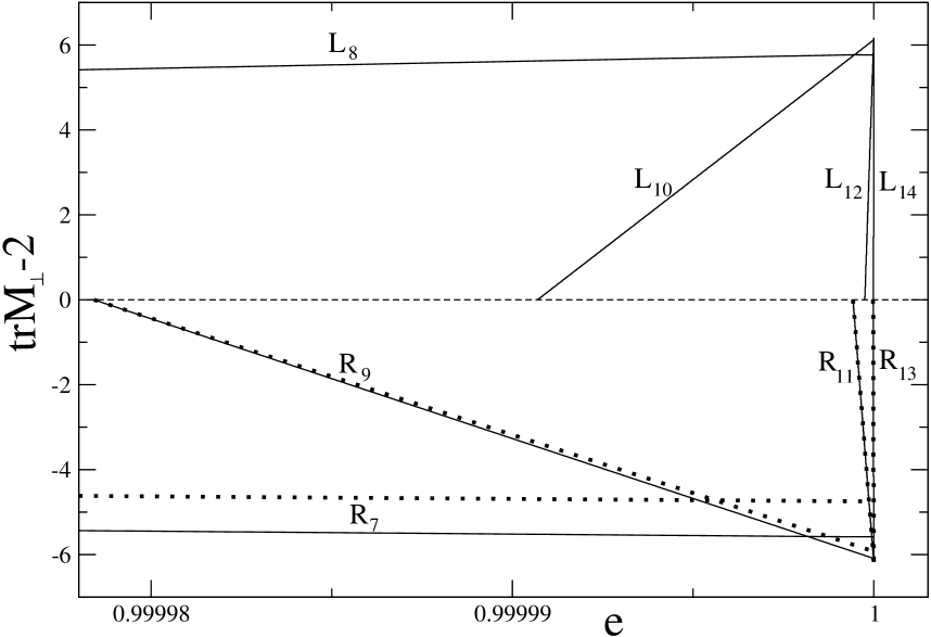
Figure 6: Stability traces $\,{\rm tr}\,{\rm M}_{\perp R,L}-2\,$ as functions of the energy $e$ at $\gamma=1$. Solid lines show the analytical expression (B.2) for $R_{n}$ and $L_{n}$ orbits with $n=7-14$. Dashed lines are the perturbative results (131) for a few R orbits as examples.

We now compare the non-perturbative result (B.2) and the perturbative approximation (131) for the stability traces ${\rm tr}\,{\rm M}_{\perp R,L}(e)$ with numerical results. Fig. 6 shows by solid lines the asymptotic analytical results (B.2) for the case $\gamma=1$. They form the ‘‘HH fans’’ with their linear energy dependence of ${\rm tr}\,{\rm M}_{\perp R,L}(e)$ around $e=1$, intersecting at the values ${\rm tr}\,{\rm M}_{\perp R,L}(1)-2=\mp c_{RL}(1)$ with $c_{RL}(1)\approx 6.182$ for the R and L type orbits, respectively. As seen from this figure, they become approximately symmetric with respect to the line ${\rm tr}\,{\rm M}_{\perp}=+2$, starting from $n=9$ in good agreement with the numerical results lamp . Note that the linear dependence of ${\rm tr}\,{\rm M}_{\perp R,L}(e)$ (B.2) is obtained up to terms of relative order $\sqrt{1-e_{n}}$. The perturbative result for the R type orbits (131) is shown by the dashed lines, in good agreement with the analytical result (B.2) already for $n\geq 9$.

For further comparison with numerical results, we define the ‘‘slope parameter’’

$$d_{n}=|{\rm tr}\,{\rm M}_{\perp R,L}(e=1)-2|\,,$$ (44)

evaluating ${\rm tr}\,{\rm M}_{\perp R,L}$ at the barrier ($e=1$) for a given orbit $R_{n}$ or $L_{n}$ born at the bifurcation energy $e_{n}$. As shown in Sec. III.3 and Appendix B.2, this parameter tends to the asymptotic limit $c_{RL}(\gamma)$, given in (35), for $n\to\infty$.

Tab. 2 shows the slope parameter $d_{n}$ (44) for $7\leq n\leq 20$, evaluated for $\gamma=1$ in various approximations; in the left part for R type orbits (odd $n$) and in the right part for L type orbits (even $n$). $d_{n}^{an}$ in columns 3 and 7 are the non-perturbative analytical results from (B.2), $d_{n}^{sa}$ in column 2 represents the perturbative semi-analytical result (131) for the R orbits, and $d_{n}^{num}$ in columns 5 and 9 are the numerical results lamp . Columns 4 and 8 contain $d_{n}^{num*}$ obtained numerically from solving the equations of motion (3) and (4) for the periodic orbits with using the FA initial conditions (87) and (94) at the top turning point (76), and Eqs. (19) at $t=T$ for the monodromy matrix elements. This approximation is in good agreement with the full numerical results for large enough $n$, the better the larger $n$, as seen from comparison of the 4th and 5th (and the last two) columns in Tab. 2. The bifurcation energies for $n\geq 12$ were taken analytically from Tab. 1. For smaller $n$, they were obtained by numerically solving equation ${\rm tr}\,{\rm M}_{\perp A}(e_{n})=2$ with a precision better than $|{\rm tr}\,{\rm M}_{\perp A}(e_{n})-2|\,\hbox{\kern 1.00006pt\lower 2.58334pt\hbox{$\sim$} \kern-11.19997pt\raise 2.58334pt\hbox{$<$} }10^{-9}$. As seen from this Table, one has good agreement of the asymptotic behavior of $d_{n}$ of the perturbative $d_{n}^{sa}$ and even better analytical results $d_{n}^{an}$ as compared with these numerical calculations. It should be noted also that the slope parameter (44) of the perturbative approach (131) within the FA, see (122), even without the correction (125) to the periodic orbit $y_{A}(t)$, is in rather good agreement with the numerical results presented in Tab. 2, especially for asymptotically large $n$, with a precision better than 5%. However, the second correction in (131) above the FA improves essentially the slope parameter (44) in this asymptotic region. As noted above, the asymptotic values of the perturbative $d_{n}^{sa}$ and the non-perturbative $d_{n}^{an}$, as well as the numerical FA result for $d_{n}^{num*}$, all converge sufficiently rapidly to the asymptotic analytical number $c_{RL}(1)=6.18199717$ given by Eq. (35), in line with the analytical convergence found above from (121).

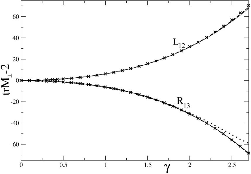
Figure 7: Stability traces ${\rm tr}\,{\rm M}_{\perp R,L}-2$ as functions of $\gamma$ for R and L orbits, respectively, evaluated at the barrier energy $e=1$. Solid lines show the analytical expression (B.2) for the orbits $R_{13}$ and $L_{12}$; dashed lines the asymptotic results (35) for $\mp c_{RL}(\gamma)$; dots are the perturbative results to (131); and crosses show the numerical results $\mp d_{n}^{num*}$ with the FA initial conditions as in Tab. 2. The bifurcation energies $e_{n}(\gamma)$ are obtained analytically through Eqs. (33).

Fig. 7 shows good agreement between the analytical (B.2), semi-analytical (131) and numerical solving the GHH equations (3), and (4) for classical periodic orbits and (19) for the monodromy matrix with FA initial conditions for $L_{12}$ and $R_{13}$ as examples. Both these curves agree very well with the asymptotic analytical slopes $c_{RL}(\gamma)$ within a rather wide interval of $\gamma$ even for not too large $n$ of the orbits mentioned above. This comparison is improved with increasing $n$, the better the larger $n$, which gives a numerical confirmation of the analytical convergence of the ${\rm tr}\,{\rm M}_{\perp R,L}(e,\gamma)$ (B.2) to the asymptotic $c_{RL}(\gamma)$ (35) at the barrier $e=1$ for any $\gamma$. For larger $\gamma$, one needs larger $n$ in order to obtain convergence of all the compared curves.

V Summary and conclusions

In this paper we have investigated the bifurcation cascades of the linear A orbit in a class of generalized Hénon-Heiles (GHH) potentials. We were able to derive analytical expressions for the stability traces ${\rm tr}\,{\rm M}_{\perp A}(e)$ of the A orbit and ${\rm tr}\,{\rm M}_{\perp R,L}(e)$ of the R and L orbits bifurcating from it as functions of the energy, which are asymptotically valid for energies close to the saddle at $e=1$, i.e., in the limit where the bifurcations energies $e_{n}$ approach the saddle: $e_{n}\to 1$. Our results confirm analytically the empirical numerical properties of the ‘‘Hénon-Heiles fans’’ that are formed by the asymptotically linear intersection of the functions ${\rm tr}\,{\rm M}_{\perp R,L}(e)$ at $e=1$, as given in Eq. (34). We found good agreement of our alternative non-perturbative and perturbative asymptotic results for ${\rm tr}\,{\rm M}_{\perp R,L}(e)$ with the numerical results. As a bonus, we have also obtained asymptotically exact expressions for the bifurcation energies $e_{n}$ of the A orbit in the GHH system, given in Eq. (33). Our results can be interpreted in the sense that the non-integrable, chaotic GHH Hamiltonian becomes approximately integrable locally at the barrier, i.e., for $e=1$.

Both our approaches may be useful, also for more general Hamiltonians, for semiclassical calculations of the Gutzwiller trace formula for the level density gutz , extended to bifurcation cascades with the help of suitable normal forms and corresponding uniform approximations ozob ; ssun . A normal form with uniform approximation for two successive pitchfork bifurcations has been derived and successfully applied to the HH system in jkmb . In future research, we hope to generalize the normal form theory to infinitely dense bifurcation sequences with the help of the results of maf ; jkmb and the theory of Fedoryuk fedorpr ; fedorbook . Hereby the ‘‘HH fan’’ phenomenon for the stability traces might be useful.

Appendix A Asymptotic evaluation of ${\rm tr}\,{\rm M}_{\perp A}(e)$ for $e\to 1$

To obtain the stability matrix ${\rm M}_{\perp A}$ for the orbit A, we have to solve the linearized equation of motion (15) for small perturbations around the orbit in the perpendicular direction. Since the A orbit moves along the $y$ axis, we have $q=x$, $p=\dot{x}$ and (15) becomes (3) which is already linear in $x$. We thus find ${\rm M}_{\perp A}$ from the non-periodic solutions of (3) with small initial values $x_{0}=x(t=0)$, ${\dot{x}}_{0}={\dot{x}}(t=0)$. Let us denote these solutions by $x(t;x_{0},{\dot{x}}_{0})$. The elements of ${\rm M}_{\perp A}$ (we omit the subscript ‘‘$\perp$A’’ for simplicity) are then given by

$${\rm M}_{qq}=\lim_{x_{0}\to 0}{\frac{x(T_{A};x_{0},0)}{x_{0}}}\,,\qquad{\rm M}_{qp}=\lim_{\dot{x}_{0}\to 0}{\frac{x(T_{A};0,\dot{x}_{0})}{\dot{x}_{0}}}\,,$$ (45)

$${\rm M}_{pq}=\lim_{x_{0}\to 0}{\frac{\dot{x}(T_{A};x_{0},0)}{x_{0}}}\,,\qquad{\rm M}_{pp}=\lim_{\dot{x}_{0}\to 0}{\frac{\dot{x}(T_{A};0,\dot{x}_{0})}{\dot{x}_{0}}}\,.$$ (46)

We could not find exact analytical solutions of (3) using the exact function $y_{A}(t)$ (6) for the A orbit, for which (3) becomes the Lamé equation. Only at the bifurcation energies $e_{n}$, one of its solutions is a periodic Lamé function which has known expansions erde . For the non-periodic solutions, no expansions could be found in the literature. We can, however, solve (3) if we instead of the exact $y_{A}(t)$ use the approximation ${\tilde{y}}_{A}(t)$ given in (27), which becomes exact in the asymptotic limit $e\to 1$, and for which (3) can be reduced to the Legendre equation as shown below. We proceed separately for the two time intervals $0\leq t\leq t_{2}$ and $t_{2}\leq t\leq T_{A}$, as specified after (25):

a) $0\leq t\leq t_{2}$: Solve the equation

$$\ddot{x}_{1}(t)+[1+2\gamma Y_{1}(t)]\,x_{1}(t)=0\,,$$ (47)

with the initial conditions

$$x_{1}(0)=x_{0}=0\,,\qquad\dot{x}_{1}(0)=\dot{x}_{0}\to 0\,,$$ (48)

and obtain $x_{1}(t_{2})$.

b) $t_{2}\leq t\leq T_{A}$: Solve the equation

$$\ddot{x}_{2}(t)+[1+2\gamma Y_{2}(t)]\,x_{2}(t)=0\,,$$ (49)

with the initial conditions

$$x_{2}(t_{2})=x_{1}(t_{2})\,,\qquad\dot{x}_{2}(t_{2})=\dot{x}_{1}(t_{2})\,,$$ (50)

and obtain $x_{2}(T_{A})$.

To do so, we transform equations (47), (49) by defining the following variables:

$$z_{1}=z\,,\qquad z_{2}=z-2\,\hbox{\bf K}(\kappa)\,.$$ (51)

Then, the equations (47), (49) can be written compactly as:

$$\frac{{\rm d}^{2}}{{\rm d}z^{2}}x_{i}(z_{i})+[B+A\tanh^{2}(z_{i})]\,x_{i}(z_{i})=0\,,\qquad(i=1,2)$$ (52)

where

$$B=\frac{6(1+2\gamma y_{1})}{(y_{3}-y_{1})}\,,\qquad A=\frac{12\gamma(y_{2}-y_{1})}{(y_{3}-y_{1})}\,.$$ (53)

We next go over to the new variables

$$s_{i}=\tanh(z_{i})\,.\qquad(i=1,2)$$ (54)

Then (52) is transformed into the Legendre equation:

$$(1-s_{i}^{2})\,\frac{{\rm d}^{2}}{{\rm d}s^{2}}x_{i}(s_{i})-2s_{i}\,\frac{{\rm d}}{{\rm d}s}x_{i}(s_{i})+\left[\nu(\nu+1)-\frac{\mu^{2}}{1-s^{2}_{i}}\right]\!x_{i}(s_{i})=0\,,\qquad(i=1,2)$$ (55)

with

$$\mu=i\sqrt{A+B}\,,\qquad\nu=(-1+i\sqrt{4A-1})/2\,.$$ (56)

The Legendre equation (55) has the solution

$${x}_{i}(s_{i})=C_{1i}P_{\nu}^{\mu}(s_{i})+C_{2i}Q_{\nu}^{\mu}(s_{i})\,,\qquad(i=1,2),$$ (57)

where $P_{\nu}^{\mu}(s)$ and $Q_{\nu}^{\mu}(s)$ are the associated Legendre functions of first and second kind, respectively, with real argument $-1\leq s\leq+1$ (see grry ). The initial conditions (50) for $x_{2}(s_{2})$ have the form

$$x_{2}(-s_{K})=x_{1}(s_{K})\,,\qquad\quad\Bigl{(}\frac{{\rm d}x_{2}(s_{2})}{{\rm d}s_{2}}\Bigr{)}_{s_{2}=-s_{K}}=\Bigl{(}\frac{{\rm d}x_{1}(s_{1})}{{\rm d}s_{1}}\Bigr{)}_{s_{1}=s_{K}}\,,$$ (58)

where

$$s_{K}=\tanh\hbox{\bf K}(\kappa)=\tanh(a_{\kappa}T_{A}/2)\,.$$ (59)

Solution (57) of equation (55) for $i=1$ with the initial conditions (48) yields the following expressions for the coefficients $C_{11}$ and $C_{21}$:

$$C_{11}=\dot{x}_{0}\,D^{\mu}_{\nu}(s_{F})\,Q^{\mu}_{\nu}(s_{F})\,,\qquad C_{21}=-\dot{x}_{0}\,D^{\mu}_{\nu}(s_{F})\,P^{\mu}_{\nu}(s_{F})\,,$$ (60)

with

$$s_{F}=\tanh F(\varphi,\kappa)\,,\qquad D^{\mu}_{\nu}(s_{F})=\left[a_{\kappa}(1-s_{F}^{2})\,W_{\nu}^{\mu}(s_{F})\right]^{-1}.$$ (61)

Here $W_{\nu}^{\mu}(s_{F})$ is the Wronskian

$$W_{\nu}^{\mu}(s)\equiv W\{Q^{\mu}_{\nu}(s),P^{\mu}_{\nu}(s)\}=Q^{\mu}_{\nu}(s)\frac{{\rm d}}{{\rm d}s}{P^{\mu}_{\nu}}(s)-P^{\mu}_{\nu}(s)\frac{{\rm d}}{{\rm d}s}{Q^{\mu}_{\nu}}(s)\,.$$ (62)

Analogously, we solve equation (55) for $i=2$ with the initial conditions (58) and obtain for $C_{12}$ and $C_{22}$ the following expressions:

$$C_{12}=\dot{x}_{0}\,D^{\mu}_{\nu}(s_{F})\,\frac{a_{1}Q^{\mu}_{\nu}(s_{F})+a_{2}P^{\mu}_{\nu}(s_{F})}{W_{\nu}^{\mu}(s_{K})}\,,$$ (63)

$$C_{22}=\dot{x}_{0}\,D^{\mu}_{\nu}(s_{F})\,\frac{a_{3}Q^{\mu}_{\nu}(s_{F})+a_{4}P^{\mu}_{\nu}(s_{F})}{W_{\nu}^{\mu}(s_{K})}\,.$$ (64)

The coefficients $a_{i}$ here are:

$$a_{1}=Q^{\mu}_{\nu}(-s_{K})\frac{{\rm d}}{{\rm d}s}{P^{\mu}_{\nu}}(s_{K})-P^{\mu}_{\nu}(s_{K})\frac{{\rm d}}{{\rm d}s}{Q^{\mu}_{\nu}}(-s_{K})\,,$$

$$a_{2}=Q^{\mu}_{\nu}(s_{K})\frac{{\rm d}}{{\rm d}s}{Q^{\mu}_{\nu}}(-s_{K})-Q^{\mu}_{\nu}(-s_{K})\frac{{\rm d}}{{\rm d}s}{Q^{\mu}_{\nu}}(s_{K})\,,$$

$$a_{3}=P^{\mu}_{\nu}(s_{K})\frac{{\rm d}}{{\rm d}s}{P^{\mu}_{\nu}}(-s_{K})-P^{\mu}_{\nu}(-s_{K})\frac{{\rm d}}{{\rm d}s}{P^{\mu}_{\nu}}(s_{K})\,,$$

$$a_{4}=P^{\mu}_{\nu}(-s_{K})\frac{{\rm d}}{{\rm d}s}{Q^{\mu}_{\nu}}(s_{K})-Q^{\mu}_{\nu}(s_{K})\frac{{\rm d}}{{\rm d}s}{P^{\mu}_{\nu}}(-s_{K})\,.$$ (65)

Using $x_{2}$ in (57) at $t=T_{A}$ and (63), (64) for the coefficients $C_{12}$, $C_{22}$, we obtain the following expression for ${\rm M}_{pp}$ defined in (46):

$${\rm M}_{pp} = \left[W_{\nu}^{\mu}(s_{F})W_{\nu}^{\mu}(s_{K})\right]^{-1}\left[a_{1}Q^{\mu}_{\nu}(s_{F})\frac{{\rm d}}{{\rm d}s}{P^{\mu}_{\nu}}(s_{F})+a_{2}P^{\mu}_{\nu}(s_{F})\frac{{\rm d}}{{\rm d}s}{P^{\mu}_{\nu}}(s_{F})\right.$$ (66)

$$+ \left.a_{3}Q^{\mu}_{\nu}(s_{F})\frac{{\rm d}}{{\rm d}s}{Q^{\mu}_{\nu}}(s_{F})+a_{4}P^{\mu}_{\nu}(s_{F})\frac{{\rm d}}{{\rm d}s}{Q^{\mu}_{\nu}}(s_{F})\right].$$

To calculate ${\rm M}_{qq}$ defined in (45), we solve equations (47), (49) with the initial conditions

$$x_{1}(0)=x_{0}\to 0\,,\qquad\dot{x}_{1}(0)=\dot{x}_{0}=0\,,$$ (67)

and then take into account the condition (50). Using the same steps as for ${\rm M}_{pp}$, we obtain ${\rm M}_{qq}$ in the following form:

$${\rm M}_{qq} = -\left[W_{\nu}^{\mu}(s_{F})W_{\nu}^{\mu}(s_{K})\right]^{-1}\left[a_{1}P^{\mu}_{\nu}(s_{F})\frac{{\rm d}}{{\rm d}s}{Q^{\mu}_{\nu}}(s_{F})+a_{2}P^{\mu}_{\nu}(s_{F})\frac{{\rm d}}{{\rm d}s}{P^{\mu}_{\nu}}(s_{F})\right.$$ (68)

$$+ \left.a_{3}Q^{\mu}_{\nu}(s_{F})\frac{{\rm d}}{{\rm d}s}{Q^{\mu}_{\nu}}(s_{F})+a_{4}Q^{\mu}_{\nu}(s_{F})\frac{{\rm d}}{{\rm d}s}{P^{\mu}_{\nu}}(s_{F})\right].$$

Using the following explicit expression for the Wronskian (62),

$$W^{\mu}_{\nu}(s)=\frac{1}{(s^{2}-1)}\frac{\Gamma(1+\nu+\mu)}{\Gamma(1+\nu-\mu)}\,,$$ (69)

we now find for the sum of ${\rm M}_{qq}$ and ${\rm M}_{pp}$

$${\rm tr}\,{\rm M}_{\perp A}(e)=2\,(s_{K}^{2}-1)\,\frac{\Gamma(1+\nu-\mu)}{\Gamma(1+\nu+\mu)}\left[Q^{\mu}_{\nu}(-s_{K})\frac{{\rm d}}{{\rm d}s}{P^{\mu}_{\nu}}(s_{K})-P^{\mu}_{\nu}(-s_{K})\frac{{\rm d}}{{\rm d}s}{Q^{\mu}_{\nu}}(s_{K})\right]\!.$$ (70)

Note that the energy dependence comes through the quantities $\mu$, $\nu$ given in (56) and $s_{K}$ in (59) via the turning points $y_{i}(e)$ given in (9). As must be expected, the result (70) does not depend on the initial point $y_{0}$.

We recall that the result (70) has been obtained using the approximation (27) for the function $y_{A}(t)$, which is based on the asymptotic expression (25) for the Jacobi elliptic function sn$(z,\kappa)$, valid in the limit $\kappa\to 1$. We can therefore simplify the above result by taking asymptotic limits, valid for $e\to 1$, of the quantities appearing in (70). Since we have omitted the next-to-leading correction to (25), it is consistent to keep only the leading asymptotic terms. (An evaluation of all next-to-leading order corrections would lead outside the scope of this paper.)

Using the asymptotic forms of the Legendre functions through hypergeometric series (cf. grry , Eqs. 8.704, 8.705, and 8.737), we obtain for the leading term in (70) the intermediate result

$${\rm tr}\,{\rm M}_{\perp A}(e)\approx 2\,{\rm Re}\left(e^{-a_{\kappa}T_{A}\mu}F_{A}\right),$$ (71)

where the function $F_{A}(\gamma)$ is defined by

$$F_{A}(\gamma)=\frac{\mu\pi}{\sin^{2}(\mu\pi)}\,\frac{\Gamma(1+\nu+\mu)\,\sin[(\nu+\mu)\pi]}{\Gamma(1+\nu-\mu)\,\Gamma^{2}(1+\mu)}=|F_{A}(\gamma)|\,e^{i\Phi_{A}(\gamma)}\,.$$ (72)

Here the period $T_{A}$ and the quantities $a_{\kappa}$ in (8), and $\mu,\nu$ given in (56) still depend on the energy $e$. Now, for $e\to 1$, all quantities in (71) except $T_{A}(e)$ have finite limits, easily found from the limiting turning points $y_{1}\to-1/2$, $y_{2}\to 1$, $y_{3}\to 1$. In particular, we get the limits:

$$a_{\kappa}\to 1/2\,,\quad\mu\to 2i\sqrt{1+2\gamma}\,,\quad\nu\to\frac{1}{2}\left(-1+i\sqrt{48\gamma-1}\right).\qquad(e\to 1)$$ (73)

The limit of $F_{A}(\gamma)$ will be denoted by $\widetilde{F}_{A}(\gamma)$ and its limiting phase by $\widetilde{\Phi}_{A}(\gamma)$

$$F_{A}(\gamma)\;\to\;\widetilde{F}_{A}(\gamma)=|\widetilde{F}_{A}(\gamma)|\,e^{i\widetilde{\Phi}_{A}(\gamma)}\,.\qquad(e\to 1)$$ (74)

Its modulus can be given analytically as

$$|\widetilde{F}_{A}(\gamma)|=\frac{\sqrt{\cosh(4\pi\sqrt{1+2\gamma})+\cosh(\pi\sqrt{48\gamma-1})}}{\sqrt{2}\,\sinh[2\pi\sqrt{1+2\gamma}]}.$$ (75)

We discuss only positive values of $\gamma$ here; for $\gamma<1/48$, the function $\cosh{(\pi\sqrt{48\gamma-1})}$ becomes equal to $\cos{(\pi\sqrt{1-48\gamma})}$. The phase $\widetilde{\Phi}_{A}(\gamma)$ is defined through Eqs. (72) and (74); it turns out to be negative for all $\gamma>0$.

Using the above limits, we finally get from (71) the asymptotic expression for ${\rm tr}\,{\rm M}_{\perp A}(e)$ given in Eqs. (29) and (30) of Sec. III.

Appendix B Asymptotic evaluation of ${\rm tr}\,{\rm M}_{\perp R,L}(e)$ for $e\to 1$

As mentioned in Sec. III.1.1, the stability matrix ${\rm M}_{\perp}$ of a periodic orbit in a two-dimensional system is found by linearization of the equations of motion in the phase-space variables $\mbox{{\boldmath$\xi$ \unboldmath}}\!\!_{\perp}=(q,p)$ transverse to the orbit. For the R and L orbits, which have curved shapes that are only known numerically above their bifurcation energies, we have no way of determining the variables $(q,p)$ analytically. We are therefore forced to evaluate the diagonal elements of the full monodromy matrix M, in order to find ${\rm tr}\,{\rm M}_{\perp}=\;$tr M$-2$ for these orbits. For their calculation, we exploit some symmetry relations which are valid when the starting point at $t=0$ of a periodic orbit is chosen to be the upper turning point in the direction of the A orbit, i.e., along the $y$ axis:

$$y(t=0)=y_{max}\,,\qquad x(0)=0\,.$$ (76)

We first present these relations for the A orbit and then for the R and L orbits.

B.1 Symmetry relations for elements of monodromy matrix M

B.1.1 Diagonal elements for A orbit

For the straight-line librating orbit A, we have $r_{\parallel}=y$, $\dot{r}_{\parallel}=\dot{y}$, and hence we may apply immediately (24). For the calculation of the elements ${\rm M}_{xx}$ and ${\rm M}_{\dot{x}\dot{x}}$, we note that the differential equations for ${\rm X}_{xx}(t)$ and ${\rm X}_{\dot{x}\dot{x}}(t)$ contained in (19) decouple for the A orbit. Writing them at the time $t=T$, where $T$ is the period of the A orbit, they can be combined into the following second-order differential equations for ${\rm M}_{xx}(T)$ and ${\rm M}_{\dot{x}\dot{x}}(T)$ as functions of the variable $T$:

$$\frac{{\rm d}^{2}}{{\rm d}T^{2}}{\rm M}_{xx}(T)+V_{xx}(T)\,{\rm M}_{xx}(T)=0\,,$$ (77)

$$\frac{{\rm d}^{2}}{{\rm d}T^{2}}{\rm M}_{\dot{x}\dot{x}}(T)+V_{xx}(T)\,{\rm M}_{\dot{x}\dot{x}}(T)=V_{xxy}(T)\,{\rm M}_{x\dot{x}}(T)\,\dot{y}_{A}(T)\,,$$ (78)

where the subscripts of $V$ denote its corresponding (successive) partial derivatives. With the special choice of the starting point (76), which for the A orbit becomes $y_{A}(0)=y_{2}$, see (6), we have $\dot{y}_{A}(0)=\dot{y}_{A}(T)=0$ and the two equations for ${\rm M}_{xx}(T)$ and ${\rm M}_{\dot{x}\dot{x}}(T)$ become identical. For solving them uniquely, two boundary conditions are sufficient. Since both quantities become unity at bifurcations, may we choose two successive periods $T=T_{n}=T(e_{n})$ and $T=2T_{n}$ at the bifurcation energy $e=e_{n}$ to impose the boundary condition

$${\rm M}_{xx}(T_{n})={\rm M}_{\dot{x}\dot{x}}(T_{n})=1,\qquad\qquad{\rm M}_{xx}(2T_{n})={\rm M}_{\dot{x}\dot{x}}(2T_{n})=1\,.$$ (79)

This ensures the uniqueness of the solutions, so that we obtain the result

$${\rm M}^{(A)}_{xx}={\rm M}^{(A)}_{\dot{x}\dot{x}}\,,$$ (80)

which holds at arbitrary periods $T$ and hence at arbitrary energies $e$.

B.1.2 Diagonal elements for R and L orbits

For the R orbits born at the successive bifurcation energies $e_{n}$, we have $r_{\parallel}=x$, $\dot{r}_{\parallel}=\dot{x}$ at the starting point (76), while $y$ is the coordinate perpendicular to the orbit and one may apply (24). To obtain the elements ${\rm M}_{yy}$ and ${\rm M}_{\dot{y}\dot{y}}$ of the R orbits at the starting point (76), we may use the ‘‘frozen approximation’’ (FA) for the $y$ motion of these orbits (cf. mbgu ; lamp ) which is taken to be that of the A orbit, $y_{R}(t)\approx y_{A}(t)$, so that the starting point is at $y_{max}=y_{2}$. This corresponds strictly to the lowest order of the perturbation expansion in the small parameter $\epsilon=e-e_{n}$. Then, the velocity $v_{x}$ of their $x$ motion close to $e=e_{n}$ is proportional to $\sqrt{e-e_{n}}$ as given in (87) below. For the functions ${\rm M}_{yy}(T)$ and ${\rm M}_{\dot{y}\dot{y}}(T)$, equations analogous to (77) and (78) hold, but with the subscripts $x,\dot{x}$ and $y,\dot{y}$ exchanged and $\dot{y}_{A}$ replaced by $\dot{x}_{R}$, $T$ now being the period of an R orbit; boundary conditions analogous to (79) apply. Hence we can conclude that in the limit $e\to 1$, where $\epsilon=e-e_{n}$ becomes small, the following approximate symmetry relation holds for the R orbits:

$${\rm M}^{(R)}_{yy}\approx{\rm M}^{(R)}_{\dot{y}\dot{y}}\,.\qquad(e\to 1)$$ (81)

For the L orbits, the situation is slightly more difficult: their upper turning point does not lie on the $y$ axis, nor do they reach or leave their turning point in the $x$ direction. However, the $x$ coordinate at the turning point is proportional to $\sqrt{e-e_{n}}$ close to their bifurcation energy $e_{n}$. Furthermore, the coordinate system $(x,y)$ can be rotated such that the L orbits move in the rotated $x$ direction at their upper turning points, and the diagonal elements of $M$ are not changed under this rotation. Thus, the relation (81) is, to leading order in $\epsilon=e-e_{n}$, also found to hold for the L orbits:

$${\rm M}^{(L)}_{yy}\approx{\rm M}^{(L)}_{\dot{y}\dot{y}}\,.\qquad(e\to 1)$$ (82)

B.1.3 Relations of diagonal to non-diagonal elements

Other symmetry relations can be obtained by taking the variational (partial) derivatives of the energy conservation equation at $t=T$:

$$H\left[x(T),y(T),\dot{x}(T),\dot{y}(T)\right]=E\,,$$ (83)

with respect to the initial variables, e.g., $y(0)$ and $\dot{y}(0)$. Differentiating (83) in $y(0)$ and $\dot{y}(0)$ and applying the definition of the monodromy matrix elements (18), one has

$$V_{x}\;{\rm M}_{xy} + V_{y}\;{\rm M}_{yy}+\dot{x}{\rm M}_{\dot{x}y}+\dot{y}{\rm M}_{\dot{y}y}=V_{y},$$

$$V_{x}\;{\rm M}_{x\dot{y}} + V_{y}\;{\rm M}_{y\dot{y}}+\dot{x}{\rm M}_{\dot{x}\dot{y}}+\dot{y}{\rm M}_{\dot{y}\dot{y}}=\dot{y},$$ (84)

where

$$V_{x}=\frac{\partial V}{\partial x}=x(1+2\gamma y),\qquad V_{y}=\frac{\partial V}{\partial y}=y(1-y)+\gamma x^{2},$$ (85)

according to the GHH Hamiltonian (1). All coefficients in front of the monodromy matrix elements are taken at the periodic orbit under consideration: $x\equiv x_{po}(T)=x_{po}(0)$, $y\equiv y_{po}(T)=y_{po}(0)$, etc. From (B.1.3) at the starting point (76) for the R orbit, which in the FA is $y_{R}(0)=y_{2}$, $x_{R}(0)=0$, one finds with $\dot{y}_{R}(0)=0$

$${\rm M}_{yy}=1-\frac{v_{x}}{V_{2}}\,{\rm M}_{\dot{x}y},\qquad\qquad{\rm M}_{y\dot{y}}=-\frac{v_{x}}{V_{2}}\,{\rm M}_{\dot{x}\dot{y}},$$ (86)

where

$$v_{x}=\dot{x}(0)\approx\sqrt{\frac{e-e_{n}}{3}},\qquad\qquad V_{2}=y_{2}(1-y_{2})\approx\sqrt{\frac{1-e_{n}}{3}},$$ (87)

see (85). The results in (87), as well as all approximate relations given below, are valid in the FA in the limit $e,e_{n}\to 1$ (with $e>e_{n}$) and are correct to leading order in $\sqrt{1-e_{n}}$. From this one obtains the two approximate symmetry relations

$${\rm M}^{(R)}_{\dot{x}y}\approx{\rm M}^{(R)}_{\dot{x}\dot{y}},\qquad\qquad{\rm M}^{(R)}_{y\dot{y}}\approx\frac{v_{x}}{V_{2}}\,{\rm M}^{(R)}_{yx}.$$ (88)

The first relation follows from the identical differential equations for the functions ${\rm M}_{\dot{x}y}(T)$ and ${\rm M}_{\dot{x}\dot{y}}(T)$ at the turning point (76) of the R orbits:

$$\ddot{{\rm M}}_{\dot{x}y}(T)+[1+2\gamma y_{R}(T)]\,M_{\dot{x}y}(T)=-2\gamma\;\dot{x}_{R}(T)\,{\rm M}_{yy}(T)\,,$$

$$\ddot{{\rm M}}_{\dot{x}\dot{y}}(T)+[1+2\gamma y_{R}(T)]\,M_{\dot{x}\dot{y}}(T)=-2\gamma\;\dot{x}_{R}(T)\,{\rm M}_{\dot{y}\dot{y}}(T)\,,$$ (89)

according to (81), and their zero initial values at $e=e_{n}$. The second symmetry relation in (88) can be proved directly through their definitions (18),

$$\frac{{\rm M}_{y\dot{y}}}{{\rm M}_{yx}}=\frac{\delta x(0,e)}{\delta\dot{y}(0,e)}=\left(\frac{\delta x(0,e)/\delta e}{\delta\dot{y}(0,e)/\delta e}\right)_{e\rightarrow e_{n}},$$ (90)

where we write explicitly the energy dependence of the trajectory $\{x(t,e)$, $y(t,e)\}_{po}$ owing to the initial conditions besides of the time dependence considered above. By employing the condition at the R top point, we find

$$\dot{y}_{R}(T(e),e)\equiv 0=\dot{y}_{R}(T(e_{n}),e_{n})+(e-e_{n})\!\left[\ddot{y}_{R}T^{\prime}(e_{n})+\frac{\partial\dot{y}_{R}(T,e_{n})}{\partial e}\right].$$ (91)

We used here the $y$ equation of motion (4) in order to obtain the derivative in the denominator of the r.h.s. in (90). For the derivative in the numerator we may use the FA near the saddle energy, $\delta x(0,e_{n})/\delta e=\dot{x}(0)T^{\prime}(0)$, because the main energy dependence is coming through the period $T(e)$ in the argument of $x_{po}(T,e)$. Finally, from (86) and (88) one arrives at two other useful approximate symmetry relations

$${\rm M}^{(R)}_{yy}\approx 1+{\rm M}^{(R)}_{y\dot{y}}\approx 1+\frac{v_{x}}{V_{2}}\,{\rm M}^{(R)}_{yx}\,.$$ (92)

In an analogous way, from (B.1.3), one directly derives the following symmetry relations for the L orbits accounting for their different initial conditions at the top (turning) point, $\dot{y}_{L}(0)=\dot{x}_{L}(0)=0$, $y_{L}(0)=y_{2}$, $x_{L}(0)=x_{2}$ (cf. lamp ),

$${\rm M}^{(L)}_{yy}\approx 1+{\rm M}^{(L)}_{\dot{y}y}\approx 1-\frac{V_{1}}{V_{2}}\,{\rm M}^{(L)}_{xy}\,,$$ (93)

where

$$V_{1}=x_{2}(1+2\gamma y_{2}),\qquad x_{2}\approx\sqrt{\frac{e-e_{n}}{3(1+2\gamma y_{2})}}\,,\qquad V_{2}=y_{2}(1-y_{2})+\gamma x_{2}^{2}\approx\sqrt{\frac{1-e_{n}}{3}}\,,$$ (94)

where the FA has been used.

Other symmetry relations between monodromy matrix elements can be obtained in a similar way. In particular, one obtains the following structure of the stability matrix for both R and L orbits,

$${\rm M}_{\perp R,L}=\left({{\rm M}_{yy}\qquad{\rm M}_{y\dot{y}}\atop{{\rm M}_{\dot{y}y}\qquad{\rm M}_{\dot{y}\dot{y}}}}\right)_{R,L}\approx\left({{\rm M}_{yy}\qquad{\rm M}_{yy}\mp 1\atop{{\rm M}_{yy}\pm 1\qquad{\rm M}_{yy}}}\right)_{R,L}\,,$$ (95)

where the upper sign holds for R and the lower for L orbits.

All approximate symmetry relations (81), (86), (88), (92) and (93) and the structure (95) of the stability matrix have been checked by explicit numerical calculations, solving (19) in the FA with the given starting conditions. They become the more accurate the closer the bifurcation energies $e_{n}$ are to the saddle energy $e=1$.

In conclusion, we need not calculate those three quarters of the matrix ${\rm X}(t)$ in which the indices $\dot{x}$ or $\dot{y}$ appear. The coupled differential equations for the remaining elements of ${\rm X}(t)$ are

$$\ddot{{\rm X}}_{xx}(t)+[1+2\gamma y_{po}(t)]\,{\rm X}_{xx}(t) = -2\gamma\;x_{po}(t)\,{\rm X}_{yx}(t)\,,$$

$$\ddot{{\rm X}}_{yx}(t)+[1-2y_{po}(t)]\,{\rm X}_{yx}(t) = -2\gamma\;x_{po}(t)\,{\rm X}_{xx}(t)\,,$$

$$\ddot{{\rm X}}_{yy}(t)+[1-2y_{po}(t)]\,{\rm X}_{yy}(t) = -2\gamma\;x_{po}(t)\,{\rm X}_{xy}(t)\,,$$

$$\ddot{{\rm X}}_{xy}(t)+[1+2\gamma y_{po}(t)]\,{\rm X}_{xy}(t) = -2\gamma\;x_{po}(t)\,{\rm X}_{yy}(t)\,,$$ (96)

to be solved with the initial conditions

$${\rm X}_{xx}(0)={\rm X}_{yy}(0)=1\,,\qquad\dot{{\rm X}}_{xx}(0)=\dot{{\rm X}}_{yy}(0)=0\,\,,$$

$${\rm X}_{xy}(0)={\rm X}_{yx}(0)=0\,,\qquad\dot{{\rm X}}_{xy}(0)=\dot{{\rm X}}_{yx}(0)=0\,.$$ (97)

In the equations (96), the functions $y_{po}(t)$ and $x_{po}(t)$ describe the $y$ and $x$ motion of the periodic R and L orbits, respectively, born at the bifurcations.

By using the relations (24) for $r_{\parallel}=x,$ $\dot{r}_{\parallel}=\dot{x}$ and (81), (82), one has the stability matrix trace of ${\rm M}_{\perp}$ for the R and L orbits,

$${\rm tr}\,{\rm M}_{\perp}\approx 2\,\left[{\rm X}_{xx}(T_{A})+{\rm X}_{yy}(T_{A})\right]-2\,=2\,\left({\rm M}_{xx}+{\rm M}_{yy}\right)-2=2{\rm M}_{yy}\,,$$ (98)

where $T_{A}$ is the period of A orbit, $T_{A}=T_{A}(e)$, taken in the FA at the bifurcation energy, $e=e_{n}$, ${\rm M}_{ij}={\rm X}_{ij}(T_{A})$ (${\rm M}_{xx}=1$).

B.2 Analytical asymptotic expressions for ${\rm tr}\,{\rm M}_{\perp R,L}(e)$

To solve the system of equations (96), we have to specify the functions $x_{po}(t)$. In the asymptotic limit $e\to 1$, we can use the FA in which $y_{po}(t)\approx y_{A}(t)$. The stability equation for the R and L orbits then is

$$\ddot{x}_{po}(t)+[1+2\gamma y_{A}(t)]\,x_{po}(t)=0\,,\qquad(po=R,L)$$ (99)

with the initial conditions $x_{R}(0)=0$, $\dot{x}_{R}(0)=v_{x}$ and $x_{L}(0)=x_{2}$, $\dot{x}_{L}(0)=0$. As discussed in lamp , (99) with the exact $y_{A}(t)$ given in (6) is the Lamé equation, whose periodic solutions are the periodic Lamé functions. However, for $e\to 1$ we may replace the sn function in (6) by its asymptotic form given in (25):

$$y_{A}(t)\approx y_{1}+(y_{2}-y_{1})s^{2}(t),\qquad\qquad s(t)=\tanh\left[a_{\kappa}t-\hbox{\bf K}(\kappa)\right],$$ (100)

and transform the equation (99) to the Legendre equation (55), replacing $s_{i}\to s$ and $x_{i}(s_{i})\to x_{po}(s)$, with $s(t)$ given in (100). We then obtain the $x_{po}(t)$ in terms of the Legendre functions as

$$x_{R}(t)=v_{x}\,\Phi_{+}\left(s_{K},s\right)\!/(a_{\kappa}\overline{W}_{+})\,,\qquad\qquad x_{L}(t)=x_{2}\,\Psi_{+}(s,-s_{K})/\overline{W}_{+},$$ (101)

where

$$\Phi_{\pm}(s,s_{1})=Q^{\mu_{\pm}}_{\nu_{\pm}}(s)P^{\mu_{\pm}}_{\nu_{\pm}}(s_{1})-P^{\mu_{\pm}}_{\nu_{\pm}}(s)Q^{\mu_{\pm}}_{\nu_{\pm}}(s_{1}),$$ (102)

$$\Psi_{\pm}(s,s_{1})=\left[Q^{\mu_{\pm}}_{\nu_{\pm}}(s)\frac{{\rm d}}{{\rm d}s}P^{\mu_{\pm}}_{\nu_{\pm}}(s_{1})-P^{\mu_{\pm}}_{\nu_{\pm}}(s)\frac{{\rm d}}{{\rm d}s}Q^{\mu_{\pm}}_{\nu_{\pm}}(s_{1})\right]\;(s_{1}^{2}-1)$$ (103)

for the case of low plus index (minus will be used below). Here $Q^{\mu_{\pm}}_{\nu_{\pm}}(z)$ and $P^{\mu_{\pm}}_{\nu_{\pm}}(z)$ are the same Legendre’s functions, as in Sect. A, $s_{K}$ is given by (59), respectively. The constants $\overline{W}_{\pm}$ independent of $s$ is related to the Wronskian (62), (69) by

$$\overline{W}_{\pm}=(s^{2}-1)\;W_{\nu_{\pm}}^{\mu_{\pm}}(s)=\frac{\Gamma\left(1+\nu_{\pm}+\mu_{\pm}\right)}{\Gamma\left(1+\nu_{\pm}-\mu_{\pm}\right)}$$ (104)

with

$$\mu_{\pm}=i\sqrt{A_{\pm}+B_{\pm}},\qquad\qquad\nu_{\pm}=\frac{1}{2}(-1+i\sqrt{4A_{\pm}-1}),$$ (105)

$$A_{+}=\frac{12\gamma\;(y_{2}-y_{1})}{(y_{3}-y_{1})},\qquad\qquad B_{+}=\frac{6(1+2\gamma\;y_{1})}{(y_{3}-y_{1})}.$$ (106)

$$A_{-}=-\frac{12(y_{2}-y_{1})}{(y_{3}-y_{1})},\qquad\qquad B_{-}=\frac{6(1-2y_{1})}{(y_{3}-y_{1})}.$$ (107)

The solutions (100) and (101) are approximately periodic, the better the closer to the barrier energy. Note that in their derivations, we found more conveniently to use the initial conditions at $t=T_{A}$ for R and $t=0$ for L orbits. All energy-dependent quantities, $\mu_{\pm}$ and $\nu_{\pm}$ given in (105), $\kappa$ and $a_{\kappa}$ in (8), as well as $s_{K}$ in (59), are taken at the bifurcation energy $e=e_{n}$ like $T_{A}$ in this approximation.

For calculation of the ${\rm tr}\,{\rm M}_{\perp R,L}$ (98) through the symmetry relations (92) and (93), one has to derive the non-diagonal monodromy matrix elements $M_{yx}={\rm X}_{yx}(T_{A})$ and $M_{xy}={\rm X}_{xy}(T_{A})$. Neglecting the right-hand sides of the first and third equations in (96) and substituting their solutions

$${\rm X}^{(0)}_{xx}(s)=\Psi_{+}(s,-s_{K})/\overline{W}_{+},\qquad\qquad{\rm X}^{(0)}_{yy}(s)=\Psi_{-}(s,-s_{K})/\overline{W}_{-},$$ (108)

into its second and forth equations, where the right-hand sides already contain small $v_{x}\propto\sqrt{e-e_{n}}$ (87) and $x_{2}\propto\sqrt{e-e_{n}}$ of (94) near the barrier, one finds for the solutions of the last two equations for ${\rm X}_{yx}(t)$ and ${\rm X}_{xy}(t)$, up to higher-order terms in the parameter $\sqrt{1-e_{n}}$,

$${\rm X}_{yx}(t)=\frac{2\gamma}{a_{\kappa}\overline{W}_{-}}\int_{0}^{t}{\rm d}t_{1}\,x_{po}(t_{1})\,\Phi_{-}(s,s_{1})\,{\rm X}^{(0)}_{xx}(s_{1}),$$ (109)

$${\rm X}_{xy}(t)=\frac{2\gamma}{a_{\kappa}\overline{W}_{+}}\int_{0}^{t}{\rm d}t_{1}\,x_{po}(t_{1})\Phi_{+}(s,s_{1})\,{\rm X}^{(0)}_{yy}(s_{1}),$$ (110)

see (103) for $\Psi_{\pm}(s,s_{1})$ and (102) for $\Phi_{\pm}(s,s_{1})$, with the same relation of $t$ and $t_{1}$ to $s$ and $s_{1}$ through $s(t)$, see (100), as explained above. In these derivations, we used the same transformation of equations of system (96) to the Legendre form (55) via $s=\tanh(z)$ like above.

With the help of (109) for ${\rm M}_{yx}={\rm X}_{yx}(T_{A})$, (92) for ${\rm M}_{yy}$ of R, and (110) for ${\rm M}_{xy}={\rm X}_{xy}(T_{A})$, (93) for ${\rm M}_{yy}$ of L orbits, and the periodic-orbit expressions (101), by using the new variable $s(t)$ of (100) in (109) and (110), one obtains

$${\rm tr}\,{\rm M}_{\perp R}(e) = 2-\frac{4\gamma\;(e-e_{n})}{3a_{\kappa}^{3}\,V_{2}\overline{W}_{-}\overline{W}_{+}^{2}}\int_{-s_{K}}^{s_{K}}\frac{{\rm d}s}{1-s^{2}}\,\Phi_{+}\left(s_{K},s\right)\,\Phi_{-}\left(s_{K},s\right)\,\Psi_{+}(s,-s_{K}),$$

$${\rm tr}\,{\rm M}_{\perp L}(e) = 2-\frac{4\gamma\;(e-e_{n})}{3a_{\kappa}^{2}\,V_{2}\overline{W}_{-}\overline{W}_{+}^{2}}\int_{-s_{K}}^{s_{K}}\frac{{\rm d}s}{1-s^{2}}\,\Psi_{+}\left(s,-s_{K}\right)\,\Phi_{+}\left(s_{K},s\right)\,\Psi_{-}(s,-s_{K}).$$ (111)

All factors, except for $e-e_{n}$, on right of (B.2) can be considered at the bifurcation energy $e=e_{n}$ for $e_{n}\to e\to 1$. We neglected here, as in previous subsections of this Appendix, corrections of higher order in the small quantity $\sqrt{1-e_{n}}$.

The integrals in (B.2) can be taken analytically by simplifying their integrands with the approximation for the functions $\Phi_{-}(s_{K},s)$ (102) and $\Psi_{-}(s,-s_{K})$ (103) with indices ‘‘$-$’’, $\nu_{-}(e)\to-4$ and $\mu_{-}(e)\to-2$ valid well in the limit $e\to 1$, see (105) and grry ,

$$\Phi_{-}(s_{K},s)\approx\frac{\overline{\Gamma}\;\overline{W}_{-}}{60\left(1-s_{K}^{2}\right)}\,P_{3}^{-2}(s),\qquad\qquad\Psi_{-}(s,-s_{K})\approx-\frac{s_{K}\overline{\Gamma}\;\overline{W}_{-}}{30\left(1-s_{K}^{2}\right)}\,P_{3}^{-2}(s),$$ (112)

where the indices ‘‘$-$’’ appear only through a smooth energy-dependent coefficient,

$$\overline{\Gamma}=\frac{\Gamma\left(-\mu_{-}-\nu_{-}-1\right)\left(\nu_{-}+\mu_{-}+1\right)}{\Gamma\left(\mu_{-}-\nu_{-}-1\right)\left(\nu_{-}-\mu_{-}+1\right)},$$ (113)

and $\overline{\Gamma}(e)$ tends to 120 smoothly at $e\rightarrow 1$, see (113) and (105). Notice that the contribution of the correction grry to this approximation is negligibly small for the calculation of this integral, being of relative order $\sqrt{1-e_{n}}$. Therefore, within the approximation (112), the integrals over $s$ in (B.2) are reduced to the sum of several standard indefinite integrals of the products of two Legendre’s functions with weight $s$ and indices $\nu=\nu_{+}$ and $\mu=\mu_{+}$ of (105) prud ,

$$\int{\rm d}s\,s{\cal L}_{\nu}^{\mu}(s)\,\overline{{\cal L}}_{\nu}^{\mu}(s) = {\cal R}_{\nu\mu}^{{\cal L}\overline{{\cal L}}}(s)=\aleph_{1}{\cal L}_{\nu}^{\mu}(s)\,{\overline{\cal L}}_{\nu}^{\mu}(s)-\aleph_{2}\left[{\cal L}_{\nu}^{\mu}(s)\,\overline{{\cal L}}_{\nu+1}^{\mu}(s)+\overline{{\cal L}}_{\nu}^{\mu}(s)\,{\cal L}_{\nu+1}^{\mu}(s)\right]$$ (114)

$$- \aleph_{3}\overline{{\cal L}}_{\nu+1}^{\mu}(s)\,{\cal L}_{\nu+1}^{\mu}(s),$$

where ${\cal L}_{\nu}^{\mu}$ and $\overline{{\cal L}}_{\nu}^{\mu}$ are any pair of the Legendre functions from the set $P_{\nu}^{\mu}$, $Q_{\nu}^{\mu}$,

$$\aleph_{1}=\frac{\mu^{2}-(\nu+1)(\nu+s^{2})}{2\nu(\nu+1)},\qquad\aleph_{2}=\frac{(\nu+1)(\mu-\nu-1)s}{2\nu(\nu+1)},\qquad\aleph_{3}=\frac{\left(\mu-\nu-1\right)^{2}}{2\nu(\nu+1)}.$$ (115)

The strong energy dependence of ${\rm tr}\,{\rm M}_{\perp}(e)$ (98) is coming through the $\overline{W}_{-}(e)$ or $1-s_{K}^{2}(e)$ which tend both to zero for $e\to 1$ via the approximate key relations

$$\overline{W}_{-}(e)\approx-\frac{35\sqrt{3(1-e)}}{441\;\overline{\Gamma}},\qquad\qquad 1-s_{K}^{2}(e)\approx\sqrt{\frac{1-e}{27}},$$ (116)

see (104) for $\overline{W}_{-}$, (105) for $\mu_{-}$ and $\nu_{-}$ grry . The key point of our transformations is to remove indeterminacy zero by zero by identical cancellation of the singular factor $\overline{W}_{-}(e_{n})$ near the saddle from the denominators and that of the functions (112) with indices ‘‘$-$’’ in the numerators of the integrands. Then, another constant singular factor $1-s_{K}^{2}$ can be taken off the integrals. Thus, after such simple algebraic transformations with help of (112) and (114), from (B.2) one obtains

$${\rm tr}\,{\rm M}_{\perp R,L}(e)=2\pm\gamma\;\zeta_{RL}(e_{n})\,\left(e-e_{n}\right)\;\left(1-s_{K}^{2}\right)\left\{{\cal D}_{\nu\mu}^{PP}(s_{K})Q_{\nu}^{\mu}(s_{K})\frac{{\rm d}}{{\rm d}s}Q_{\nu}^{\mu}(-s_{K})+{\cal D}_{\nu\mu}^{QQ}(s_{K})\right.$$

$$\times\left.P_{\nu}^{\mu}(s_{K})\;\frac{{\rm d}}{{\rm d}s}P_{\nu}^{\mu}(-s_{K})-{\cal D}_{\nu\mu}^{PQ}(s_{K})\left[Q_{\nu}^{\mu}(s_{K})\frac{{\rm d}}{{\rm d}s}P_{\nu}^{\mu}(-s_{K})+P_{\nu}^{\mu}(s_{K})\frac{{\rm d}}{{\rm d}s}Q_{\nu}^{\mu}(-s_{K})\right]\right\},$$ (117)

where

$$\zeta_{RL}(e)=\sqrt{\frac{8s_{K}\;b_{1}(e)}{3\overline{W}_{+}V_{2}^{2}(e)}}\left\{{1/s_{K}\qquad\rm{for}\qquad R\atop{2\it{a}_{\kappa}\qquad\,\,\,\rm{for}\qquad\,L}}\right\},$$ (118)

$$b_{1}(e)=\frac{1}{6a_{\kappa}^{6}\overline{W}_{+}^{3}}\;\left(\frac{\overline{\Gamma}}{120}\right)^{2}\;\frac{s_{K}}{\left(1-s_{K}^{2}\right)^{2}}\approx\frac{288}{\overline{W}_{+}^{3}(1-e)},$$ (119)

$${\cal D}_{\nu\mu}^{{\cal L}\overline{\cal L}}(s)={\cal R}_{\nu\mu}^{{\cal L}\overline{\cal L}}(s)-{\cal R}_{\nu\mu}^{{\cal L}\overline{\cal L}}(-s_{K}),$$ (120)

at $s=s_{K}$ with the indices ‘‘+’’, regular in the considered limit, $\mu=\mu_{+}$ and $\nu=\nu_{+}$. Note that the derivatives of the Legendre functions on the right of (B.2) are approximately proportional to $1/(1-s_{K}^{2})$, according to the recurrence relations for the Legendre functions with indices ‘‘+’’ of (105) grry , and therefore, the product of the factor $\leavevmode\nobreak\ 1-s_{K}^{2}\leavevmode\nobreak\$ by the expression in figure brackets is a smooth function of the energy $e_{n}$ near the saddle as well as $\overline{W}_{+}$, see (104) and (105). Therefore, the strongest energy dependence near the saddle is coming only from the coefficient $\zeta_{RL}(e)$ (118). By making use of asymptotic expressions (119) for $b_{1}(e)$ and (87) for $V_{2}(e)$ through (118) for $\zeta_{RL}$ in the limit $e_{n}\to 1$, up to higher order terms in small parameter $\sqrt{1-e_{n}}$, from (B.2) we arrive at the result

$${\rm tr}\,{\rm M}_{\perp R,L}(e) = 2\pm\gamma\,\frac{24(e-e_{n})}{1-e_{n}}\;\frac{1-s_{K}^{2}}{\overline{W}_{+}^{2}}\left\{\!{\cal D}_{\nu\mu}^{PP}(s_{K})Q_{\nu}^{\mu}(s_{K})\frac{{\rm d}}{{\rm d}s}Q_{\nu}^{\mu}(-s_{K})+{\cal D}_{\nu\mu}^{QQ}(s_{K})P_{\nu}^{\mu}(s_{K})\right.\leavevmode\nobreak\$$ (121)

$$\times \left.\!\!\!\!\frac{{\rm d}}{{\rm d}s}P_{\nu}^{\mu}(-s_{K})\!-\!{\cal D}_{\nu\mu}^{PQ}(s_{K})\!\!\left[Q_{\nu}^{\mu}(s_{K})\frac{{\rm d}}{{\rm d}s}P_{\nu}^{\mu}(-s_{K})+P_{\nu}^{\mu}(s_{K})\frac{{\rm d}}{{\rm d}s}Q_{\nu}^{\mu}(-s_{K})\right]\!\right\}\!.$$

Using the asymptotic forms of the Legendre functions in figure brackets through hypergeometric series (cf. grry , Eqs. 8.704, 8.705, and 8.737), like for the derivation of ${\rm tr}\,{\rm M}_{\perp A}(e)$ (71), we may expand the function $s_{K}$ in (121) in the small parameter $1-s_{K}(e_{n})\propto\sqrt{1-e_{n}}$, see (116), in the limit $e_{n}\to 1$. Up to higher terms of relative order $\sqrt{1-e_{n}}$, we then obtain the asymptotic result for ${\rm tr}\,{\rm M}_{\perp R,L}^{(as)}(e)$ given in (34), correctly describing the ‘‘GHH fans’’, with the slope function $c_{RL}(\gamma)$ given in (35).

Appendix C Perturbative calculation of ${\rm tr}\,{\rm M}_{\perp R,L}(e)$ near $e=1$

C.1 ‘‘Frozen approximation’’ (FA) for the periodic orbits

Within the FA, we set $y_{po}(t)\approx y_{A}(t)$ (cf. Sec. III.3). In order to find ${\rm M}_{yy}$ of (98) for ${\rm tr}\,{\rm M}_{\perp}$, we solve the system of equations (96) for ${\rm X}_{yy}(t)$ and ${\rm X}_{xy}(t)$, with the initial conditions (B.1.3), iteratively by exploiting the smallness of their r.h. sides. Substituting expansions (41) and (42) into these equations at zero and first order in $\epsilon$, respectively, and then solving them for the monodromy matrix element ${\rm M}_{yy}={\rm X}_{yy}(T_{A})$, one obtains

$${\rm M}_{yy}=1+(e-e_{n})\;{\rm M}_{yy,1}^{(1)}(e_{n}).$$ (122)

The first term is given by $M_{yy}(e_{n})=1$ at order zero of the perturbation scheme, see (86). For the coefficient ${\rm M}_{yy,1}^{(1)}(e_{n})$ in the linear term of (122) for the R type orbits, one finds

$${\rm M}_{yy,1}^{(1)}(e_{n})=-\gamma^{2}b_{1}(e_{n})\;I_{yy,1}^{(1)}(e_{n}),$$ (123)

where $b_{1}(e)$ is given by (119),

$$I_{yy,1}^{(1)}(e_{n}) = \int_{-s_{K}}^{s_{K}}{\rm d}s\;s\;\Phi_{+}(s_{K},s)\left\{Q_{\nu}^{\mu}(s_{K})\left[Q_{\nu}^{\mu}(s){\cal D}_{\nu\mu}^{PP}(s)-P_{\nu}^{\mu}(s){\cal D}_{\nu\mu}^{PQ}(s)\right]\right.$$ (124)

$$- \left.P_{\nu}^{\mu}(s_{K})\left[Q_{\nu}^{\mu}(s){\cal D}_{\nu\mu}^{PQ}(s)-P_{\nu}^{\mu}(s)\;{\cal D}_{\nu\mu}^{QQ}(s)\right]\right\},$$

${\cal D}_{\nu\mu}^{{\cal L}\overline{{\cal L}}}$ is the matrix (120). For L orbits, one has similar derivations. All quantities on the r.h.s. of (124) are taken at the bifurcation energy $e=e_{n}$. In these derivations, the double integrals were reduced to single integrals through simple algebraic transformations with the help of (112) and (114), canceling the singular multiplier $\overline{W}_{-}$, see (116), from the denominator with that in the numerator functions (112) in the integrand near the saddle, like in Appendix B.2.

C.2 Corrections to the FA

The results (122)-(124) can be improved much beyond the FA by taking into account the next-order terms in the expansion (41) of $y_{po}(t)$. We then find more exact solutions to (4). For instance, for the R orbits we get $x_{R}(t)=u_{R}\;x_{R}^{(0)}(t)$ and $y_{R}(t)=y_{A}(t)+\epsilon\;y_{R}^{(1)}(t)$, which obey the initial conditions $y_{R}^{(1)}(0)=0$ and $\dot{y}_{R}^{(1)}(0)=0$, whereby

$$y_{R}^{(1)}(t)=\frac{\gamma}{3a_{\kappa}^{2}\overline{W}_{-}}\;\int_{-s_{K}}^{s}\frac{{\rm d}s_{1}}{1-s_{1}^{2}}\left[x_{R}^{(0)}(t_{1})\right]^{2}\Phi_{-}(s_{1},s)$$ (125)

with the relations $s=s(t)$ and $s_{1}=s(t_{1})$ of (100). By making use of this solution and the corresponding more exact expansion (42) for ${\rm X}_{yy}(t)$ of the problem (96) and (B.1.3), one finds correction to ${\rm tr}\,{\rm M}_{\perp R}(e)$. For these more exact calculations, we have to extend (122) to the complete solution for ${\rm M}_{yy}$, collecting all leading corrections of first order in $\epsilon$,

$${\rm M}_{yy}=1+(e-e_{n})\left[{\rm M}_{yy,1}^{(1)}(e_{n})+{\rm M}_{yy,2}^{(1)}(e_{n})\right],$$ (126)

where

$${\rm M}_{yy,2}^{(1)}(e_{n})=\frac{2}{a_{\kappa}\overline{W}_{-}}\int_{0}^{T_{A}}{\rm d}t_{2}\,{\rm X}^{(0)}_{yy}(s_{2})\,\Phi_{-}(s_{K},s_{2})\,y_{R}^{(1)}(t_{2})$$ (127)

with (125) for $y_{R}^{(1)}(t_{2})$. After a change of the integration variable from $t_{2}$ to $s_{2}=s(t_{2})$ of (100) in (127) and using expression (125) for $y_{R}^{(1)}(t_{2})$, we may use the same approximations (112), with the help of (108) for ${\rm X}^{(0)}_{yy}(s_{2})$, to perform analytically the integral in (125) in terms of elementary functions. Finally, after canceling identically the singular factor $\overline{W}_{-}$ and another singular factor $1-s_{K}^{2}$ from the remaining integral, like in Appendix B.2, see (116), one arrives at

$${\rm M}_{yy,2}^{(1)}(e_{n})=-\gamma\;b_{2}(e_{n})\;I_{yy,2}^{(1)}(e_{n}),\qquad\qquad b_{2}(e_{n})=\frac{1}{2}\overline{\Gamma}\;\overline{W}_{+}b_{1}(e_{n}),$$ (128)

where

$$I_{yy,2}^{(1)}(e_{n}) = \int_{-s_{K}}^{s_{K}}{\rm d}s\frac{\Phi_{+}^{2}(s_{K},s)}{1-s^{2}}\;\left\{P_{3}^{-2}(s)\left[{\cal F}_{Q}(s)-{\cal F}_{Q}(s_{K})\right]\right.$$ (129)

$$- \left.Q_{3}^{-2}(s)\left[{\cal F}_{P}(s)-{\cal F}_{P}(s_{K})\right]\right\},$$

$${\cal F}_{Q}(s) = \frac{1}{5760}\left\{30s-118s^{3}+210s^{5}-90s^{7}-15\left[{\rm ln}\left(\frac{1+s}{1-s}\right)\right.\right.$$ (130)

$$+ \left.\left.192s^{4}{\cal F}_{P}(s)\;{\rm ln}\left(\frac{1+s}{1-s}\right)\right]\right\},\qquad{\cal F}_{P}(s)=\frac{1}{192}\left(6s^{4}-8s^{6}+3s^{8}\right).$$

Taking into account both energy corrections in (126) with (123) and (128), we transform (126) for ${\rm tr}\,{\rm M}_{\perp R}$ into the asymptotic result

$${\rm tr}\,{\rm M}_{\perp R}(e)=2-2(e-e_{n})\;\left[\gamma^{2}\;b_{1}(e_{n})I_{yy,1}^{(1)}(e_{n})+\gamma b_{2}(e_{n})I_{yy,2}^{(1)}(e_{n})\right]+{\cal O}\left[\frac{(e-e_{n})^{2}}{(1-e_{n})^{1/2}}\right].$$ (131)

Similar expression for the stability trace ${\rm tr}\,{\rm M}_{\perp L}(e)$ can easy obtained for the L orbits. As seen from (128) and (119), $b_{2}(e_{n})\propto b_{1}(e_{n})\propto 1/(1-e_{n})$, and the other factors $I_{yy,1}^{(1)}(e_{n})$ (123) and $I_{yy,2}^{(1)}(e_{n})$ (129) are smooth functions of $e_{n}$, as confirmed by numerical integrations in (123) and (129). Therefore, both corrections in (131) are mainly proportional to $(e-e_{n})/(1-e_{n})$, i.e., linear in the $(e-e_{n})$. They are both finite in the barrier limit $e\to 1$ but numerically, the essential contribution to (131) is coming from the first FA correction while the second one (above FA) is much smaller. Note that the leading higher-order terms in the parameter $\epsilon$ (40), originating from the next iterations in the perturbation scheme (41) and (42), can be estimated, in fact, as of higher order in $\sqrt{1-e_{n}}$. Thus, the complete sum of energy-dependent corrections in (131) has the same leading energy dependence $\propto(e-e_{n})/(1-e_{n})$, up to higher-order terms in small parameter $\sqrt{1-e_{n}}$, as in (34). The leading energy dependence of ${\rm tr}\,{\rm M}_{\perp}(e)$ is thus precisely that found explicitly in the non-perturbative result (121) in Appendix B.2.

Figure 1: Trace of stability matrix ${\rm M}_{\perp}$ of orbit A and the orbits born at successive pitchfork bifurcations in the standard HH system ($\gamma=1$), plotted versus the scaled energy $e$. From bottom to top: successively zoomed energy scale near $e=1$ (from mbgu ).

Figure 2: Trace of the stability matrix ${\rm M}_{\perp}$ of the orbits A (heavy line), B, C, and the orbits R_2m-1, L_2m ($m\geq 3$) born at successive pitchfork bifurcations of orbit A in the standard HH potential, plotted versus their individual periods $T$. $\Delta T$ is the asymptotic period of the curve ${\rm tr}\,{\rm M}_{\perp A}\,(T_{A})$ for large $T_{A}$ (from mbgu ).

$n$	$e_{n}^{*}$	$e_{n}$
5	0.96945 52246 81049	0.96930 90904
6	0.98682 99363 40510	0.98670 92353
7	0.99918 81219 03970	0.99918 78410
8	0.99964 99405 84051	0.99964 98
9	0.99997 84203 34217	0.99997 8390
10	0.99999 06954 44011	0.99999 06955
11	0.99999 94264 13919	0.99999 9424
12	0.99999 97526 85521	0.99999 97525
13	0.99999 99847 54120	0.99999 99847 5
14	0.99999 99934 26398	0.99999 99934 3
15	0.99999 99995 94766	0.99999 99996 046
16	0.99999 99998 25274	0.99999 99998 249

Table 1:    Bifurcation energies in the standard HH potential ($\gamma=1$). $e_{n}^{*}$: asymptotic values, calculated from the analytical expressions (33) up to 15 digits with MATHEMATICA. $e_{n}$: numerical values taken from lamp .

$n$	$d_{n}^{sa}$	$d_{n}^{an}$	$d_{n}^{num*}$	$d_{n}^{num}$	$n$	$d_{n}^{an}$	$d_{n}^{num*}$	$d_{n}^{num}$
7	4.7476	5.5863	6.1688	6.1801	8	5.7796	6.2661	6.1803
9	5.9234	6.0901	6.1800	6.1819	10	6.1209	6.1951	6.1820
11	6.1391	6.1685	6.1817	6.1820	12	6.1731	6.1841	6.1897
13	6.1750	6.1801	6.1819	6.1837	14	6.1807	6.1823
15	6.1808	6.1817	6.1820		16	6.1818	6.1821
17	6.1818	6.1820	6.1820		18	6.1820	6.1820
19	6.1820	6.1820	6.1820		20	6.1820	6.1820

Table 2:    The slope parameters $d_{n}^{sa}$ of the semi-analytical (131) and $d_{n}^{an}$ of the analytical (B.2) expressions vs the numerical values $d_{n}^{num*}$ for solving (3), (4), (19) within the FA for the initial conditions at the top point (76) of the periodic $R_{n}$ (left) and $L_{n}$ (right) orbits, and $d_{n}^{num}$ is exactly full numerical results lamp ($\gamma=1$ in all cases).

References

- (1)
- (2) M. C. Gutzwiller: Chaos in Classical and Quantum Mechanics (Springer, New York, 1990).
- (3) M. Brack and R. K. Bhaduri, Semiclassical Physics (2nd edition, Westview Press, Boulder, 2003).
- (4) A. M. Ozorio de Almeida: Hamiltonian Systems: Chaos and Quantization (Cambridge University Press, Cambridge, 1988).
- (5) M. C. Gutzwiller, J. Math. Phys. 12, 343 (1971).
- (6) H. Yoshida, Celest. Mech. 32, 73 (1984).
- (7) M. Hénon and C. Heiles, Astr. J. 69, 73 (1964).
- (8) G. H. Walker and J. Ford, Phys. Rev. 188 (1969) 416.
- (9) K. T. R. Davies, T. E. Huston, and M. Baranger, Chaos 2, 215 (1992).
- (10) M. Brack, in Festschrift in honor of the 75th birthday of Martin Gutzwiller (eds. A. Inomata et al.); Foundations of Physics 31, 209 (2001). [nlin.CD/0006034]
- (11) M. Brack, M. Mehta, and K. Tanaka, J. Phys. A 34, 8199 (2001).
- (12) M. Brack, J. Kaidel, P. Winkler, and S. N. Fedotkin, Few Body Systems 38, 147 (2006).
- (13) J. Kaidel and M. Brack, Phys. Rev. E 70, 016206 (2004) 21; ibid. E 72, 049903(E) (2005).
- (14) A. G. Magner, K. Arita, and S. N. Fedotkin, Prog. Theor. Phys. (Japan) 115, 523 (2006).
- (15) M. Brack, K. Tanaka, Phys. Rev. E , in print (2008); [http:/arXiv:0705.0753v4].
- (16) R. C. Churchill, G. Pecelli, and D. L. Rod in: Stochastic Behavior in Classical and Quantum Hamiltonian Systems, Eds. G. Casati and J. Ford (Springer-Verlag, New York, 1979) p. 76.
-
(17)
M. Brack, R. K. Bhaduri, J. Law, and M. V. N. Murthy, Phys. Rev. Lett. 70, 568 (1993);
M. Brack, R. K. Bhaduri, J. Law, M. V. N. Murthy, and Ch. Maier, Chaos 5, 317 and 707(E) (1995). - (18) M. Brack, P. Meier, and K. Tanaka, J. Phys. A 32, 331 (1999).
- (19) J. Kaidel, P. Winkler and M. Brack, Phys. Rev. E 70 066208 (2004).
- (20) I. S. Gradshteyn and I. M. Ryzhik: Table of Integrals, Series, and Products (Academic Press, New York, 5th edition, 1994).
- (21) M. J. Feigenbaum, J. Stat. Phys. 19, 25 (1978); see also M. J. Feigenbaum, Physica 7 D, 16 (1983).
- (22) W. Magnus and S. Winkler: Hill’s Equation (Interscience Publ., New York, 1966).
- (23) A. Erdélyi et al.: Higher Transcendental Functions Vol. III (McGraw-Hill, New York, 1955), Ch. 15.
- (24) M. Brack, S. N. Fedotkin, A. G. Magner, M. Mehta, J. Phys. A 36, 1095 (2003).
- (25) M. Mehta and M. Brack, unpublished results.
- (26) B. Eckhardt and D. Wintgen, J. Phys. A 24, 4335 (1991).
- (27) E. L. Ince, Proc. Royal Soc. Edinburgh 60, 47 (1940).
- (28) S. C. Creagh, Ann. Phys. (N.Y.) 248, 60 (1996).
- (29) In Ref. bkwf , an erroneously included extra degeneracy factor of 3 for the R and L orbits lead to a fortuitous agreement of the perturbative result for when extrapolated to .
- (30) H. Schomerus and M. Sieber, J. Phys. A 30, 4537 (1997).
-
(31)
K. Jänich: ‘‘Mathematical remarks on transcritical
bifurcations in Hamiltonian systems’’
(Regensburg University Preprint, 2007), see: [http://arXiv.org/abs/0710.3464]. - (32) M. V. Fedoryuk, Sov. J. Comp. Math and Math. Phys. 4, 671 (1964); ibid. 10, 286 (1970).
- (33) M.V. Fedoryuk: Saddle-point method (Nauka, Moscow, 1977, in Russian).
- (34) A. P. Prudnikov, Yu. A. Brychkov, O. I. Marichev: Integrals and Series. Additional chapters (Nauka, Moscow, 1986).