Entanglement and transport anomalies in nanowires

Abstract

A shallow potential well in a near-perfect quantum wire will bind a single-electron and behave like a quantum dot, giving rise to spin-dependent resonances of propagating electrons due to Coulomb repulsion and Pauli blocking. It is shown how this may be used to generate full entanglement between static and flying spin-qubits near resonance in a two-electron system via singlet or triplet spin-filtering. In a quantum wire with many electrons, the same pairwise scattering may be used to explain conductance, thermopower and shot-noise anomalies, provided the temperature/energy scale is sufficiently high for Kondo-like many-body effects to be negligible.

1 Introduction

The scattering of propagating electrons from a single bound electron in a hydrogen atom was first solved over 75 years ago by Oppenheimer [1] and Mott [2] who showed that, due to the indistinguishability of electrons and the mutual Coulomb repulsion between the propagating electron and the bound electron, the scattering was strongly dependent on total spin, with resonances at different energies for singlet and triplet configurations. With the remarkable progress in semiconductor device fabrication, quantum wire and quantum dot structures may now be fabricated which enable the scattering of propagating electrons from a single bound electron to be studied. We can regard such a system as a one-dimensional analogue of the H-electron scattering system but at a much lower energy scale. In this paper we shall consider such mesoscopic systems and their potential for studying spin-dependent scattering effects including how they differ from the three-dimensional case, how spin-dependent scattering might be utilised, and review the experimental evidence for the predicted effects.

We shall consider device structures which are near perfect in the sense that transport between source and drain contacts is coherent and the effects of electron-electron scattering is not masked by strong disorder scattering or incoherent scattering due to phonons. This may be achieved in practise with high-quality gated two-dimensional electron sheets (2DES) at low bias and sufficiently low temperatures in which only the lowest subband, or channel, is occupied. The technology of such devices based on GaAs has reached a high level of maturity following the pioneering work on conductance quantisation in point contacts [3, 4] through to gated quantum-dot structures in which single-electrons may be captured and moved from one location to another utilising time-dependent gate potentials [5, 6] or the propagating confinement potential provided by surface acoustic waves [7]. Although we shall consider explicit examples based on such ’soft-confined’ structures the effects that we describe are generic and may in principle also be observed in hard-confined structures such as etched or directly grown quantum wires [8, 9, 10, 11] or molecular structures, semiconducting carbon nanotubes for example, in which electrons may be either confined by gates [12] or by fullerenes inside the nanotube, the so-called peapod structures [13]. The potential advantage of such hard-confined devices is that the increased confinement, with sub-nanometer length scales in two or even all three dimensions, give corresponding enhanced energy scales with the possibility of observing at least some of the effects at elevated temperatures, up to room temperature. However, with the present state of the technology, we are still some way from controlled fabrication of clean devices with good ohmic contacts.

The paper is organised as follows. In the next section we shall consider the problem of the scattering of a propagating electron from a bound electron in a quantum wire and show how this may be utilised to generate entanglement. In the next section, the results are generalised to the case of many electrons in the wire, scattering from a single bound electron. We then show how this gives rise to conductance anomalies, the so-called 0.7 and 0.3 anomalies, as a consequence of spin-dependent scattering. The basic solutions of the scattering problem are then used to explain anomalies in thermopower, thermal conductance and shot-noise. We conclude with a discussion of many-body effects expected at low-temperatures, particularly the Kondo effect, and how they may be incorporated into the basic framework based on spin-dependent two-electron scattering.

2 Two-electron problem and entanglement

In this section we establish a generic model for a one-dimensional quantum wire containing a small region where a single electron may be bound and consider the problem of the scattering of a second electron propagating in the wire. At one extreme, this may be a near perfect quantum wire with a very shallow confining potential which, for example, might occur within a point contact constriction in a 2DES in a semiconductor. As we have suggested before [14, 15, 16], the origin of the confining potential may be some fluctuation due to remote defects or gates or, in very clean systems, may be due to the single electron itself, a possibility that has received some recent support both theoretically [17, 18] and experimentally [19]. The potential well may also be created (or enhanced) with a narrow strip-gate perpendicular to a quantum wire such as in a carbon nanotube [20]. Examples are shown schematically in Fig. 1. We may refer to this confined region as an open quantum dot since it is not defined by explicit barriers, the restriction to one bound electron being enforced purely by the Coulomb interaction. We do not need to know the explicit cause or the details of this weak confining potential, the only requirement is that it is sufficiently weak to allow only one bound electron. In the opposite extreme we may have a well-defined quantum dot with explicit barriers as, for example, produced in 2DES devices [5, 6] and carbon nanotubes [12]. A further possibility is that the quantum dot is actually a physically separate entity from the quantum wire, such as would occur in a carbon-nanotube peapod in which one or more fullerenes inside the nanotube contain a single electron in their highest occupied molecular orbitals. It is well known that the current-voltage characteristics of devices fabricated from such systems can be quite different. Near perfect quantum wires show conductance steps at multiples of $2e^{2}/h$, whereas quantum-dot based devices give rise to Coulomb blockade and the characteristic ’diamond’ plots of conductance as gate and source-drain voltages are varied. In this paper we argue that in the narrow regions of parameter space where these systems begin to conduct they have similar behaviour which is a consequence of spin-dependent scattering enforced by the mutual Coulomb repulsion between two electrons in the quantum-dot region, coupled with Pauli exclusion when the spins are parallel.

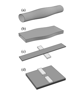
Figure 1: Schematic of various realisations of a near-perfect quantum wire. (a ) A cylindrical and (b) a rectangular wire with a bulge. (c) A gated straight wire. (d) Quantum point contact.

A general Hamiltonian for the two-electron problem has the form

$$H=-\frac{\hbar^{2}}{2m}\left[\frac{\partial^{2}}{\partial x_{1}^{2}}+\frac{\partial^{2}}{\partial x_{2}^{2}}\right]+v(x_{1})+v(x_{2})+V(x_{1},x_{2}).$$ (1)

In this equation we assume sufficiently high confinement that only the lowest non-degenerate transverse mode (channel) is occupied and the two electrons move in the effective one-electron potential, $v(x)$, with effective-mass $m$. This is not a serious restriction and corrections due to occupation of higher transverse mode, either due to thermal excitation or inter-channel coupling, may readily be accounted for perturbatively. The analysis and results may be extended to cases where there is degeneracy but we will not consider them here since our main aim is to emphasise the generic effects in the simplest and most direct way. The one-electron potential accounts for potential fluctuations due to disorder or smooth potential changes due to external gates, for example in a quantum-dot structure where they would model barriers. We shall be particularly interested in near-perfect wires for which $v(x)$ represents a shallow potential well (open quantum dot) that will bind a single electron, but not two electrons. The Coulomb interaction between the two electrons, $V(x_{1},x_{2})$, may be derived explicitly by starting with the usual 3D form and integrating over the lowest occupied transverse mode. The resulting expression, to a very good approximation, takes the simplified form $V(x_{1},x_{2})=e^{2}/\epsilon r$, where $r=\sqrt{(x_{1}-x_{2})^{2}+\lambda^{2}}$ is the effective separation and $\lambda$ is a parameter that characterised the transverse confinement, e.g., $\lambda\sim d$ for a circular wire of diameter $d$ [14].

We now consider the two-electron scattering problem in which a single electron is first introduced into the quantum wire and becomes bound in the quantum-dot region. The confining potential for this electron is determined completely by the one-electron potential $v(x)$. To be specific, we shall mainly consider a quantum wire with material parameters appropriate to GaAs, i.e. $m=0.067m_{0}$ and $\epsilon=12.5$, and a potential profile with $v(x)=-v_{0}\cos^{2}\pi x/L$ for $-L/2<x<L/2$ and zero otherwise. One motivation for studying this problem is the rapidly emerging field of quantum information processing in which a major goal is the generation of entanglement the controlled exchange of quantum information between propagating and static qubits. Purely electron systems have potential as entanglers due to strong Coulomb interactions and although charge-qubit systems suffer from short coherence times, spins in semiconductor quantum wires and dots are sufficiently long-lived for spin-qubits to be promising candidate for realising quantum gates involving both static and propagating spins [21, 22, 23, 24, 25]. Electron entanglers have been proposed using a double-dot, exploiting the singlet ground state [26]; the exchange interaction between conduction electrons in a single dot [27, 28]; and the exchange interaction between electron spins in parallel surface acoustic wave channels [29]. Measurement of entanglement between propagating electron pairs has also been proposed using an electron beamsplitter [30]. A further motivation for solving the two-electron scattering problem is that the solutions may be used directly in expressions for conductance and other transport quantities, which we consider in the next section.

Before presenting detailed numerical results, consider the expected general features when a spin-up propagating electron interacts with a bound electron in some arbitrary state on the Bloch sphere, i.e. $\cos(\vartheta/2)\left|\downarrow\right>+e^{i\phi}\sin(\vartheta/2)\left|\uparrow\right>$. In practise this situation may be realised, at least in principle, by a system in which single spin-polarised electrons are introduced into the wire through a turnstile injector. This first electron is then allowed to relax into the ground-state of the quantum dot region and its spin is subsequently manipulated on the Bloch sphere using microwave pulses. The second spin-up electron then scatters from this bound electron. It is important to realise that this two electron state before scattering is unentangled and is not an eigenstate of the Hamiltoninan Eq. (1). It may be written,

$$\Psi_{\mathrm{in}}=\cos(\theta/2)\Psi_{\uparrow\downarrow}+e^{i\phi}\sin(\theta/2)\Psi_{\uparrow\uparrow},$$ (2)

where

$$\Psi_{\sigma\sigma^{\prime}}=e^{ikx_{1}}\psi_{0}(x_{2})\chi_{\sigma}(\sigma_{1})\chi_{\sigma^{\prime}}(\sigma_{2})-e^{ikx_{2}}\psi_{0}(x_{1})\chi_{\sigma}(\sigma_{2})\chi_{\sigma^{\prime}}(\sigma_{1}).$$ (3)

Here $\psi_{0}$ is the bound-state wavefunction for the quantum-dot region and $\chi_{\sigma}(\sigma_{1,2})$ is a spin-1/2 spinor for an electron with spin $\sigma_{1,2}$.

During the scattering process the two electrons interact resulting in reflection or transmission. The scattered component resulting from $\Psi_{\uparrow\downarrow}$ in Eq. (2) can be either spin-flip or non-spin-flip scattered with corresponding amplitudes $r_{\mathrm{sf}}$, $r_{\mathrm{nsf}}$, $t_{\mathrm{sf}}$ and $t_{\mathrm{nsf}}$ for reflection and transmission. Spin-flip scattering is due to an exchange interaction between bound and propagating electrons. This is not a direct interaction between spins of the electrons since the Hamiltonian Eq. (1) does not contain any explicit spin-spin terms. It arises purely because of the antisymmetry of the two-electron wavefunction and their mutual Coulomb repulsion. The transmitted component is

$$\Psi_{\mathrm{trans}}=\cos(\theta/2)[t_{\mathrm{nsf}}\Psi_{\uparrow\downarrow}+t_{\mathrm{sf}}\Psi_{\downarrow\uparrow}]+e^{i\phi}\sin(\theta/2)\Psi_{\uparrow\uparrow}$$ (4)

with a similar expression for reflection.

After scattering, the propagating electron will be reflected or transmitted and, asymptotically, will have the same magnitude of momentum, $k$, leaving the bound electron again in its ground state, provided the kinetic energy of the incoming electron is chosen to be less than the binding energy of the bound electron. It is convenient and instructive to express these amplitudes in terms of eigenstates of the Hamiltonian, which have definite total spin since $[H,S^{2}]=[H,S^{z}]=0$. For 2 electrons the eigenstates are either singlets or triplets with $\Psi_{00}=(\Psi_{\uparrow\downarrow}-\Psi_{\downarrow\uparrow})/\sqrt{2}$, $\Psi_{10}=(\Psi_{\uparrow\downarrow}+\Psi_{\downarrow\uparrow})/\sqrt{2}$, $\Psi_{11}=\Psi_{\uparrow\uparrow}$, and $\Psi_{1,-1}=\Psi_{\downarrow\downarrow}$. Substituting these expressions into Eqs. (2), (3) and (4) we see directly that,

$$t_{\mathrm{nsf}}=\frac{t_{1}+t_{0}}{2}\>\textrm{and}\>t_{\mathrm{sf}}=\frac{t_{1}-t_{0}}{2},$$ (5)

where $t_{0}$ and $t_{1}$ are the singlet and triplet transmission amplitudes, respectively. Both the reflected and transmitted waves show spin entanglement after scattering provided $\cos(\vartheta/2)$ and the amplitudes for spin-flip and non-spin-flip scattering, $r_{\mathrm{sf}},\,r_{\mathrm{nsf}},\,t_{\mathrm{sf}}$ and $t_{\mathrm{nsf}}$ are non-zero. Furthermore, fully entangled states occur when $\vartheta=0$ and $|r_{\mathrm{sf}}|=|r_{\mathrm{nsf}}|$ or $|t_{\mathrm{sf}}|=|t_{\mathrm{nsf}}|$. It follows directly from this that one way of achieving maximum entanglement would be via either a singlet or triplet resonance. More precisely, if either $|t_{0}|=1$, $|t_{1}|=0$, or $|t_{1}|=1$, $|t_{0}|=0$ then the transmitted state will correspond to full entanglement between the transmitted electron and the electron remaining in the quantum dot. This has a simple physical interpretation. The initial (unentangled) state is the sum of a singlet state and an $S^{z}=0$ triplet state and only one of these components is transmitted or ’filtered’. Since either a singlet or a triplet state is fully entangled, such filtering via resonance produces a fully entangled static-flying spin-qubit pair with probability 1/2. Furthermore, the reflected state would also be fully entangled but with the complementary component. In this way the initial unentangled state is divided into its fully entangled singlet and triplet components, separated by transmission and reflection.

In practise it is not immediately obvious that such resonances will occur in quantum wires and in any case, the transmission of the complementary component is not expected to be precisely zero so the question arises as to whether perfect entanglement can still be achieved. In fact, the two-electron system in which there is a shallow quantum well will always have at least a singlet resonance.

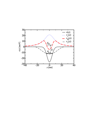
Figure 2: A shallow potential well $v(x)$ (full line) and the corresponding Hartree potential seen by a second electron of opposite spin (dashed line). The single resonant bound state, $\epsilon_{b}$, and quasi-bound singlet state, $\epsilon_{0}$, within the double barrier structure are also indicated. The dotted line is the Coulomb repulsion energy due to bound electron and the dashed-dotted line represents shallow potential well $v_{1}(x)$ corresponding for the results from Fig. 3(b).

This two-electron system has at least a singlet resonance ($|t_{0}|=1)$ at some energy for which the triplet state is off resonance $(|t_{1}|\ll 1)$, as may be seen from explicit solutions of the scattering problem. We may choose the shallow effective potential, $v(x)$, such that there is only a single one-electron bound state. For example, with a well depth of $26$ meV and a width of $\sim 20$ nm (Fig. 2) there is a single bound state at energy $\epsilon_{b}=-12$ meV. The bound electron has a long-range Coulomb interaction with the propagating electron and, when combined with the well potential, gives rise to a double barrier structure which has a singlet resonance energy at approximately $\epsilon_{0}\sim\epsilon_{b}+U$, where $\epsilon_{b}$ is the energy of the lowest bound state and $U=15$ meV is the Coulomb matrix element for two electrons of opposite spin occupying this state. This is also shown in Fig. 2 where we have plotted the Hartree potential due to the bound electron, $v_{\mathrm{H}}(x)$, i.e. the self-consistent potential seen by the propagating electron in the ’frozen’ potential due to the bound electron of opposite spin. For wider wells a second bound state is allowed and this will give rise to a triplet resonance (and a further singlet resonance) at higher energy. The singlet-triplet separation may be controlled by changing the width and depth of the well whilst maintaining the condition that only one electron be bound. With increasing well-width (and decreasing well-depth) the singlet-triplet separation reduces and eventually the resonances overlap.

At the lowest (singlet) resonance, $|t_{\mathrm{sf}}|\approx|t_{\mathrm{nsf}}|\approx\frac{1}{2}$ and the state is close to being fully entangled when spins are initially antiparallel ($\cos(\vartheta/2)=1)$. Similarly, in reflection, $|r_{0}|\approx 0$, $|r_{1}|\approx 1$ and $|r_{\mathrm{sf}}|\approx|r_{\mathrm{nsf}}|\approx\frac{1}{2}$, which is also close to being fully entangled. The precise condition for full entanglement in transmission, when the triplet component is not precisely zero is $\vartheta=0,$ $|t_{1}+t_{0}|=|t_{1}-t_{0}|$. This may be seen directly from the form of asymptotic outgoing states. When the scattered components are not fully entangled, we need a quantitative measure of entanglement which reduces to unity for fully entangled states and zero for unentangled states. Such a measure is the concurrence which, for the pure states considered here, takes the form Ref. [31]

$$C=2|\langle\Psi|\Psi_{\downarrow\downarrow}\rangle\langle\Psi|\Psi_{\uparrow\uparrow}\rangle-\langle\Psi|\Psi_{\uparrow\downarrow}\rangle\langle\Psi|\Psi_{\downarrow\uparrow}\rangle|,$$ (6)

where $\Psi$ is the scattered component in either transmission or reflection. We can see immediately from this expression that $C=1$ for fully entangled states, such as a singlet or $S^{z}=0$ triplet state, and zero for an unentangled state, such as $\Psi=\Psi_{\uparrow\downarrow}$. Substituting Eq. (4) into Eq. (6), the concurrence becomes

$$C=\frac{2\cos^{2}(\vartheta/2)|t_{\mathrm{sf}}\,t_{\mathrm{nsf}}|}{\cos^{2}(\vartheta/2)\left[|t_{\mathrm{sf}}|^{2}+|t_{\mathrm{nsf}}|^{2}\right]+\sin^{2}(\vartheta/2)|t_{\mathrm{sf}}+t_{\mathrm{nsf}}|^{2}}.$$ (7)

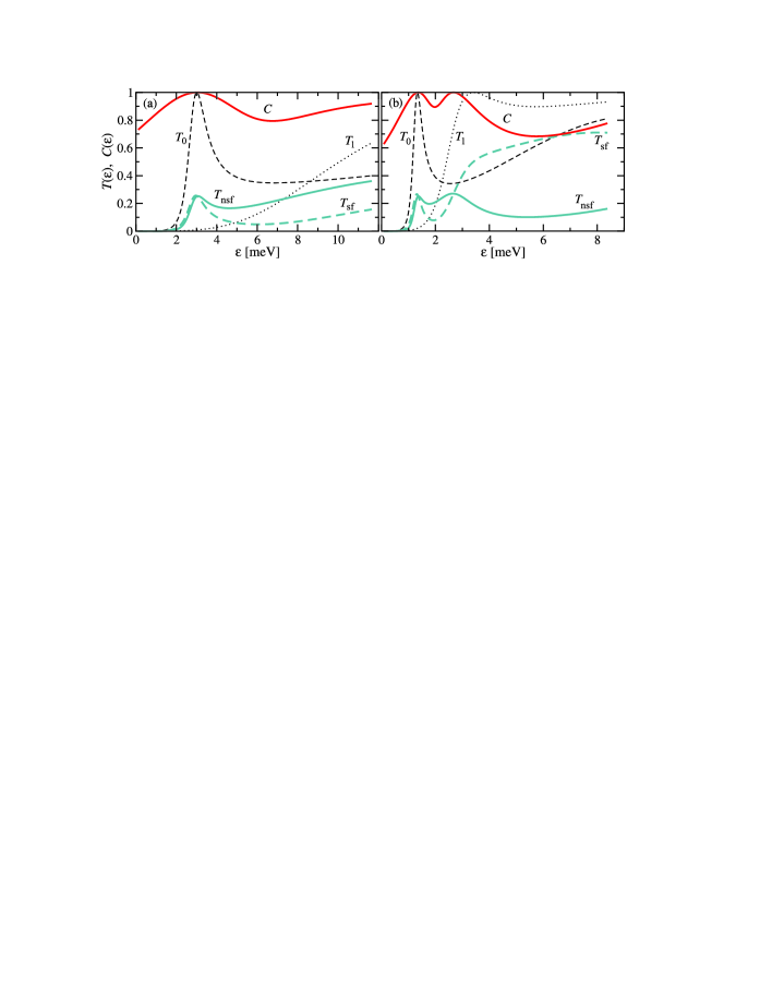
Figure 3: (a) Singlet and triplet transmission probabilities ($T_{S}=|t_{S}|^{2}$), spin-flip and non-spin-flip transmission probabilities and corresponding concurrence $C$ for confining potential $v(x)$ from Fig. 2. (b) Results for a shallower and longer potential, corresponding to $v_{1}(x)$ from Fig. 2.

Further illustration of this behaviour is seen by solving the scattering problem explicitly for specific cases. Numerical solutions for symmetrised (singlet) or antisymmetrised (triplet) orbital states yield directly the complex amplitudes $t_{0},\,r_{0},\,t_{1},\,r_{1}$ from which the amplitudes for spin-flip and non-spin-flip scattering may be calculated using Eq. (5).

In Fig. 3(a) we plot the singlet and triplet transmission and reflection probabilities, showing a single maximum of unity for the transmission. We also plot concurrence, which reaches a maximum value very close to the corresponding singlet resonance, occurring when the spin-flip probabilities are equal and approximately $\frac{1}{4}$ in both transmission and reflection. In Fig. 3(b) we show results for a shallow potential well of depth $12$ meV and width $\sim 40$ nm. With these parameters there are two single-electron bound states at energies $-8$ meV and $-10$ meV. This gives both a singlet and a triplet resonance, the latter corresponding to one electron in the lowest bound state and the other in the higher bound state which becomes a resonance obeying Hund’s rule under Coulomb repulsion, with a further singlet resonance outside the energy window for elastic scattering. We see that there are two unitary peaks of concurrence in transmission with the second close to, but clearly discernible from, the peak of the rather broad triplet resonance.

Thus we have shown that spin-entanglement and exchange of quantum information occurs via the Coulomb interaction when a propagating electron interacts Coulombically with a single bound electron in a shallow potential well in a one-dimensional semiconducting quantum wire. The degree of entanglement may be controlled by kinetic energy of the incoming electron and the shape of the effective potential well and unitary concurrence occurs near a singlet or triplet resonance. Potential realisations of such a system are semiconductor quantum wires and carbon nanotubes.

We conclude this section by describing the differences between the case of a near perfect quantum wire, or open quantum dot, described above and a ’real’ quantum dot defined by barriers. The presence of barriers, which in practise may be produced by further gates in 2DES systems, give the well-known single-electron tunneling resonances when the kinetic energy of the incoming electron is resonant with a quasi-bound state in the quantum dot. The first resonance occurs when there is no energy cost for a single-electron for hop onto or off the dot and the charge on the dot fluctuates between 0 and 1, with no real bound state. There is no such single-electron regime in the quantum wire case for which there is a real bound state that will bind one electron. In the case of the quantum dot, a second single-electron tunnel-ling regime occurs when the depth of the potential well is increased so that one electron is now in a real bound state and a second electron of opposite spin may resonantly tunnel on and off the dot at energy $U$ higher than the bound state, where $U$ is the intra-dot Coulomb matrix element. This also occurs in the quantum wire case but here the barriers arise solely from the Coulomb repulsion between the two electrons. One consequence of this is that at higher energies than the resonance, after an initial dip the transmission tends smoothly to unity, as shown in Fig. 3, whereas in the dot case the conductance remains low away from resonance. However, in other respects the two systems behave in a similar way, giving full entanglement near a two-electron resonance.

3 Many-electron problem and transport anomalies

Close to the conduction edge in a near-perfect quantum wire we again conjecture that a single electron becomes bound in a shallow potential well, or open quantum dot, along the wire. This then gives rise to spin-dependent scattering of conduction electrons and since we are close to the threshold for conduction it is reasonable to assume that the system will be dominated by sequential pairwise scattering. At each scattering event, total $S,S_{z}$ are conserved since, by assumption, there are no explicit spin-terms in the Hamiltonian. Hence, when the spins are parallel their direction cannot change in the scattering process. On the other hand, there will be both spin-flip or non-spin-flip scattering when the two electrons initially have opposite spin. This is a consequence of the effective exchange interaction between the spins, resulting from the Coulomb interaction and Pauli exclusion. As shown in the previous section, this is particularly pronounced when we are close to either a singlet or a triplet resonance for which a transmitted electron (with transmission probability  1/2) is fully entangled with the bound electron left behind, i.e. the scattering process acts as a spin filter of the initial state with equal probabilities of spin-flip and non-spin-flip transmission. More generally, if we sum over all incident electrons near the Fermi energy then, using the pairwise scattering solutions derived in the previous section, we may derive expression for transport quantities. We expect anomalies in these quantities when the Fermi energy is close to either a singlet or a triplet resonance. For the former, approximately $1/4$ of electrons are transmitted since half of them have spin parallel to the bound electron and of the remaining half, with spin antiparallel, approximately half are transmitted (singlet spin filter). This gives a total transmission of order $1/4$ when Fermi energy is close to the singlet resonance energy. On the other hand, close to a triplet resonance (at higher energy than the singlet resonance), of order $3/4$ of the electrons are transmitted. In what follows, we argue that these spin-dependent resonances are the main source of the transport anomalies observed in near perfect quantum wires.

3.1 Conductance anomalies

In the spirit of the Landauer-Büttiker approach [33], we may determine the current in a quantum wire or point contact from transmission probabilities. From equations (4) and (5), the total transmission probability for an incident spin-up electron interacting with a bound spin-down electron is

$$T_{\uparrow\downarrow}=|t_{\mathrm{sf}}|^{2}+|t_{\mathrm{nsf}}|^{2}={1\over 2}(|t_{0}|^{2}+|t_{1}|^{2}).$$ (8)

This is the same as the transmission probability for a propagating spin-down electron interacting with a bound spin-up electron, $T_{\downarrow\uparrow}$. When both propagating electrons have the same spin the transmission probability is that of a triplet component, i.e., $T_{\uparrow\uparrow}=T_{\downarrow\downarrow}=|t_{0}|^{2}$. Summing over all electrons in source and drain leads, with equal probabilities that the bound electron is initially spin-up or spin-down, gives directly the genealised Landauer-Büttiker formula [14],

$$I=\frac{2e}{h}\int(\frac{1}{4}T_{0}+\frac{3}{4}T_{1})(f_{L}-f_{R})d\epsilon,$$ (9)

where $T_{S}=T_{S}(\epsilon)$ are the energy dependent singlet or triplet transmission probabilities for $S=0$ and $S=1$, respectively. $f_{L,R}=\{1+\exp[(\epsilon-\mu_{L,R})/k_{B}T]\}^{-1}$ is the usual Fermi distribution function corresponding to left and right lead, respectively, with temperature $T$ and the Boltzmann constant $k_{B}$.

When the wire is connected to metallic source-drain contacts, electrons will flow into the wire region provided that the Fermi energy in the contacts is higher than the lowest allowed eigen-energy in the wire. As the Fermi energy is raised from below the conduction band edge in the wire (via a gate not considered explicitly), at least one electron will become bound in the shallow-well region of the wire. The number of bound electrons depends on both the Fermi energy and the relative depth and width of the well. As we have already stated, the parameters are chosen such that only one electron is bound. In Fig. 4 we show plots of the conductance $G=\mathrm{d}I/\mathrm{dV}$ where $V=-(\mu_{L}-\mu_{R})/e$ is the voltage difference between the leads, for two typical wires. Similar results are obtained for wires with thickness, $a$, up to $a\thicksim 50$ nm, beyond which the single-channel approximation becomes less reliable as electron correlations become increasingly important [34].

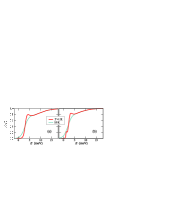
Figure 4: The conductance as calculated from Eq. (9) at $T=1$ K and $T=10$ K for two different wires with thickness $a=10$ nm: (a) $L=40$ nm and $v_{0}=19$ meV; (b) $L=50$ nm and $v_{0}=13$ meV.

The main feature of these results is that there are resonances in both singlet and triplet channels and these give rise to structures in the rising edge to the first conductance plateau for $G\sim\frac{1}{4}G_{0}$ (singlet) and $G\sim\frac{3}{4}G_{0}$ (triplet), with $G_{0}=2e^{2}/h$. The system is therefore in the regime where the incident electron sees a double barrier which will have some resonant energy for which there is perfect transmission. A more detailed analysis has to account for spin and this may be understood by gradually switching on the Coulomb interaction. For the present choice of parameters, and also a range of parameter sets which correspond to a very shallow well, there are two bound states for one electron. With no interaction both electrons may thus occupy one of 4 states (3 singlets and a triplet). If we now switch on a small Coulomb interaction then the lowest two-electron state will be a singlet, derived from both electrons in the lowest one-electron state. We may regard one electron as occupying the lowest bound-state level and the other electron of opposite spin also in this same orbital state but energy $U$ higher, where $U$ is the intra-‘atomic’ Coulomb matrix element, as in the Anderson impurity model. As the Coulomb interaction is increased, $U$ eventually exceeds the binding energy and this higher level becomes a virtual bound state giving rise to a resonance in transmission. An estimate of the energy of the virtual bound state is given by the Anderson Coulomb matrix element with both electrons in the one-electron orbital. For even weaker confinement in which the length $L$ of the quantum dot exceeds the effective Bohr radius of the electrons, the resonant bound states become strongly correlated with the electron density tending to peak at opposite ends of the dot-region in order to minimise their electrostatic repulsion energy. This situation could occur in carbon nanotubes, for example, where the Bohr radius is very small [20]. For such quantum dots there is a low-lying singlet-triplet pair isolated from higher-lying singlets and triplets. Thus we again have a single singlet resonance and a single triplet resonance that dominates the conductance near threshold.

In summary, within this simple formalism has been shown that quantum wires with weak longitudinal confinement can give rise to spin-dependent, Coulomb blockade resonances when a single electron is bound in the confined region, a universal effect in one-dimensional systems with very weak longitudinal confinement. The positions of the resulting features at $G\sim\frac{1}{4}G_{0}$ and $G\sim\frac{3}{4}G_{0}$ are a consequence of the singlet and triplet nature of the resonances.

3.2 Thermopower

The formalism applied above can be extended to include electrical and heat currents through a region between two leads with different temperatures and chemical potentials [35, 36]. With $T+\Delta T$, $\mu+eU$ for the left lead and $T$, $\mu$ for the right lead, we get the electric current $j_{e}$ and the heat current $j_{Q}$

$$I_{\mathrm{e}} = \frac{2e}{h}\int(\frac{1}{4}T_{0}+\frac{3}{4}T_{1})\Delta f(\epsilon){\mathrm{d}}\epsilon,$$ (10)

$$I_{\mathrm{Q}} = \frac{2}{h}\int(\epsilon-\mu)(\frac{1}{4}T_{0}+\frac{3}{4}T_{1})\Delta f(\epsilon){\mathrm{d}}\epsilon,$$ (11)

with

$$\Delta f(\epsilon)=f(\epsilon,\mu+eU,T+\Delta T)-f(\epsilon,\mu,T).$$ (12)

Figure 5: (a) Electrical conductance $G(\mu)$, (b) thermopower $S(\mu)$, and (c) thermal conductance $\kappa(\mu)$ for circular wire with parameters $a=10$ nm, $L=60$ nm, $v_{0}=12$ meV. Other parameters and the numerical method is as in Ref. [14] The dashed line in (c) represents Wiedemann-Franz law result for $T=4$ K. The traces for different $T$ are offset vertically for clarity.

The Seebeck thermopower coefficient $S$ was for various systems discussed in Refs. [36, 37]. It measures the voltage difference needed to neutralise the current due to the temperature difference between the leads. In the linear response regime the thermopower is in our model given by [38]

$$S(\mu)=\frac{U}{\Delta T}=-\frac{1}{eT}\frac{K_{1}(\mu)}{K_{0}(\mu)},$$ (13)

where

$$K_{n}(\mu)=-\int(\epsilon-\mu)^{n}(\frac{1}{4}T_{0}+\frac{3}{4}T_{1})\frac{\partial f(\epsilon,\mu,T)}{\partial\epsilon}{\mathrm{d}}\epsilon.$$ (14)

Eq. (13) is formally the same as the Mott-Jones formula for simple metals [39] and generalized for a system with stronger electron-phonon interactions in Refs. [40].

In Fig. 5(a) the conductance is shown for a wire with a bulge for different temperatures. The effect of temperature is accounted only through the temperature of the Fermi function in Eq. (12). Here the energy is measured from the threshold of the conductance. In this case both, singlet and triplet resonances contribute. In Fig. 5(b) the thermopower is presented for the same range of temperatures. In the thermopower curve the dominant structure at lower temperatures comes from the singlet resonance, though the triplet resonance is still clearly discernible. At higher temperatures the triplet structure is washed out first, in contrast to the conductance result, Fig. 5(a). The thermopower of one-dimensional wires has been measured [41, 42] and more recently, further anomalies related to ‘0.7 anomaly’ in conductance were reported [37]. The authors of Ref. [37] observe a dip in $S(\mu)$ at energies corresponding to the anomaly in $G(\mu)$. However, the logarithmic derivative with respect to the gate voltage of the measured $G$ exhibits a much deeper minimum than the dip in the measured $S(\mu)$, which remains well above zero even at the lowest temperatures. This clearly shows that a simple non-interacting formula is not valid in this low temperature regime. Apart from the small corrections to the logarithmic approximation to $S$, our results are in agreement with the findings of Ref. [37]. That is, the calculated thermopower is in good agreement with experiment except at low temperatures where we also predict a deep minimum. This discrepancy at low-temperatures may well be a many-body Kondo-like effect contained within our model [Eq. (18)] but not within the two-electron approximation we have used here. At very low temperatures, a Kondo-like resonance is expected [43], for which many-body effects would dominate with a breakdown of formula Eq. (13).

3.3 Thermal conductance

The linear thermal conductance is the heat current divided by the temperature difference between the leads when the chemical potentials are adjusted to give no electrical current. From Eqs. (10)-(14) we see that this is related to the transmission probabilities by,

$$\kappa(\mu)=\frac{2}{hT}\left(K_{2}(\mu)-\frac{K_{1}^{2}(\mu)}{K_{0}(\mu)}\right),$$ (15)

which for low temperatures simplifies to the Wiedemann-Franz law

$$\kappa(\mu)=\frac{\pi^{2}k_{\mathrm{B}}^{2}T}{3e^{2}}G(\mu).$$ (16)

In Fig. 5(c) $\kappa(\mu)$ is shown for $T$ from $0.2$ K to $3.8$ K. A comparison of Fig. 5(a) with Figs. 5(c) shows good agreement with the Wiedemann-Franz law at lower temperatures but there is increasing deviation at higher temperatures in the resonance region. For comparison, the dashed line in Fig. 5(c) shows the corresponding linear approximation result, i.e. the Wiedemann-Franz law. One of the most striking features of these plots is that $\kappa(\mu)$, calculated from Eq. (15), exhibits an anomaly at higher energies than the corresponding anomaly in conductance, a prediction which is open to experimental verification.

Within the framework of the Landauer-Büttiker approach thermal transport coefficients can be calculated for near-perfect semiconductor quantum wires, which extends the work on spin-dependent conduction anomalies. Thermopower and thermal conductance show anomalies, related ultimately to the Coulomb interaction between a localised electron and the remaining conduction electrons. We have shown that the lower-energy singlet anomalies in thermopower are more pronounced. These should be clearly observable in wires which show the corresponding conductance anomalies, such as the narrow ‘hard confined’ wires reported in Ref. [44], or in gated quantum wires under high source-drain bias where the singlet anomaly is clearly observed [45].

3.4 Shot noise and 0.7 anomaly

Recent high accuracy shot noise measurements enabled the extraction of the Fano factor in ballistic quantum wires [46]. The Fano factor $F$ is a convenient measure of the deviation from Poissonian shot noise. It is the ratio of the actual shot noise and the Poisson noise that would be measured in an independent-electron system [47]. This factor is, in our model [48],

$$F=\frac{\int[T_{0}(1-T_{0})+3T_{1}(1-T_{1})](f_{L}-f_{R})^{2}{\mathrm{d}}\epsilon}{\int(T_{0}+3T_{1})(f_{L}-f_{R})^{2}{\mathrm{d}}\epsilon}.$$ (17)

This expression and Eq. (9), are based on the results of a two-electron scattering between a single bound electron and a propagating conduction electron with a summation over all conduction electrons near the Fermi energy. This approximation is only valid at temperatures above the Kondo scale in this system [49], as discussed in Ref. [34]. Eq. (17) directly reflects the fact that singlet and triplet modes do not mix in this pairwise interaction approximation, resulting in contributions to the noise that add incoherently with the probability ratio 1:3 for singlet and triplet scattering.

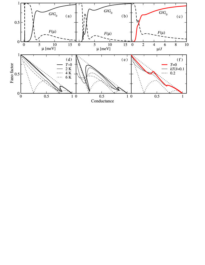
Figure 6: Results for a cylindrical quantum wires with a symmetric bulge for all parameters as in Fig. 3(b) and Fig. 3(c) of Ref. [14]. In panels (a) and (b) the conductance (full lines) and the Fano factor are presented. Panels (d) and (e): Fano factor as a function of $G$ (full line) and unitarity limits (dotted line). The energy dependence of the Fano factor and conductance for a left-right asymmetric confining potential (in resonance $T_{S}<1$), (c), and Fano factor as a function of conductance, (f). Energy and temperature scale is here in the units of single-triplet energy difference $J$.

The conductance $G(\mu)$ and Fano factor $F(\mu)$ are plotted vs $\mu$ in Fig. 6(a) and Fig. 6(b), with Fig. 6(d) and Fig. 6(e) showing the Fano factor $F$ vs $G$ for various temperatures and in the linear response regime, $\mu=\mu_{L}\sim\mu_{R}$. The dotted lines show zero temperature boundaries for the allowed values of $F$, under the assumption of validity of Eq. (17) in the limit $T\to 0$ and the unitarity condition for the transmission probabilities, $0\leq T_{S}\leq 1$. Eq. (17) is not strictly valid in the limit $T\to 0$ due to many-electron effects which start becoming important at low temperatures. Thus this zero-temperature limit should be regarded as a limiting behavior that would occur in the absence of such many-body effects. The Fano factor exhibits two distinctive features. Firstly, there is a structure for $G/G_{0}<0.5$ corresponding to the sharp $0.25$ singlet conductance anomaly. The second distinctive feature is in the region $0.5<G/G_{0}<1$ and corresponds to the dip in singlet channel just above the singlet resonance and also partially to the triplet channel resonance. In our previous work we assumed a symmetric confining potential fluctuation, giving perfect transmission probabilities at resonance energies. However, in real systems left-right symmetry will not be perfect, especially if the fluctuation is of random origin, and also under finite source-drain bias. In these cases $T_{S}<1$ even on resonance. Such an example is presented in Figs. 6(c, f). In this case the structure of $F(G)$ is less pronounced, consisting of kinks at $G/G_{0}\lesssim 0.5$ and $G/G_{0}\lesssim 0.75$. This behavior is a consequence of the absence of a pronounced triplet resonance and a dip in the singlet channel as mentioned above. Such a situation is typical for very weak confining potential fluctuations, where the triplet resonance is far in the continuum. The structure at $G/G_{0}\lesssim 0.5$ has the same origin as the ”0.25 structure” in conductance, a direct consequence of a sharp singlet resonance.

4 Many-body effects

Although the generic model we have used [Eq. (1)] is quite simplistic, it probably captures most of the essential physics. The many-electron generalisation of Eq. (1) may be obtained directly by expressing the Hamiltonian in second-quantised form using the solutions of the one electron problem, including both bound states in the well and unbound states in the wire. The resulting Anderson-like Hamiltonian [50] for the case of shallow well only, i.e. not quantum-dot barriers, takes the form [16, 34],

$$H = \sum_{k}\epsilon_{k}n_{k}+\epsilon_{d}n_{d}+\sum_{k\sigma}(V_{k}n_{d\bar{\sigma}}c_{k\sigma}^{\dagger}d_{\sigma}+\mathrm{h.c.})+$$ (18)

$$+ Un_{d\uparrow}n_{d\downarrow}+\sum_{kk^{\prime}\sigma}M_{kk^{\prime}}n_{d}c_{k\sigma}^{\dagger}c_{k^{\prime}\sigma}+\sum_{kk^{\prime}}J_{kk^{\prime}}{\bf S}_{\bf d}\cdot{\bf s}_{\bf kk^{\prime}}.$$

Here $U$ is the Hubbard repulsion, $V_{k}$ is the assisted hopping term, $M_{kk^{\prime}}$ corresponds to scattering of electrons and the direct exchange coupling is $J_{kk^{\prime}}$. Spin operators in Eq. (18) are defined as ${\bf S}_{\bf d}=\frac{1}{2}\sum_{\sigma\sigma^{\prime}}d_{\sigma}^{\dagger}{\hbox{\boldmath$\sigma$}}_{\sigma\sigma^{\prime}}d_{\sigma^{\prime}}$ and ${\bf s}_{\bf kk^{\prime}}=\frac{1}{2}\sum_{\sigma\sigma^{\prime}}c_{k\sigma}^{\dagger}{\hbox{\boldmath$\sigma$}}_{\sigma\sigma^{\prime}}c_{k^{\prime}\sigma^{\prime}}$, where the components of $\sigma$ are the usual Pauli matrices. A similar model has been proposed in Ref. [49]. Although the Hamiltonian, Eq. (18), is similar to the usual Anderson Hamiltonian [50], we stress the important difference that the $kd$-hybridization term above arises solely from the Coulomb interaction, whereas in the usual Anderson case it comes primarily from one-electron interactions. These have been completely eliminated above by solving the one-electron problem exactly. The resulting hybridization term contains the factor $n_{d\bar{\sigma}}$, and hence disappears when the localized orbital is unoccupied. This reflects the fact that an effective double-barrier structure and resonant bound state occurs via Coulomb repulsion only because of the presence of a localized electron. The above Hamiltonian is difficult to solve at low-energy/temperature, being in the class of many-body Kondo-like problems. However, as with the Kondo problem, we expect pairwise scattering solutions to capture the essential physics above the effective energy/temperature where condensation phenomena becomes important. It is this higher temperature scale that we have considered in this paper and the results presented are entirely equivalent to scattering solutions of the above Anderson-like model in the pairwise scattering approximation. We must await further research to fully elucidate low-temperature phenomena where it seems likely that the Kondo effect, that is clearly observed in conduction through quantum-dots, will be generalised to account for the suppression of conductance anomalies in the low-temperature regime. [51, 49]

5 Summary and conclusions

In this paper we have mainly focused on a generic model of a near-perfect quantum wire which contains a shallow quantum well which behaves like an open quantum dot that captures a single electron. We have not investigated in detail the actual causes of such a weak effective potential wells but point out that they may well be due to quite different sources in different experiments, e.g. thickness fluctuations, remote impurities or gates, electronic polarisation, or some other more subtle electron interaction effect. The main point is that because the effective potential well is shallow, it will bind one and only one electron and the subsequent spin-dependent scattering of a conduction electron from this bound electron can be used to induce entanglement between them. This is a consequence of resonant bound states arising from the Coulomb interaction. When this is combined with Pauli exclusion it gives rise to singlet and triplet resonances and the generation of entanglement may be interpreted as a filtering process in which either the singlet or triplet component of the initial unentangled state is reflected with complementary component being being transmitted. This same process is also responsible for transport anomalies when many conduction electrons (near the Fermi energy) scatter from a single bound electron. This is again a filtering effect in which  1/4 of incident electrons are transmitted when the Fermi energy is close the singlet resonance energy and  3/4 are transmitted close to the triplet resonance energy. The universal anomalies in conductance and thermopower are a direct consequence of this and occur for a wide range of circumstances in almost perfect quantum wires. This universal behaviour also occurs in quantum dots with ’real’ barriers which will also exhibit singlet/triplet spin-filtering and associated entanglement generation. However, for these cases the resonances will be much sharper reflecting the well-known Coulomb-blockade effect. If we imagine gradually increasing the quantum-dot barriers from zero then the anomalies in conductance will evolve into single-electron-tunneling resonances in the coherent transport regime, thus providing a unified picture of spin-dependent transport in quantum wire and quantum-dot structures.

References

References

- [1] J.R. Oppenheimer, Phys. Rev. 32, 361 (1928).
- [2] N.F. Mott, Proc. Roy. Soc. A 126, 259 (1930).
- [3] B.J. van Wees, H. van Houten, C.W.J. Beenakker, J.G. Williamson, L.P. Kouwenhoven, D. van der Marel, and C.T. Foxon, Phys. Rev. Lett. 60, 848 (1988).
- [4] D.A. Wharam, T.J. Thornton, R. Newbury, M. Pepper, H. Ahmed, J.E.F. Frost, D.G. Hasko, D.C. Peacock, D.A. Ritchie, and G.A.C. Jones, J. Phys. C 21, L209 (1988).
- [5] F.H.L. Koppens, C. Buizert, K.J. Tielrooij, I.T. Vink, K.C. Nowack, T. Meunier, L.P. Kouwenhoven, and L.M.K. Vandersypen, Nature 442, 766 (2006).
- [6] J.R. Petta, A.C. Johnson, J.M. Taylor, A. Yacoby, M.D. Lukin, C.M. Marcus, M.P. Hanson, and A.C. Gossard, Physica E 34, 42 (2006).
- [7] M. Kataoka, R.J. Schneble, A.L. Thorn, C.H.W. Barnes, C.J.B. Ford, D. Anderson, G.A.C. Jones, I. Farrer, D.A. Ritchie, and M. Pepper, Phys. Rev. Lett., 98 046801 (2007).
- [8] A. Yacoby, H.L. Stormer, Ned S. Wingreen, L.N. Pfeiffer, K.W. Baldwin, and K.W. West, Phys. Rev. Lett. 77, 4612 (1996).
- [9] A. Kristensen, P.E. Lindelof, J. Bo Jensen, M. Zaffalon, J. Hollingbery, S.W. Pedersen, J. Nygård, H. Bruus, S.M. Reimann, C.B. Sørensen, M. Michel, and A. Forchel, Physica B 249-251, 180 (1998).
- [10] S. De Franceschi, J.A. van Dam, E.P.A.M. Bakkers, L.-F. Feiner, L. Gurevich, and L.P. Kouwenhoven Apl. Phys. Lett. 83, 344 (2003).
- [11] T.S. Jespersen, M. Aagesen, C. Sørensen, P.E. Lindelof, and J. Nygård, Phys. Rev. B 74 233304 (2006).
- [12] H.I. Jørgensen, K. Grove-Rasmussen, J.R. Hauptmann, and P.E. Lindelof, Appl. Phys. Lett. 89 232113 (2006).
- [13] S.C. Benjamin, A. Ardavan, G.A.D. Briggs, D.A. Britz, D. Gunlycke, J.H. Jefferson, M.A.G. Jones, D.F. Leigh, B.W. Lovett, A.N. Khlobystov, S. Lyon, J.J.L. Morton, K. Porfyrakis, M.R. Sambrook, and A.M. Tyryshkin, J. Phys: Condens. Matter 18 S867 (2006).
- [14] T. Rejec, A. Ramšak, and J.H. Jefferson, Phys. Rev. B 62, 12985 (2000); J. phys., Condens. Matter 12, L233 (2000).
- [15] J.H. Jefferson, A. Ramšak, and T. Rejec, Phys. Low-dimens. Struct. 11-2 73 (2001).
- [16] T. Rejec, A. Ramšak, and J.H. Jefferson, in Kondo Effect and Dephasing in Low-Dimensional Metallic Systems, edited by V. Chandrasekhar, C. Van Haesendonck, and A. Zawadowski, NATO ARW, Ser. II, Vol. 50 (Kluwer, Dordrecht, 2001).
- [17] T. Rejec and Y. Meir, Nature 442 900 (2006).
- [18] O.P. Sushkov, Phys. Rev. B 67, 195318 (2003).
- [19] Y. Yoon, L. Mourokh, T. Morimoto, N. Aoki, Y. Ochiai, J. L. Reno, and J. P. Bird, Phys. Rev. Lett 99, 136805 (2007).
- [20] D. Gunlycke, J.H. Jefferson, T. Rejec, A. Ramšak, D.G. Pettifor, and G.A.D. Briggs, J. Phys.: Condens. Matter 18, S851 (2006).
- [21] D. Loss and D. P. DiVincenzo, Phys. Rev. A 57, 120 (1998).
- [22] J.M. Elzerman, R. Hanson, L.H. Willems van Beveren, B. Witkamp, L.M.K. Vandersypen, and L.P. Kouwenhoven, Nature 430, 431 (2004).
- [23] R. Hanson, B. Witkamp, L.M.K. Vandersypen, L.H. Willems van Beveren, J.M. Elzerman, and L.P. Kouwenhoven, Phys. Rev. Lett. 91, 196802 (2003).
- [24] R. Hanson, L.H. Willems van Beveren, I.T. Vink, J.M. Elzerman, W.J.M. Naber, F.H.L. Koppens, L.P. Kouwenhoven, and L.M.K. Vandersypen, Phys. Rev. Lett. 94, 196802 (2005).
- [25] J.R. Petta, A.C. Johnson, A. Yacoby, C.M. Marcus, M.P. Hanson, and A.C. Gossard, Phys. Rev. B. 72, 161301(R) (2005).
- [26] Xuedong Hu and S. Das Sarma, Phys. Rev. B 69, 115312 (2004).
- [27] A.T. Costa, Jr. and S. Bose, Phys. Rev. Lett. 87, 277901 (2001).
- [28] W.D. Oliver, F. Yamaguchi, and Y. Yamamoto, Phys. Rev. Lett. 88, 037901 (2002).
- [29] C.H.W. Barnes, J.M. Shilton, and A. M. Robinson, Phys. Rev. B 62, 8410 (2000).
- [30] G. Burkard and D. Loss, Phys. Rev. Lett. 91, 087903 (2004).
- [31] W.K. Wootters, Phys. Rev. Lett. 80, 2245 (1998).
- [32] J.H. Jefferson, A. Ramšak, and T. Rejec, Europhys. Lett. 75, 764 (2006).
- [33] R. Landauer, IBM J. Res. Dev. 1, 223 (1957); ibid. 32, 306 (1988); M. Büttiker, Phys. Rev. Lett. 57, 1761 (1986).
- [34] T. Rejec, A. Ramšak, and J.H. Jefferson, Phys. Rev. B 67, 075311 (2003).
- [35] U. Sivan and Y. Imry, Phys. Rev B 33, 551 (1986).
- [36] C.R. Proetto, Phys. Rev. B 44, 9096 (1991).
- [37] N.J. Appleyard, J.T. Nicholls, M. Pepper, W.R. Tribe, M.Y. Simmons, and D.A. Ritchie, Phys. Rev. B 62, R16275 (2000).
- [38] T. Rejec, A. Ramšak, and J.H. Jefferson, Phys. Rev. B 65, 235301 (2002).
- [39] N.F. Mott and H. Jones, The theory of the Properties of Metals and Alloys, 1st ed. (Clarendon, Oxford, 1936).
- [40] M. Jonson and G.D. Mahan, Phys. Rev. B, 21, 4223 (1980); ibid. 42, 9350 (1990).
- [41] N.J. Appleyard, J.T. Nicholls, M.Y. Simmons, W.R. Tribe, and M. Pepper, Phys. Rev. Lett. 81, 3491 (1998).
- [42] L.W. Molenkamp, H. van Houten, C.W.J. Beenakker, R. Eppenga, and C.T. Foxon, Phys. Rev. Lett. 65, 1052 (1990).
- [43] D. Boese and R. Fazio, Europhys. Lett. 56, 576 (2001).
- [44] D. Kaufman, Y. Berk, B. Dwir, A. Rudra, A. Palevski, and E. Kapon, Phys. Rev. B 59, R10433 (1999).
- [45] N.K. Patel, J.T. Nicholls, L. Martin-Moreno, M. Pepper, J. E. F. Frost, D. A. Ritchie, and G. A. C. Jones, Phys. Rev. B 44, 13549 (1991); K.J. Thomas, J.T. Nicholls, M.Y. Simmons, M. Pepper, D.R. Mace, D.A. Ritchie, Phil. Mag. B 77, 1213 (1998).
- [46] P. Roche, J. Ségala, D.C. Glattli, J.T. Nicholls, M. Pepper, A.C. Graham, K.J. Thomas, M.Y. Simmons, and D.A. Ritchie, Phys. Rev. Lett. 93, 116602 (2004).
- [47] Ya. M. Blanter and M. Büttiker, Phys. Rep. 336, 1 (2000).
- [48] A. Ramšak and J.H. Jefferson, Phys. Rev. B 71, 161311(R) (2005).
- [49] Y. Meir, K. Hirose, and N.S. Wingreen, Phys. Rev. Lett. 89, 196802 (2002).
- [50] P.W. Anderson, Phys. Rev 124, 41 (1961); G.D. Mahan, Many-Particle Physics (Plenum Press, New York, 1990).
- [51] S.M. Cronenwett, H.J. Lynch, D. Goldhaber-Gordon, L.P. Kouwenhoven, C.M. Marcus, K. Hirose, and N.S. Wingreen, and V. Umansky, Phys. Rev. Lett. 88, 226805 (2002).