Studying the X-ray hysteresis in GX 339-4: the disc and iron line over one decade

Abstract

We report on a comprehensive and consistent investigation into the X-ray emission from GX 339-4. All public observations in the 11 year RXTE archive were analysed. Three different types of model - single powerlaw, broken powerlaw and a disc + powerlaw - were fitted to investigate the evolution of the disc, along with a fixed gaussian component at $6.4{\rm\thinspace keV}$ to investigate any iron line in the spectrum. We show that the relative variation in flux and X-ray colour between the two best sampled outbursts are very similar. The decay of the disc temperature during the outburst is clearly seen in the soft state. The expected decay is $S_{\rm Disc}\propto T^{4}$; we measure $T^{4.75\pm 0.23}$. This implies that the inner disc radius is approximately constant in the soft state. We also show a significant anti-correlation between the iron line significant width and the X-ray flux in the soft state while in the hard state the $EW$ is independent of the flux. This results in hysteresis in the relation between X-ray flux and both line flux and $EW$. To compare the X-ray binary outburst to the behaviour seen in AGN, we construct a Disc Fraction Luminosity Diagram for GX 339-4, the first for an X-ray binary. The shape qualitatively matches that produced for AGN. Linking this with the radio emission from GX 339-4 the change in radio spectrum between the disc and power-law dominated states is clearly visible.

1 Introduction

The galactic X-ray binary GX 339-4 (=V821 Ara) was discovered by the OSO-7 satellite (Markert et al., 1973). The optical counterpart to the companion star of the compact object has not been detected. Therefore the system has been classed as a low-mass X-ray binary (XRB) from upper limits on the luminosity of the companion (Shahbaz et al., 2001). Hynes et al. (2004) using the non-detection and orbital parameters, conclude that the companion is probably a sub-giant, of spectral type G or later. Studies of the X-ray spectral and temporal characteristics conclude that it is a black hole X-ray binary (Zdziarski et al., 1998; Sunyaev & Revnivtsev, 2000); the characteristics of the Fourier power spectra are more similar to other black hole X-ray binaries, rather than those of neutron stars. For other studies of the X-ray emission from this source see e.g. Ueda et al. (1994); Zdziarski et al. (1998); Wilms et al. (1999); Kong et al. (2000); Wardziński et al. (2002); Zdziarski et al. (2004); Belloni et al. (2005).

Black hole X-ray binaries exhibit two main spectral states, the low-hard and the high-soft (e.g. van der Klis, 1995; McClintock & Remillard, 2006). In a variety of accretion models, the only parameter which determines the state of an X-ray binary is the mass accretion rate (e.g. Esin et al., 1997), however a number of phenomena indicate that other parameters are also important. The major one is the hysteresis of the state transition – the transition from low-hard to high-soft occurs at higher fluxes than the return to the low-hard from the high-soft state (e.g. Miyamoto et al., 1995). In addition, the luminosity of the source when the first state transition occurs varies from outburst to outburst (Belloni, 2006).

As described in detail in Fender et al. (2004), an average X-ray binary spends a large fraction of its time in the low-hard state. In this state radio emission indicates that the black hole is producing a steady radio-synchrotron emitting jet and the X-ray spectrum can be modelled by a hard powerlaw (photon index, $\Gamma\sim 1.5$). As the outburst progresses the luminosity of the binary increases and the X-ray spectrum softens. Eventually the jet disrupts and the X-ray spectrum is dominated by the soft disc emission. This is known the high-soft state. During the outburst, matter is accreted onto the black hole. The mass accretion rate reduces and disc is expected to cool, and therefore fade, as the outburst progresses. At the end of the outburst the spectrum hardens as the system returns to the low-hard state and the jet reforms.

RXTE was launched in December 1995 and has been observing GX 339-4 since June 1996. The archive of data built up over the intervening period allows an extensive investigation into the behaviour of GX 339-4 over a comparatively long baseline using the same instrument. The long term variability allows comparisons to be made between the four clear outbursts seen in the RXTE data. The large number of individual observations also allow detailed studies of single outbursts of GX 339-4.

In the hard state, GX 339-4 is a weak but steady radio source, with flux densities $\lesssim 15$ mJy at centimetre wavelengths and a flat spectrum (for a review see Fender et al., 1999). In the low-hard state there is a non-linear positive correlation between the radio flux and both the hard and soft X-ray fluxes (Corbel et al., 2000). This is likely to result from a coupling between the corona and the jet. Radio observations during the transition to the soft state have also seen ejection events which have been interpreted as large-scale relativistic radio jets (Fender et al., 1997; Gallo et al., 2004).

GX 339-4 regularly varies by 4-5 orders of magnitude in X-ray flux. This relatively high number of outbursts, from a very low quiescent state to a high state, makes GX 339-4 one of the most interesting galactic X-ray binary sources. Combining radio with X-ray observations of the source during an outburst led to the development of a physical explanation for the evolution of the source as the outburst progresses (Homan et al., 2001; Fender et al., 2004).

Black holes themselves are described by only two parameters, their mass and spin. The observational properties of the X-ray binary arise from the interplay of the parameters of the black hole (mass and spin) and those of the accretion flow (including the mass accretion rate through the disc). The black hole parameters are unlikely to change much on short timescales, and so it is the mass accretion rate and geometry of the accretion flow which is responsible for the large changes in the emission spectrum.

Recent developments have been made in creating unification schemes between X-ray binaries and Active Galactic Nuclei (AGN). The radio-X-ray flux relation for GX 339-4 was generalised to a large number of black hole X-ray binaries by Gallo et al. (2003). A scaling across a wide range of mass scales from X-ray binaries to AGN was subsequently presented by Merloni et al. (2003) and Falcke et al. (2004) and became known as the “fundamental plane”. Another plane using the timing properties of black holes has recently been constructed by McHardy et al. (2006) and Körding et al. (2007).

The observed variability timescales of AGN are many orders of magnitude longer than those in X-ray binaries. To study the evolution of an AGN outburst a population study is required. In order to be able to compare the outbursts of black hole binaries with AGN Körding et al. (2006) create a more general diagram to show the spectral states in AGN by comparing the disc flux and the power-law flux. We complement this by creating an equivalent diagram for this X-ray binary (see Section 7.

We present our data reduction scheme in Sections 2 and 3. Our investigations in to the iron line and the Disc are discussed in Sections 5 and 6, with the Radio correlations presented in Section 8.

2 Data Reduction

In order to fully investigate the existence and properties of the iron line and disc in GX 339-4, all observations in the RXTE archive were downloaded and analysed. This gave $2.59{\rm\thinspace Ms}$ of PCA exposure over an 11 year baseline for this study, containing the two well-sampled outbursts, as well as two other outbursts with fewer public RXTE observations.

All the data were reprocessed so all observations had the same version of the data reduction scripts applied. The HEXTE data were analysed so that the high energy spectral slope could be well constrained. This helps in fitting the lower energy spectrum. We use the data reduction tools from HEASOFT version 6.3.2. The data reduction and model fitting were automated so that each observation was treated in exactly the same way.

2.1 PCA Reduction

The PCA data were reduced according to the RXTE Cookbook, and only a quick summary is given here.

We used only data from PCU-2 as it is always switched on, and so can be used over the entire archive of data. It is also the best calibrated of the PCUs on RXTE. Background spectra were obtained using pcabackest from new filter files created using xtefilt, from which updated GTI files were also created. The spectra were extracted and the customary systematic error of 1 per cent was added to all spectra using grppha.

In order that the model fitting in xspec was reliable and relatively quick, we only fitted spectra which had more that 1000 background subtracted PCA counts. In total there were 913 spectra extracted from PCA data. Cutting those with fewer than 1000 counts from further analysis, removed 191 observations (the bottom 21 per cent), leaving 722. The excluded observations occur throughout the light curves of the outburst, with a concentration in the low flux periods. The low-luminosity observations with low counts fall into the “stalks” of the Hardness Intensity Diagrams. As our analysis concentrates on the disc parameters, excluding these observations is unlikely to bias our conclusions.

2.2 HEXTE Reduction

The HEXTE data were also reduced according to the RXTE Cookbook. Where possible, we used both Cluster A and Cluster B data. Background spectra were obtained using hxtback. Spectra were extracted using the routine appropriate to the data-type (Event or Archive). Dead-time was then calculated using hxtdead. All spectra for a given ObsID were then summed using sumpha, and the appropriate responses and ancillary files were added in as header key words using grppha. In total there were 701 spectra extracted from Cluster A data and 905 for Cluster B. In order to accurately determine the slope of the high energy power-law we require HEXTE data to be present when fitting a model. There have to be at least 2000 background subtracted counts in one of the HEXTE clusters, with the other having a positive number of counts. As our analysis concentrates on the properties of the disc and any emission line which might be present, we also require PCA data to be present in the spectra which are fitted.

3 Model Fitting

The spectra were fitted in xspec (v12.3.1ao). As our spectral analysis concentrates on the disc properties of GX 339-4, we wish to analyse the spectra to the lowest possible energies. The energy boundaries corresponding to channel numbers have changed during the lifetime of the RXTE mission. The calibration of channel numbers $\leq 6$ is uncertain, and we therefore ignore all PCA channels $\leq 6$ ($\sim 3{\rm\thinspace keV}$), which allows a consistent lower bound to the spectra, extending them to the lowest possible energies and maintaining calibration. All PCA data greater than $25{\rm\thinspace keV}$ were also ignored. The HEXTE data were fitted between $25$ and $250{\rm\thinspace keV}$. To investigate the presence or absence of an iron line and also to see whether any disc emission was present, three types of models were fitted: Powerlaw (power), Broken Powerlaw (bknpower) and Powerlaw + Disc (power+discbb). For each of these, a version including a Gaussian line fixed at $6.4{\rm\thinspace keV}$ was also fitted, giving a total of six models which were fitted to each spectrum. Galactic absorption was modelled using the wabs photoelectric absorption code, with a fixed $N_{\rm H}=0.4\times 10^{22}{\rm\thinspace cm^{-2}}$ (e.g. Miller et al., 2004b). Cabanac et al. (in prep.) discuss possible variations of the $N_{\rm H}$ during an outburst of GX 339-4. There is insufficient spectral coverage at lower energies to allow the $N_{\rm H}$ to remain free during the spectral fitting. To obtain fluxes outside of the RXTE observing band, for the disc for example, dummy responses were created within xspec.

To account for the galactic ridge emission, we add in the equivalent of a correction file to each spectrum. This has the greatest effect on the low flux observations. To model the galactic ridge emission, we used observations of GX 339-4 in Obs ID P91105 between MJD 53550 and 53650 (25 observations, 19.1 ks exposure). We assume that the emission in these observations is dominated by the galactic ridge, with almost no contribution from GX 339-4. We fit this data using an absorbed powerlaw with a gaussian emission line. The best-fit values ($\Gamma=2.127$, $\mathcal{N}_{\Gamma}=1.153\times 10^{-4}{\rm\thinspace keV^{-1}~{}cm^{2}~{}s^{-1}}$, line energy$=6.491{\rm\thinspace keV}$, $\sigma=1.729\times 10^{-3}{\rm\thinspace keV}$ and $\mathcal{N}_{\rm line}=1.07\times 10^{-6}{\rm\thinspace keV^{-1}~{}cm^{2}~{}s^{-1}}$), are added into each model fit as a fixed set of components to take account of the galactic ridge emission.

The high energy channels from HEXTE suffer from a high background leading to a low number of net counts in the low exposure time observations. This results in the high energy flux not being well determined. Using grppha, we investigated the effect of binning. The channels were binned so that there was a minimum number of counts within each bin. To have clearly defined fluxes at all HEXTE energies we found that the level of binning had to be very high, and the lower energies were then severely over-binned. However, the change in the value of the parameters, their uncertainties and the reduced $\chi^{2}$ changed very little, on the order of 5 per cent or less. We therefore do not perform any binning during the analysis of the data.

We encountered some difficulty in fitting discs reliably. The response of RXTE is only reliable down to $\sim 3{\rm\thinspace keV}$, whereas the disc we are trying to measure has a temperature of around $1{\rm\thinspace keV}$. We set the minimum disc temperature to $k_{\rm B}T=0.1{\rm\thinspace keV}$ in xspec to prevent discs from being fit at very low temperatures. It is likely that in cases where this occurred, the disc was being fit to take into account of any curvature in the powerlaw slope rather than to a true disc component. Before selecting the best fitting model we penalised disc models which had $k_{\rm B}T<0.4{\rm\thinspace keV}$. In doing this we note that we are likely to have excluded a few disc fits which are going to be reliable.

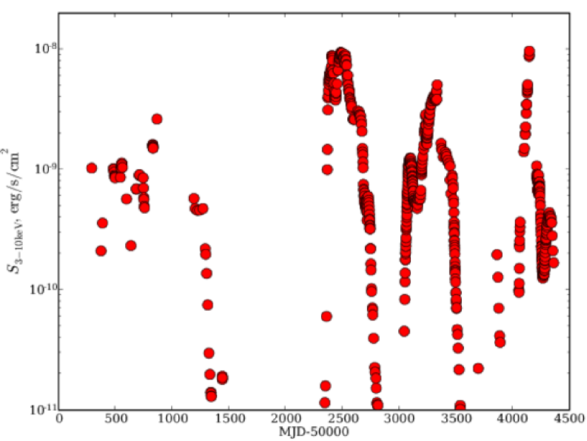
Figure 1: The RXTE-PCA lightcurve of GX 339-4 over 11 years. The flux is the absorbed flux between $3-10{\rm\thinspace keV}$.

We initially select the model with the lowest reduced $\chi^{2}$. However, if this best fitting model is a broken powerlaw or a disc+powerlaw model, we test whether using this more complex continuum model is a significant enough an improvement over a simple unbroken powerlaw, by performing an $F$-test. If the $F$-statistic probability $\mathcal{P}<0.001$ then we select the more complex continuum model. We investigated the number of discs deemed “significant” using different probability cut-offs. The number of discs was for all intents and purposes constant regardless of whether the probability cut-off was $0.05$ (234 disc detections) or $0.00001$ (214 disc detections). We can therefore be certain that almost all disc values used in the rest of the analysis are from significant discs, what ever cut-off we use

We note that we may be missing non-dominant disc components in, for example, the hard state. Even though we fit all observations with a powerlaw + disc model, the lack of sensitivity of the RXTE PCA below $\sim 3{\rm\thinspace keV}$ makes detecting non-dominant discs difficult. Therefore even if no significant disc is detected in our analysis, there may be discs present at a very low level in the hard and intermediate states – absence of evidence does not mean evidence of absence. See Section 4 for some higher signal-to-noise spectra and further discussion of disc components when GX 339-4 is not in the soft state.

To determine whether the gaussian component at $6.4{\rm\thinspace keV}$ is likely to be an accurate representation of a true iron line we followed the scheme outlined below. The line was deemed to be not well constrained when the width, $\sigma$, was larger than $1{\rm\thinspace keV}$. In these cases, although the best fitting model includes a line component, only the base continuum model was used for further analysis. Subsequently, an $F$-test was used to determine if the addition of the line was statistically significant ($\mathcal{P}<0.001$), and the appropriate model then chosen for further analysis.

We note that there have been recent doubts about the applicability and accuracy of using an $F$-test to determine the presence of a line and more complex continuum models. Protassov et al. (2002) state that the $F$-test does not adhere to the $F$ distribution, even asymptotically. As we are attempting to determine the presence of disc and line components, this is of importance to the work presented here. However, we note that the alternatives to an $F$-test are not easily implemented within the current fitting proceedure. Our solution is therefore as follows. A usual cut-off for a spectral feature to be significant is $\mathcal{P}<0.001$ (99.9 per cent confidence). We investigated the number of lines deemed “significant” using different $F$-probability cut-offs. There is a larger variation in the numbers of significant lines detected than in the equivalent investigation for the discs. Using a cut-off of $0.05$ there are 533 observations with lines deemed significant, but using $0.00001$ there are only 322. It is therefore not clear which $F$ probability to use as the cut-off for a significant line detection. Therefore we include the estimation of the line significance using the normalisation of the gaussian component.

This method uses the normalisation of the line component from xspec and its uncertainty. We use the uncertainty as an estimate of the normalisation sigma, and hence treat line components as significant if their normalisation differs from zero by at least three sigma. Both of these two statistical tests have to be satisfied for the line to be used in any further analysis. Using an $F$-test probability of $\mathcal{P}<0.001$ and significance of the line normalisation, results in 400 line detections. We do note that some may be erroneous “detections” but the majority will be true features in the spectrum, see also Section 4 and Fig. 5 for higher signal-to-noise spectra.

Any observation with a $3-10{\rm\thinspace keV}$ flux from the best fitting model of less than $1\times 10^{-11}{\rm\thinspace erg~{}s^{-1}}$ was also discarded from further analysis, as were ones where the flux was not well determined (the error on the $3-10{\rm\thinspace keV}$ flux was larger than the flux itself). This resulted in a final list of 628 observations, corresponding to $2.261{\rm\thinspace Ms}$, with well fitted spectra and high enough fluxes and counts. We extract a range of parameters and fluxes for different bands and model components which are presented and analysed further the following sections.

The full PCA lightcurve of GX 339-4 is shown in Fig. 1. There are four outbursts covered in this period: Outburst 1 from MJD-50000 = 0-1500, Outburst 2 from 2340-2800, Outburst 3 from 3040-3510 and Outburst 4 from 4000-. The MJD shown is for the midpoint of each individual observation. The best sampled outbursts are the middle two, and these are the ones on which some of the remaining analysis concentrates on as these have the most observations.

Following the analysis in e.g. Homan et al. (2001); Belloni (2004); Fender et al. (2004), we plot the X-ray observations in a Hardness-Intensity Diagram (HID) to show the state changes of GX 339-4 during its outbursts. We extract the $3-6$, $6-10$ and $3-10{\rm\thinspace keV}$ fluxes from the spectra. The X-ray colour was calculated from $S_{6-10{\rm\thinspace keV}}/S_{3-6{\rm\thinspace keV}}$ and plotted against $S_{3-10{\rm\thinspace keV}}$ in Fig. 2.

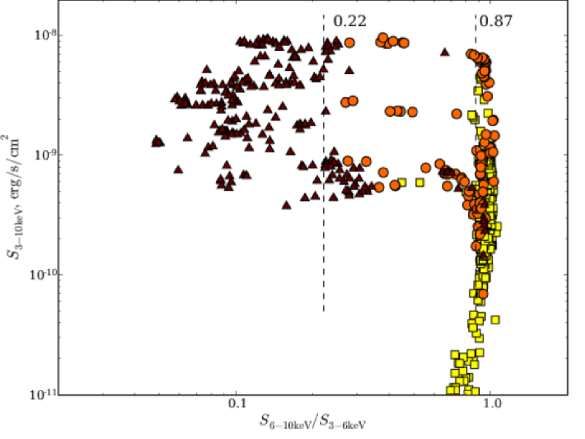
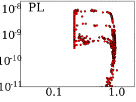
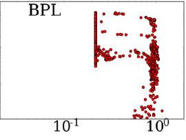
Figure 2: top: The hardness-intensity diagram from all the observations. Powerlaw models in squares, Broken Powerlaw models in circles, Powerlaw + Disc models in triangles – i.e. all triangular points require discs. X-ray colours of 0.225, 0.41 and 0.85 define the soft–soft-intermediate, soft-intermediate–hard intermediate and hard-intermediate–hard state transitions.bottom: The HIDs using a single continuum model only powerlaw (PL), broken powerlaw (BPL) and disc + powerlaw (DPL), left to right. The axes are the same scale as the main figure.

In Fig. 2 we show the X-ray colours of GX 339-4 where the state transitions between the high-soft and soft-intermediate states, as well as the hard-intermediate and low-hard states occur. The transitions have been determined by changes in the timing properties of the source as calculated in Belloni et al. (2006) using data corresponding to our Outburst 3 (see Section 4). Both transitions towards and away from the soft state occurred between observations such that a single X-ray colour could be used to delineate the state changes.

Belloni et al. (2005) study our Outburst 2 and the transitions from the hard state and into the soft state are very similar to those in Outburst 3 and so match those we use in this work. However, the transition between the hard- and soft-intermediate states occurs at a different X-ray colour. Also, there is no observation in soft-intermediate state on the return to the low-hard state in Outburst 2. The X-ray colour for the transition from the hard-intermediate to the soft-intermediate state in Outburst 3 is $S_{6-10{\rm\thinspace keV}}/S_{3-6{\rm\thinspace keV}}<0.37$.

There is no clear reason why the transition should occur at the same X-ray colour for any two outbursts. The X-ray colour is determined by the temperature and photon index, and also by the relative strength of the two components. The transitions towards the soft state are very different between the two outbursts, and so we should not expect the same X-ray colour to work for all three transitions. As a single X-ray colour could be determined for the transition between the two intermediate states in Outburst 3 we show this on the appropriate figures, but do not show an equivalent no figures for Outburst 2.

Initial investigations into the HID for the most recent outburst (Outburst 4) whose transition into the soft state occurred at a similar flux to Outburst 2, shows transitions between states calculated from X-ray timing, at similar X-ray colours to Outburst 2 (Del Santo et al., in prep.).

From now on we concentrate mainly on the soft and the hard states as these are the best sampled (e.g. Belloni, 2006). For the remainder of this work we define the soft state when the X-ray colour, $S_{6-10}/S_{3-6}<0.22$, and the hard state when $S_{6-10}/S_{3-6}>0.87$ unless stated otherwise (see Fig. 2), and the intermediate state is not split in any discussions.

We also show the HIDs obtained for GX 339-4 using each of the thee continuum models individually in Fig. 2. The basic shape of the HID is recovered in all three cases, with the most similar being the one for the disc + powerlaw. There is a clear “pile-up” of observations with an X-ray colour around 0.2, which is close to our adopted transition into the soft state. This is mainly the result of our restriction on the slope of the powerlaw to have $\Gamma<4.0$. This limit was set to aid the fitting of a disc. As the PCA is only sensitive down to $\sim 3{\rm\thinspace keV}$ the curvature of the disc component can be difficult to fit when the disc is not dominating the spectrum. Therefore a fit might result in an extremely steep powerlaw rather than a disc. Also, if there are insufficient HEXTE counts then the powerlaw slope cannot be well determined from the hard X-rays, which would allow an nonphysical steep powerlaw fit with the disc in the soft state. Powerlaws of $\Gamma>4.0$ are thought to be unphysical. The best fitting models just harder of this X-ray colour are ones with a disc component, and observations in the intermediate states which have broken powerlaw models as their best fit have well determined slopes not pegged at $4.0$. Therefore we do not believe that this restriction is influencing our results (see Section 4 for disc models in the intermediate state). There is little difference between the powerlaw and broken powerlaw models as the break usually occurs at around $10{\rm\thinspace keV}$ and so has little effect on the X-ray colour adopted here.

3.1 Comptonisation Models

We note that the powerlaw models we use here have limited physical meaning. We therefore performed a quick investigation into fitting the comptt model combined with a diskbb and gaussian line component to the data. Using this combination of models would result in a disc component being fitted whatever the state of the source and so would be a method for investigating the disc parameters outside of the soft state. Selecting the four hard state spectra with the greatest number of PCA counts resulted in a good fit with well defined values for the $\tau$ and $kT$ parameters, which were reasonably similar between different observations ($\sim 2.5$ and $\sim 25{\rm\thinspace keV}$ respectively).

However, turning to the soft state, again using four spectra with the largest number of PCA counts, we found that the lack of high energy counts from HEXTE meant that we could not determine both $\tau$ and $kT$ for every observation. Fixing $kT=50{\rm\thinspace keV}$, the average value from those observations where both parameters could be estimated, allowed a value of $\tau\sim 0.5$ to be estimated.

Using a single analysis scheme and script for all the observations is vital to remove any systematic differences between the analysis of different observations. As the values of both $\tau$ and $kT$ varied between the soft and hard states, and the fact that we were not able to determine independent values for both parameters in the observations of the soft state with the highest PCA counts, we did not investigate any further. The observations investigated with comptt had between 0.7 and 11 million PCA and 60 and 350 thousand HEXTE background subtracted counts, whereas our cut-off for the number of counts in an observation is 1000 PCA and 2000 HEXTE background subtracted counts. We do not believe that many well defined parameters will be extracted from fitting comptt models to these shorter, low counts observations.

3.2 Best Fitting Models

The description of the method used to select the best fitting model is outlined in Section 3. Fig. 2 shows which was the best fitting model through the HID. Models without the disc component are the best fitting for the majority of the hard and intermediate state observations. The soft state observations are exclusively best fit by models which include a disc component.

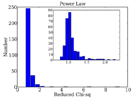
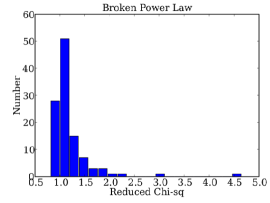
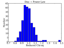
Figure 3: The distributions of the reduced $\chi^{2}$ for the three different continuum models selected as best fitting using the method presented in the text. The inset in the powerlaw model is an enlargement of the peak of the distribution.

However, some of the observations in the hard state have best fitting models which include a disc component. It is expected that the disc emission should be very low compared to the power-law emission when GX 339-4 is in the hard state. As a result it is surprising that for some hard state observations the best fit model includes a disc component. It is likely that, although these models have the lowest $\chi^{2}$ from the ones fitted, their disc parameters are not accurate. These disc fluxes are one to two orders of magnitude below those from observations in the soft state. The errors on the disc temperature from these fits are larger than those obtained from observations in the soft state. A combination of a broken power-law and the galactic absorption may have combined to emulate the emission from a disc sufficiently that a disc model is the best fitting.

Other X-ray missions (e.g. Swift, XMM-Newton) have a response at low energies such that, if a disc were present in the hard state, then they would be able to detect it in a suitable length observation. In GX 339-4  Cabanac et al. (in prep.) detect discs outside of the soft state, as do Miller et al. (2006). However, in the closer source XTE J1118+480 discs have been seen in the hard state Chaty et al. (2003); McClintock et al. (2001).

The distributions of the reduced $\chi^{2}$ for the three best fitting continuum models are shown in Fig. 3. The range in $\chi^{2}$ for the three continuum models is on the whole between $0.8\to 1.5$ with some outliers. Most outliers are in the simple power-law model fits as this is the default model, but they are few in number.

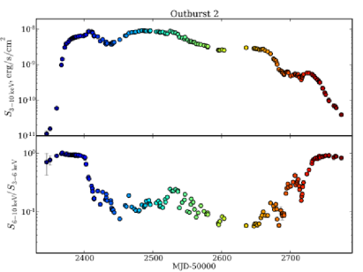
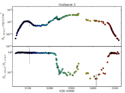
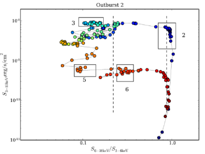
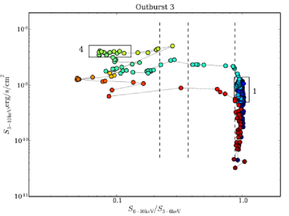
Figure 4: The two best covered outbursts of GX339-4. top: Detailed light curves and X-ray colour plots; bottom: HIDs of the two main outbursts. For clarity the errorbars are only shown in the flux and X-ray colour light curves rather than on the HID. On the HIDs we show the line tracking GX 339-4 from observation to observation. The colour scale is the date since the beginning of the outburst, blue is early and red is late. The boxes in the bottom diagrams show the selected outbursts for the spectral stacking described in Section 7 and shown in Fig 5. The number of the box corresponds to the number of the spectrum shown in Fig.5. The dotted vertical lines show the X-ray colours adopted for the state transitions outlined in Section 3.

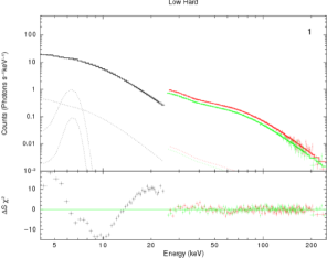
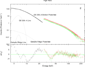
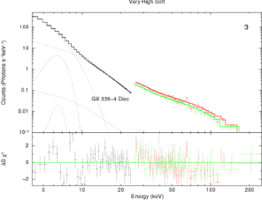
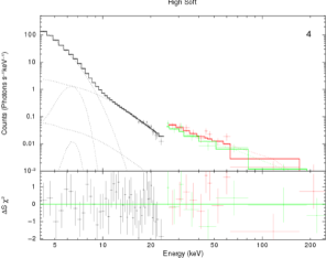
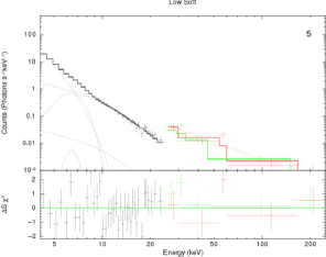
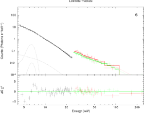
Figure 5: The spectra and model fits to the summed spectra. The fits are for those models which have been used in the automated fitting of the individual spectra, except for the Low Intermediate state, where the discbb+powerlaw model is shown. The more complicated models detailed in Table 2 are not shown here. The locations in the HID from where the spectra were taken are shown in Fig. 4, and are also indicated by the numbers in the top right corner of each spectrum. The data have been binned for the clarity of the plots alone (no binning was done prior to fitting) so that the significance of each data point is at least $3\sigma$. The effect of the binning is most obvious at the high energy end of the HEXTE spectra as well as the shorter exposure time data.

4 The Two Major Outbursts

We give a short summary of the major features of the two main outbursts of GX 339-4. Most of the observations in the rest of this study (424/634) come from these two outbursts. The detailed lightcurves, along with the X-ray colours and HIDs are shown in Fig. 4. Outburst 2 reaches its peak flux on the initial rise. There is a small decay as GX 339-4 evolves into the soft-state, and then the flux rises again to the same maximum flux. After this there is a gradual decay in flux. A detailed analysis of this outburst is given in Belloni et al. (2005).

In Outburst 3 the initial peak in the flux is almost an order of magnitude below the eventual maximum of the outburst. GX 339-4 remains in the hard state for over 100 days after this first peak, with the flux falling by a factor of two, then GX 339-4 rapidly moves into the soft-state. The flux continues to increase once in the soft state, and spectrum hardens fractionally. After the break in the light curve, by which time GX 339-4 is back in the soft state, the spectrum hardens before the flux falls and GX 339-4 rejoins the hard branch. This motion can be traced from the change in colour of the points in the HIDs shown in Fig. 4. A detailed analysis of the early part of this outburst is given in Belloni et al. (2006).

It is clear that Outbursts 2 and 3 reach different peak fluxes on the hard branch (see Fig. 4). Even though there are only a few observations, Outburst 4 also appears to peak at similar fluxes to that of Outburst 2 (see Fig. 1. Outburst 1 is insufficiently well sampled to be able to comment on its peak flux. On the return to the hard branch, all of the outbursts are at very similar fluxes, as noted by Maccarone (2003) for black hole X-ray binaries in general. It is possible that Outburst 3 is a factor 2 higher, but the offset is small compared to offsets in the flux of the intermediate states for each outburst.

The variation of the X-ray colour during Outbursts 2 and 3 is similar even though they occur two years apart. The change in X-ray colour with the outburst is shown again in Fig. 6, rescaled so that the beginning and end of the transition to and from the soft state are aligned. The “stretching factor”, the relative lengths of the two outbursts, is around $4:3$ for Outburst 2 to Outburst 3. The two curves are remarkably similar - the rise in flux and associated hardening just before halfway through an outburst occurs in both. There is also a suggestion that the temporary softening of the spectrum as GX 339-4 hardens again, which is clearly seen in Outburst 2, is also present in Outburst 3. This dip is also seen in the tail end of Outburst 4 when matched to the previous outbursts.

We investigated whether disc components could be present in observations where individual spectra were unable to indicate any significant disc component in the intermediate and hard states. We selected six areas of similar X-ray colour and flux from the HIDs of these two well observed outbursts corresponding to low hard, high hard, very high soft, high soft, low soft and low intermediate states (see boxes in Fig. 4). These areas were selected to cover a range in states, but also where there were a concentration of observations at a similar epoch. We sum the PCA and HEXTE spectra and associated backgrounds and refit the same sets of models as before in xspec (see Fig 5 for the spectra and the Appendix for the numerical results of the fitting).

The soft states are, unsurprisingly, well fit by a discbb + powerlaw model. The best fit model to the intermediate state spectrum is also a discbb + powerlaw model. We note that this is different to the best fit model of some of the individual spectra which make up this summed spectrum (compare Figs. 2 and 4). The improvement in $\chi^{2}$ is small, but significant as the degrees of freedom remain the same. We therefore conclude that the improved signal-to-noise of the summed spectrum allows an accurate fitting of the disc and so this model wins out over a purely broken powerlaw model. The low intermediate summed spectrum was constructed from observations of GX 339-4 as the outburst decayed, and as such a faint disc would be expected in this state. The disc temperature does, however, appear to rise relative to the soft state rather than fall as would be expected (see Section 6 for more details).

Both summed spectra from the hard state are poorly fit by the simple absorbed broken powerlaw model. The high flux of GX 339-4 during the observations or the long equivalent exposure of the summed spectra has resulted in very high signal-to-noise. Consequently the simple model is no longer a good fit to the data. An improved, but by no means good, fit to the data is achieved by introducing another break in the powerlaw slope as there is indication for this in the HEXTE data. We also added in a discbb model just in case a disc were present and detectable in these high quality spectra. There was no improvement to the fit in the low hard state (which is taken from observations on the rise of the outburst). In the high hard state, however, adding a disc improved the fit (see notes for Table 2).

The summed spectra do show disc components when they are not significantly detected by all the individual observations. This study can therefore not shed much light on the rise or fall of the disc in the hard state of GX 339-4. However, in long exposure observations in the high hard state, the fitted disc is at higher disc temperatures than what is observed in the soft state.

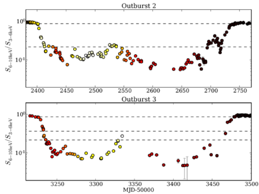
Figure 6: The variation in X-ray colour as the outbursts progress for the two major outbursts observed by RXTE. The date scale as been adjusted to align the beginning and end of the outbursts. The colour scale is that of the $3-10{\rm\thinspace keV}$ flux of GX 339-4, white for high flux and black for low flux. The colour scales have not been adjusted to match between the two plots. The dotted lines show the X-ray colours adopted for the different state transitions outlined in Section 3

Yu et al. (2007) show that the peak hard state flux of an outburst depends on the length of time since the previous outburst of GX 339-4. Using the detailed light- and X-ray colour-curves from the four outbursts observed by RXTE. The duration of Outbursts 2 and 3 (their Outbursts 6 and 7) appear to correlate with the length of time since the previous outburst (see Table 1). However Outburst 4 lasts longer than would be expected from the previous two and also reaches the same peak flux as Outburst 2 without such a long period of quiescence preceding it. Under the assumption that the duration of the outburst is linked to the “waiting time” by a power-law relationship, then Outburst 4 would be expected to last around 280 days (Outburst 4 was not in the study of Yu et al., 2007). However, the end of the outburst is well monitored by RXTE and there are sufficient observations at the beginning to rule out a much earlier start (a mis-measurement of 100 days would be required to match the relation obtained for the other outbursts) or a lower peak flux.

The length of the outburst, however, would depend on how quickly the material in the disc was drained during the outburst as well as the amount of material which has built up in the disc since the last outburst . Under the assumption of a constant deposition rate of material into the disc and that the disc is completely emptied during each outburst, then the interval is a measure of the amount of material which could contribute to the outburst. In reality the disc is unlikely to be totally emptied during each outburst.

As is clear from Table 1, the length of the outburst, $t_{\rm outburst}$, does not correlate well with the interval between outbursts, $t_{\rm prior}$. However, the duration of an outburst depends not only on the amount of material in the disc, but also on the rate at which it is depleted. The peak X-ray flux is likely to be a good measure of the depletion rate within the outburst. If we correct the interval between outbursts by dividing by the X-ray flux, we obtain values which do correlate with the length of the outburst, $\mathcal{L}$. We note that we only have four outbursts and hence three estimate on the relative magnitudes of the durations of the outbursts to use in this study.

Table 1: Outburst Durations

OB	Start	Stop	$t_{\rm outburst}$	$t_{\rm prior}$	Peak Flux	$\mathcal{L}$
	MJD-50000		days	days	(${\rm\thinspace erg~{}s^{-1}~{}cm^{-2}}$)
1	800	1240	440	-	$2.7times10^{-9}$	-
2	2400	2730	330	1160	$9.4\times 10^{-9}$	123
3	3225	3475	250	495	$5.0\times 10^{-9}$	99
4	4130	4240	110	655	$9.7\times 10^{-9}$	68

The start and stop times for the outbursts are taken as the departure and return to the hard state (X-ray colour = 1). The separation is then the time between the return to the hard state for one outburst on its decline and the departure from the hard state on the subsequent outburst on its rise.

5 Iron Line

An $F$-test in combination with the line normalisation (see Section 3 for more details) were used to test for the presence of an emission line (assumed to be the iron $K_{\alpha}$ fluorescence line) at $6.4{\rm\thinspace keV}$. However out of 628 spectral fits, 400 require a line, and these occur all over the HID, in all states.

We did investigate the effect of allowing the line energy to be free, between $6-7{\rm\thinspace keV}$. However this caused some erroneous fitting, mainly in cases where there is some slight curvature to the low energy powerlaw. The curvature is a broad feature usually at lower energies than $6{\rm\thinspace keV}$. In trying to fit this feature, the gaussian component became very broad and “pegged” at the lower energy limit with a large uncertainty in the line energy, even though the residuals showed clear excesses in the $6-7{\rm\thinspace keV}$ range. Selecting these models with a significant “line” detection as the best fitting would not give information about any line present as this has not been fitted by the gaussian. Therefore, any line component, even if deemed significant by the $F$-test which had an energy uncertainty of $>1{\rm\thinspace keV}$ was taken not to be representing a line, but another continuum component, and so the line “detection” was discarded from further analysis. In some cases a line was well and sensibly fit at energies different from $6.4{\rm\thinspace keV}$, however these were few. However, this method discards observations where a line may be present but xspec has preferentially fitted the curvature in the powerlaw instead. We therefore present the results on the analysis with a gaussian component fixed at $6.4{\rm\thinspace keV}$ in this section. We note that using the most stringent cut-off in the $F$-test when selecting lines when their energy was free did show a variation in the energy across the HID. The lowest energy was at the top of the low-hard state and the highest energy was in the intermediate state at the end of an outburst, during the return to quiescence.

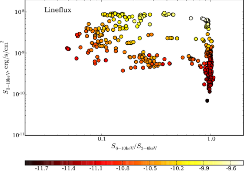
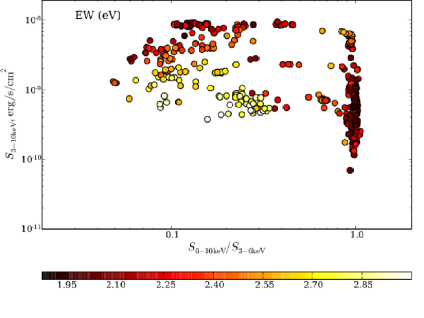
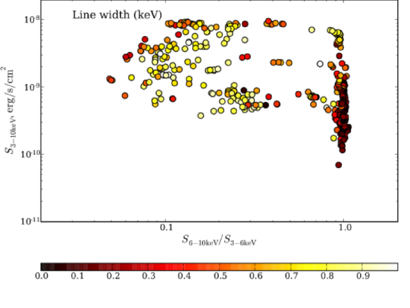
Figure 7: The hardness-intensity diagram from all the observations where a significant line is detected. top The colour scale is from the line flux. The decrease in line flux during the course of the outburst is clearest at the low soft states. middle The colour scale is for the equivalent width of the iron line (logarithmic, eV). In some cases the calculated equivalent width was greater than $1{\rm\thinspace keV}$ and these have been truncated in the colour scale to aid clarity. bottom The colour scale is for the line width in ${\rm\thinspace keV}$.

We extract the line flux over a $0.1-10{\rm\thinspace keV}$ range. The line is strongest at the highest fluxes in the hard state, see Fig. 7, whereas the EW is largest at the lowest flux soft states. The line width is also largest in the soft state (Fig. 7). Fitting the line flux against the $3-10{\rm\thinspace keV}$ total flux shows a relationship for all of the data of

$$S_{\rm 0.1-10,line}\propto S_{\rm 3-10{\rm\thinspace keV}}^{1.07\pm 0.02},$$

however there is a large scatter of around the best fitting line (see Fig 8). The Spearman Rank correlation coefficient is $0.860$. We also calculate the Kendall’s Tau correlation coefficient, $0.678$. The variance of the latter is $0.0011$ and so the significance of the correlation is $20.2\sigma$. As the continuum increases, then the line does in an almost linear relationship. However, the X-ray colour of GX 339-4 for each observation shows that the hard and soft states have different behaviours.

We split the data into extremely soft (X-ray colour $<0.22$) and hard (X-ray colour $>0.87$) states and refit the correlation. The hard and soft state correlations for both the $7-20{\rm\thinspace keV}$ and $3-10{\rm\thinspace keV}$ fluxes are then

$$S_{\rm 0.1-10,line} \propto S_{\rm 3-10{\rm\thinspace keV}}^{1.24\pm 0.02}\quad{\rm hard}$$

$$S_{\rm 0.1-10,line} \propto S_{\rm 3-10{\rm\thinspace keV}}^{0.57\pm 0.06}\quad{\rm soft}$$

$$S_{\rm 0.1-10,line} \propto S_{\rm 7-20{\rm\thinspace keV}}^{1.13\pm 0.03}\quad{\rm hard}$$

$$S_{\rm 0.1-10,line} \propto S_{\rm 7-20{\rm\thinspace keV}}^{0.70\pm 0.03}\quad{\rm soft},$$

respectively (see Fig 8). We also show the correlations of the $7-20{\rm\thinspace keV}$ total flux with the line flux, following Rossi et al. (2005), as only photons with energies $\gtrsim 7{\rm\thinspace keV}$ are be able to ionise iron. We do not, however, fit all observations with a single line as there are clearly two separate relations in the $7-20{\rm\thinspace keV}$ flux in Fig. 8

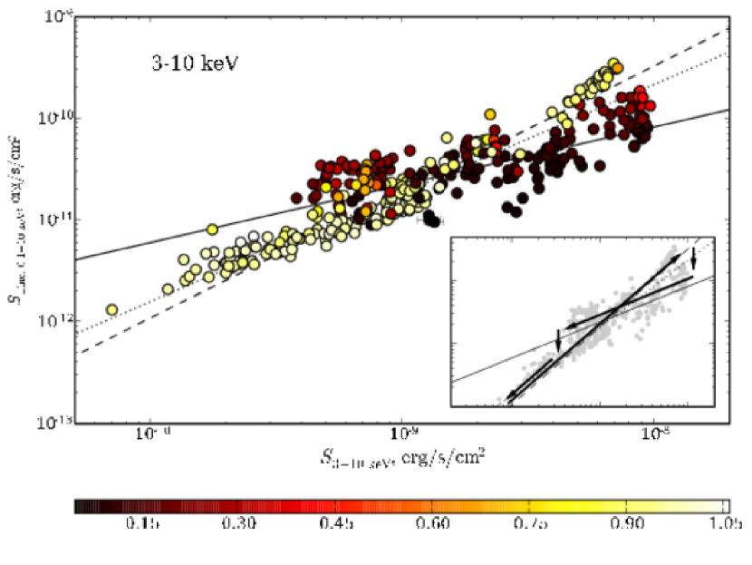
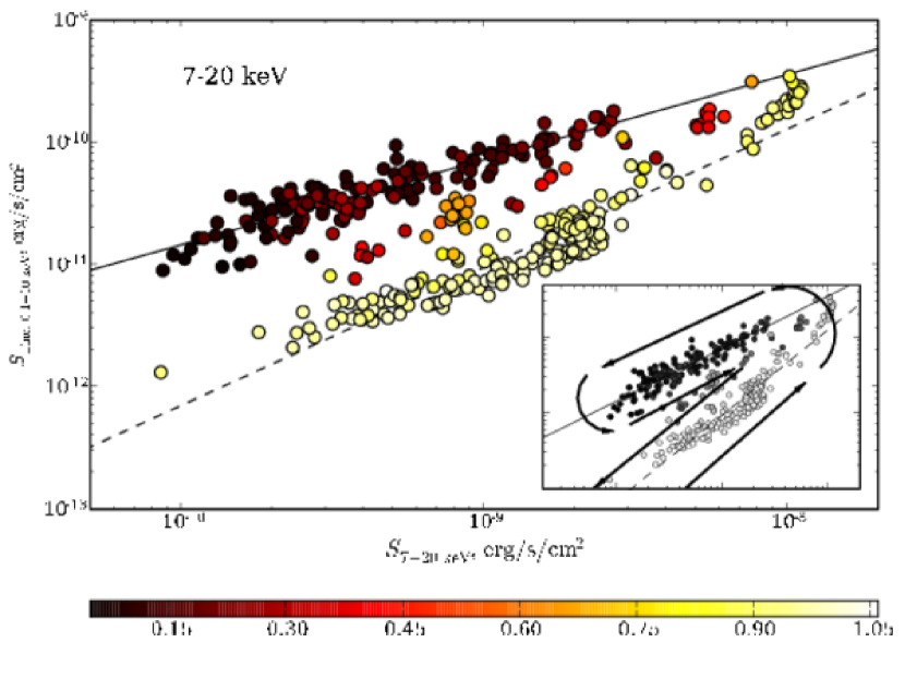
Figure 8: The flux of the $6.4{\rm\thinspace keV}$ iron line as a function of top the $3-10{\rm\thinspace keV}$ total flux and bottom the $7-20{\rm\thinspace keV}$ total flux. The colour scale on the plot is the X-ray colour of the observation. The best fit relation is to all the data is shown by the dotted line. The best fit to the soft and hard states are shown by the black solid and dashed lines respectively. The insets show the approximate motion of GX 339-4 through the diagrams during an outburst.

In both flux bands, the slope of the relation of the line flux is different between the soft and hard states. In the $7-20{\rm\thinspace keV}$ flux band, the powerlaw is the dominant spectral component being probed. The powerlaw flux falls away during the soft state and, noting that the lineflux remains approximately constant across all X-ray colours in Fig. 7, the soft state points have been displaced to the left. However using the lower energy $3-10{\rm\thinspace keV}$ band, the disc is the dominant spectral component in the soft state, but the powerlaw takes it’s place in the hard state. Therefore there is no sideways displacement of the soft state points relative to the hard state.

The difference between the behaviour of the line fluxes in the hard and the soft state could arise from changes in the ionization parameter as well as from differences in the spectral slope of the incident radiation. The X-ray spectrum above $7.1{\rm\thinspace keV}$ of a soft state object is steeper than that of a hard state object. Thus, there are more lower energy photons available to ionize the iron in the soft state compared to the hard state. As the cross-section of the ionization process decreases with increasing photon energies, a soft state is therefore more efficient to produce the iron line than a hard state for a given 7-20 keV flux. Additionally to this effect a soft state may have a smaller ionization parameter, which would also increase the observed line flux (for more details see e.g. Reynolds & Nowak, 2003).

5.1 X-ray Baldwin Effect

Having detected lines in most of observations at different states during out an outburst we investigated whether there is an X-ray Baldwin effect in GX 339-4. Baldwin (1977) found that the equivalent width of the Civ line decreased with increasing UV luminosity in a sample of AGN. An X-ray Baldwin effect has been reported in AGN by a number of authors (Iwasawa & Taniguchi, 1993; Nandra et al., 1997; Page et al., 2004; Bianchi et al., 2007; Mattson et al., 2007). They find that the equivalent width depends on the luminosity in the following range

$$EW\propto L^{\beta},$$

where $-0.20\leq\beta\leq-0.14$.

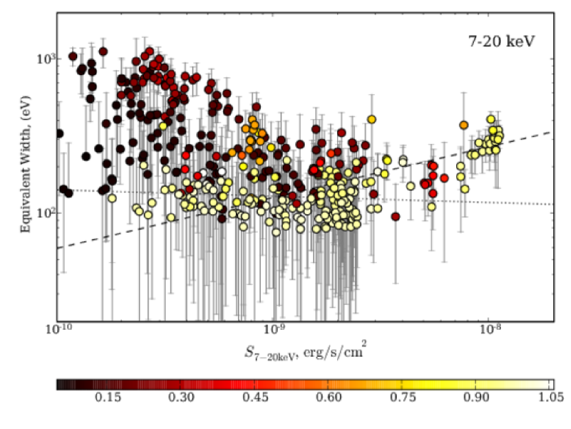
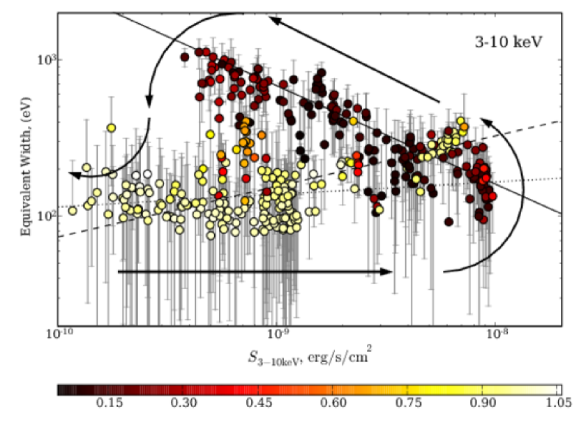
Figure 9: The Equivalent Width of the Iron line against the flux during the outbursts, top: $7-20{\rm\thinspace keV}$ flux, bottom: $3-10{\rm\thinspace keV}$ flux. The colour scale shows the X-ray colour of the spectrum for each observation, black being soft and white being hard. The solid line shows the best fit to the soft state, the dashed line the best fit to the hard state, and the dotted line to the low-flux hard states. The arrows indicate the motion of GX 339-4 through the diagram during an outburst.

The equivalent width was calculated during the course of the fitting, and is shown on the HID in Fig. 7. The HID clearly shows that, on average, the equivalent width is highest in the softest and lowest flux states. Fig. 9 shows the equivalent width of the iron line against the flux of the observation, with the X-ray colour of the spectrum as a colour scale. The two states (hard and soft) appear to have different correlations between the flux and equivalent width. Extracting those observations which have an X-ray colour of $<0.22$ (the extreme soft state), the best fit to the anti-correlation is,

$$EW\propto S_{3-10{\rm\thinspace keV}}^{-0.61\pm 0.09}$$

$$EW\propto S_{7-20{\rm\thinspace keV}}^{-0.55\pm 0.05},$$

with Spearman Rank correlation coefficients of $-0.840$ and $-0.430$ respectively. The Kendall Tau are $-0.644$ and $-0.308$, with significances of $10.6\sigma$ and $5.07\sigma$ respectively. We also take the hard state observations (those with X-ray colours $>0.87$) we fit the observations with

$$EW\propto S_{3-10{\rm\thinspace keV}}^{0.32\pm 0.07}$$

$$EW\propto S_{7-20{\rm\thinspace keV}}^{0.33\pm 0.02},$$

with Spearman Rank correlation coefficients of $0.262$ and $0.237$ respectively. The best fitting line has a positive index. However this is the result of the combination of the large scatter in the majority of the hard state points and the small cluster at high fluxes, separate from the rest. If we ignore those points with $S>2\times 10^{-9}{\rm\thinspace erg~{}s^{-1}~{}cm^{-2}}$ and $EW>400{\rm\thinspace eV}$, and fit the bulk of the hard state observations, we find $EW\propto S_{3-10{\rm\thinspace keV}}^{-0.09\pm 0.14}$ and $EW\propto S_{7-20{\rm\thinspace keV}}^{-0.04\pm 0.04}$ , shown as the dotted line in Fig. 9. These are consistent with no change in the EW with flux. No errors in the $7-20{\rm\thinspace keV}$ fluxes could be obtained from xspec and so the uncertainties in the slopes for the $7-20{\rm\thinspace keV}$ fluxes only include the errors in the EWs. The uncertainties in the slope of the $3-10{\rm\thinspace keV}$ fits include the errors from the EWs and the fluxes.

If the lineflux decreases at the same rate as the continuum then the measurable equivalent width of the line decreases as the flux decreases. This effect would therefore lead to a lower cut-off for the minimum measurable equivalent width with flux with a negative slope. This would result in a small slope in the data points, whereas it should be flat. We therefore do not believe that there is an X-ray Baldwin effect in GX 339-4 in the hard state.

The motion of GX 339-4 through the flux-equivalent width plane is that at the beginning of the outburst the flux increases at constant equivalent width. At the peak flux, when the source moves into the soft state, the equivalent widths start to increase as the flux decreases. When the source returns to the hard state, the equivalent widths reduce suddenly and then become constant as the flux falls (see arrows in Fig. 9). This is another example of hysteretical behaviour from GX 339-4.

There is an X-ray Baldwin effect in the $6.4{\rm\thinspace keV}$ iron line in the soft state of GX 339-4. The slope of the relation, however, is much steeper than that observed in AGN. Iwasawa & Taniguchi (1993) studied Seyfert 1s and quasars, whereas in a sample of 53 AGN from the XMM-Newton archive, Page et al. (2004) used 14 radio loud and 39 radio quiet sources. Bianchi et al. (2007) excluded radio loud objects from their complete study of radio quiet Type 1 AGN in the XMM-Newton archive. These studies all show an X-ray Baldwin effect between a variety of sources, rather than an intrinsic effect within one source. Most of the AGN in studies of the X-ray Baldwin effect have been radio quiet AGN, analogous to the soft state of black hole X-ray binaries. Scaling the effect described here for GX 339-4 up to AGN would result in an effect which occurs on very short timescales.

5.2 Links to the Powerlaw Slope

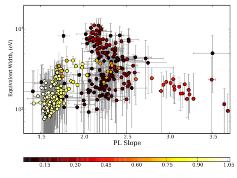
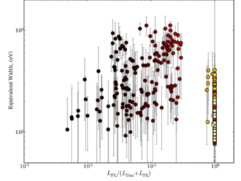
Figure 10: top: The equivalent width against the power law slope. The colour scale shows the X-ray colour of the spectrum for each observation, black being soft and white being hard. The plot has been truncated at $\Gamma=1.4$ and $\Gamma=3.5$, and $\Gamma$ outside of this range is unlikely to be an accurate description of the data. bottom: The disc fraction of GX 339-4 against the equivalent width with the colour scale representing the X-ray colour. See Section 7 for more details about the disc fraction.

In a recent study of 12 Seyfert 1 and 1.2 galaxies, Mattson et al. (2007) fitted RXTE data with a pexrav model, which simulates an exponentially cut-off power-law reflected by neutral matter, and a Gaussian line. They find a positive correlation between the line equivalent width and the underlying power law slope for $\Gamma<2$. For $\Gamma>2$ they found an anti correlation, with a peak equivalent width of $\sim 250{\rm\thinspace eV}$, see their Figs. 1a and 3. We plot the powerlaw slope (below the break in the case of a broken powerlaw) against the equivalent width for GX 339-4 in Fig. 10. We note that superficially the shape of the distribution is very similar, however there is a larger scatter in the shape of the distribution. The colour scale corresponds to the X-ray colour of the observation. The correlation corresponds to the hard state whereas the anti-correlation corresponds to the soft state.

In GX 339-4 the hard state, which usually associated with the presence of a steady, mildly relativistic jet, is found at the low $\Gamma$s. In Mattson et al. (2007) the low $\Gamma$ end of relation is dominated by points from 3C 273. The positive correlation is composed of observations of radio loud Seyfert 1 galaxies, the peak by radio quiet Seyfert 1s, and radio quiet Seyfert 1.2s comprise the anti-correlation part of the relation. In GX 339-4, the soft, disc dominated state is mostly at the peak of the relation with the intermediate state at the high $\Gamma$ end.

The model of an X-ray binary outburst presented in Fender et al. (2004) indicates that the jet is quenched as the disc becomes dominant in the soft state. As the jet is the source for the radio emission, when this quenches, the X-ray binary becomes radio quiet, in the soft state, as shown in Fig. 16. We therefore would expect to see observations of the soft, radio quiet state of GX 339-4 on the negative correlation and the hard, radio loud state on the positive correlation from this model.

George & Fabian (1991) simulated the spectrum expected from an X-ray source which illuminates a slab and showed that it should include an iron line and a “Compton hump.” As the spectrum softens ($\Gamma$ increases) there are fewer photons with enough energy to photo-ionise iron, and so the iron line EW decreases. This is observed in the soft state of GX 339-4 as well as in the sample in Mattson et al. (2007).

Mattson et al. (2007) suggest that for $\Gamma$ to increase as the jet dominance decreases the jet would have a hard X-ray component associated with it. On the other side of the relation, observations of MCG–6-30-15 have shown that the reflection component remains relatively constant (Miniutti et al., 2007), so when $\Gamma$ increases the EW decreases.

As the relations between the power-law slope and the equivalent width of the iron line are similar for GX 339-4 and the sample of AGN it is reasonable to assume that the processes at the centre of an AGN and an XRB are similar. As XRBs have radio (jet) dominated quiescent periods and disc dominated outbursts, then this similarity in the relations points towards to AGN also having outburst phases. As the black hole masses in AGN are $\sim 10^{5}-10^{8}$ times larger, their outburst phases are much longer. However, this result indicates that the path of an AGN through an HID would be similar to XRBs, though their direction is currently unknown. The AGN HID would have to be constructed so that ultra-violet emission from the disc would be included. This is further discussed in Section 7.

As the hard, intermediate and soft state points appear in different locations in the diagram, we reform the relation using the disc fraction (see Section 7 and Fig. 10). The X-ray colour is indirectly related to the disc temperature and luminosity. The disc fraction, however, is a more physical quantity describing the relative luminosities of the disc and the powerlaw components of the spectrum. The hard and intermediate state appear with no disc fraction as the best fitting model contains no disc component. The soft states occur over a range of disc fractions and equivalent widths. We split the observations into two sets; those with a disc (disc fraction $<0.5$) and those without (disc fraction $\geq 0.5$) and perform a t-test to indicate whether the means are significantly different and also a K-S test to see if the two distributions of equivalent width are drawn from the same population. The probabilities for both tests show that the two data-sets have the same mean/were drawn from the same population are very low ($P_{KS}=1.29\times 10^{-25}$ and $P_{t}=1.3\times 10^{-46}$ respectively). We therefore conclude that, although the separation of the two populations is small, the behaviour of the equivalent width of the line is different when GX 339-4 is in outburst to when it is in quiescence/the hard state. However the difference in behaviour is less clear in this presentation of the variation of the equivalent width with the state of GX 339-4.

6 Disc Temperature

Selecting those observations where a disc is present we extract the disc temperature. The variation in disc temperature through the HID is shown in Fig. 11. The highest disc temperatures are observed at the highest fluxes in the soft state, and the lowest temperatures at the lowest fluxes. The variation through the soft state is smooth, even though we show data from all four outbursts. The observations with an X-ray colour $>0.4$ show a disc temperature much higher than those in the soft state (though the colour scale is truncated at $1{\rm\thinspace keV}$). In fact they appear to indicate that the disc temperature is rising as the source is fading down the hard branch. As stated in Section 3.2 it is unlikely that these disc “detections” are true. Without spectral information below $3{\rm\thinspace keV}$ we are limited to how accurately we can determine the presence or absence of a disc. If there is any curvature in the spectrum, this will be better fit by a higher temperature disc combined with a powerlaw rather than a simple powerlaw. However, the curvature may not be the result of a disc component, and as we have on purpose restricted the choice of models to a limited range, the disc turns out to be the statistical best fit. The temperature of these disc fits is much higher than would be expected for a decaying disc ($>1{\rm\thinspace keV}$). If these are true discs, then the temperature at the end of an outburst doubles over 10-20 days compared to the gradual $\sim$250 day decay in the soft state. Also, as the fluxes of these disc components is $10^{-11}-10^{-10}{\rm\thinspace erg~{}s^{-1}~{}cm^{-2}}$ rather than the $10^{-9}-10^{-8}{\rm\thinspace erg~{}s^{-1}~{}cm^{-2}}$ for the soft-state disc detections, we conclude that the diskbb model is not fitting the true disc component. We do not include any of these points in any analysis in this section.

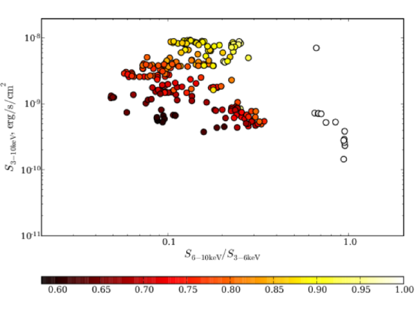
Figure 11: The hardness-intensity diagram from all the observations where a disc is detected. We do not consider the apparent detections of the disc in the hard state as true detections. The colour scale is for the disc temperature in keV, and has been truncated at $1{\rm\thinspace keV}$ to emphasise the variation in disc temperature during the soft state.

The spectrum of an optically thick, geometrically thin accretion disc is the result of a sum of black-body spectra, one for each radius - a so-called multi-coloured disc model. The maximum temperature for such a disc should occur close to the inner edge of the accretion disc, $R_{\rm in}$. In a similar way to the Stefan-Boltzmann law, the resulting disc flux should follow:

$$S_{\rm Disc}\propto R_{\rm in}^{2}T^{4},$$

mimicking the emission from a black body whose radius is that of the inner edge of the disc and whose temperature is that of the disc at the innermost radius. In the first instance we assume a constant inner radius for the disc. We initially assumed that in the soft state, the flux from the disc would dominate the total flux to such an extent that this relation would hold for the total flux received from GX 339-4 and hence expected that $S_{3-10{\rm\thinspace keV}}\propto T^{4}$.

Fitting the correlation of the total flux from GX 339-4 with the disc temperature (for disc temperatures $<1{\rm\thinspace keV}$), we obtain

$$S_{3-10{\rm\thinspace keV}}\propto T^{9.44\pm 0.12},$$

which is steeper than what is expected and is shown by the dashed line in Fig 12 top. Our assumption that the flux is dominated by the disc component is unlikely to be true. We see extra flux above what would be expected from the disc alone at the lower flux observations. As a result we need to use the unabsorbed disc flux. There are two methods of obtaining the disc flux from the fit; direct from xspec by setting the normalisations of all other emission components to zero (including the absorption) or calculating it from the fitted normalisation and temperature of the diskbb model. The advantage of using the second method is that the uncertainties on the disc flux are able to be estimated using error propagation, and so this method is used for the remainder of this work.

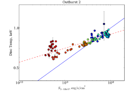
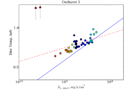
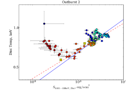
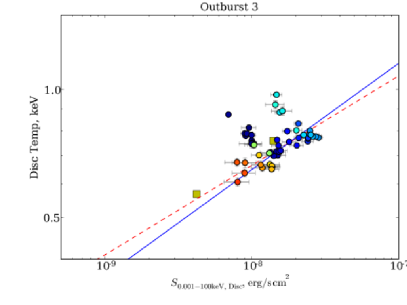
Figure 12: For Outburst 2 (left) and Outburst 3 (right): The X-ray flux against the disc temperature (top) and the disc flux against the disc temperature for the two main outbursts of GX 339-4 (bottom). The colourscale shows the time since the transition into the soft state - blue is early, red is late. The best fit lines are shown by the dashed line ($T^{9.44}$ for the flux plots, and $T^{4.75}$ for the disc flux plots – from the observations with X-ray colour$<0.2$). The expected correlation of $S_{\rm Disc}\propto T^{4}$ is shown by the solid line. The points off the top left of these plots are the observations in the hard state which appear to require discs. The square points are measurements from Miller et al. (2004b, a, 2006).

However, the decay in the disc temperature as the disc flux decreases is consistent with the model of $S_{\rm Disc}\propto T^{4}$ as shown by the lines in Fig. 12. The square points are from Miller et al. (2004a, b, 2006), some of which fall outside the limits of this diagram. These points are consistent with $T^{4}$ and the highest temperature one ($0.76{\rm\thinspace keV}$) also matches the the set of values we obtain (see also Fig. 13).

Although we plot both major outbursts here, the decay is clearest in the first one as there is a “clean” decay in flux with only a small variation in X-ray colour while in the soft state (Fig. 4). The flux decays slightly when the GX 339-4 reaches the soft state. There is a small rise and hardening of the spectrum before the GX 339-4 returns to the soft state and the flux and disc temperature decay gradually. The entry and exit from the soft state are seen as “spurs” off the $T^{4}$ relation (Fig. 12). These may be artifacts of the fitting process and result from the limitations of the PCA bandwidth.

Once the second outburst has reached the soft state, the flux rises at a fairly steady X-ray colour and then the spectrum hardens. After a gap in the light curve the X-ray colour remains relatively steady as the flux decays. Both the entry into and departures from the soft state (in the middle and at the end of the outburst) are seen as “spurs” off the rest of the points, which scatter neatly around the $T^{4}$ relation. At face value, the implication of these “spurs” is that the disc cools onto the $T^{4}$ relation, and at the end of the outburst heats up again. This increase in the disc temperature as GX 339-4 returns to the hard state is also seen in the summed spectra in Section 4.

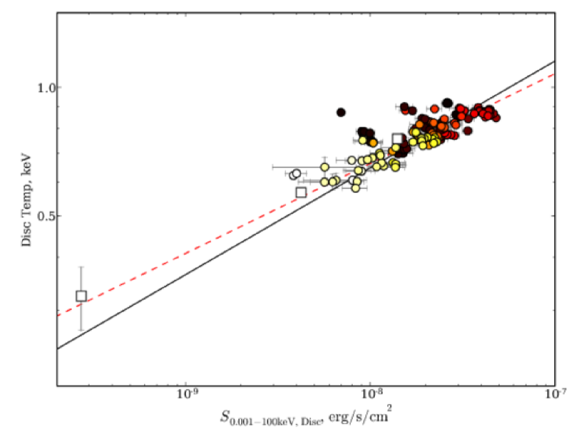
Figure 13: The Disc Flux and Disc temperature for observations with an X-ray colour of $<0.2$. The x-axis has been extended to show all the points from Miller et al. (2004b, a, 2006) in white squares. The black solid line is the theoretical $T^{4}$ relation and the red dashed line is the best fit line to these observations $T^{4.62}$. The colour scale shows the date since the first detection of the disc in the continuum emission.

All of the points outside of the general scatter around the $T^{4}$ relation are from the observations which have a disc but are in the intermediate state. Selecting observations with X-ray colours $<0.2$ and disc fluxes of $S_{\rm Disc}>5\times 10^{-9}{\rm\thinspace erg~{}s^{-1}}$ retains only those which scatter close to $T^{4}$ (see Fig. 13). Fitting these we obtain a best fit of

$$S_{\rm Disc}\propto T^{4.75\pm 0.23}.$$

with a Spearman Rank correlation coefficient of $0.904$ and a Kendall Tau of $0.740$ with a significance of $23.6\sigma$ (taking into account the errorbars in the disc temperature and the disc flux). Although this is still steeper than the theoretical expectation, the theoretical expectation still is still a good “by-eye” fit. The range of disc temperatures is only just under a factor of 2 and the flux a factor of 10, and so the correlation can easily be masked by the scatter.

6.1 Disc Radii

If the theoretical relation is applicable, then if the inner radius of the accretion disc is constant, the temperature should follow a $T^{4}$ law. The diagrams show that when in the softest part of the soft state, the temperature variation is as expected. Therefore we expect that the inner radius of the disc is constant. The inner radius of the accretion disc can be calculated from the normalisation of the xspec model;

$$R_{\rm in}/R_{\rm G}=0.677\frac{d_{\rm 10{\rm\thinspace kpc}}}{M/M_{\odot}}\sqrt{\frac{\kappa}{\cos i}},$$ (1)

where $\kappa$ is the normalisation of the disc model in xspec and $i=30^{\circ}$ is the inclination of the system. The distance to GX 339-4 is taken to be $8{\rm\thinspace kpc}$ (Zdziarski et al., 2004) and the mass as $10M_{\odot}$. We do not include any uncertainties from the distance and mass into the calculation of the uncertainties of $R_{\rm in}$. The variation in the inner radius of the accretion disc during the two outbursts are shown in Fig. 14 top. During the part of the outburst where the temperature follows a $T^{4}$ law, the inner radius of the disc is constant within the uncertainties. The disc behaves as a standard thin accretion disc during these parts of the outburst.

However, the same observations which show a departure from $T^{4}$ also show a change in the inner radius of the disc. The implication of these points is that the disc recedes outwards to something like the innermost stable orbit at the beginning of the outburst, and falls inwards at the end. This is obviously not a physical explanation or model for the outburst, and so either the model adopted for the emission from the disc is not appropriate or the spectral analysis is insufficiently detailed to investigate the disc in the intermediate states.

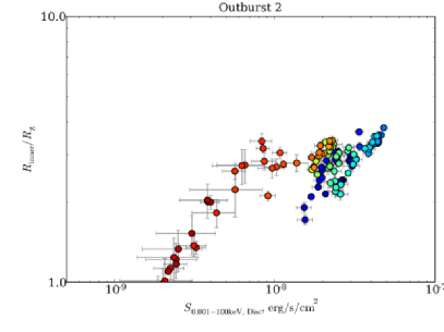
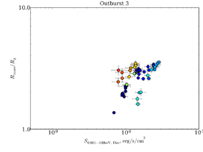
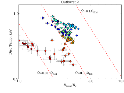
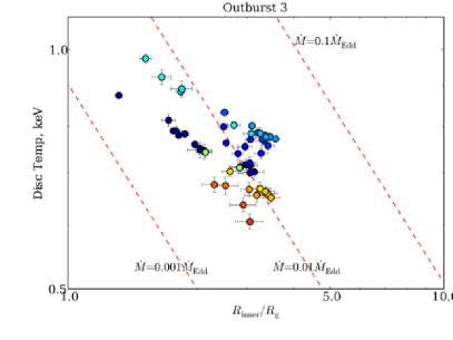
Figure 14: For Outburst 2 (left) and Outburst 3 (right): top: The inner radius of the disc in units of $R_{\rm g}$ through the outburst. bottom: The evolution of the temperature of the disc at the inner radius with the inner disc radius. The dotted lines correspond to different constant disc accretion rates. The colour scale shows the time since the transition into the soft state - blue is early, red is late.

We follow the analysis of GRS 1915+105 in Belloni et al. (2000) and plot simple derivatives of the two measured and independent quantities, $T$ and $R_{\rm in}$ (see Fig. 14). It is in principle possible to calculate the accretion rate from each spectrum using the expressions from a standard thin disc,

$$\dot{M}=\frac{8\pi R_{\rm in}^{3}\sigma_{\rm T}T^{4}}{3GM}$$ (2)

(e.g. Belloni et al., 1997). Therefore any given $R_{\rm in}$ and $T$ implies an accretion rate, and lines of constant accretion rate as a fraction of the Eddington limited rate where we assume an efficiency of the accretion flow, $\eta$, of 10 per cent. are shown in Fig. 14 bottom. The accretion rate is observed to rise at the beginning of the outburst, reaches a maximum when the state is at the highest soft flux, and then falls off. In both the outbursts shown here the peak accretion rate is approximately $0.03\dot{M}_{\rm Edd}$, where $\dot{M}_{\rm Edd}=L_{\rm Edd}/\eta c^{2}$. The observations which formed the spurs off the $T^{4}$ relation have a more rapid change in the accretion rate through the disc. Comparing these two diagrams with the equivalent one in Belloni et al. (2000), the slope of the observations in GRS 1915+105 are similar to that of the spurs in GX 339-4.

Gierliński & Done (2004) include a colour temperature correction factor in their analysis of discs in ten black hole binary systems, following Shimura & Takahara (1995); Merloni et al. (2000). The effect of this correction is almost always to harden the spectrum. For the same disc luminosity, adding in the colour correction increases the disc temperature. Therefore our results may be consistent with $\propto T^{4}$ if the temperature we extract from xspec includes a colour correction effect. To further investigate whether the relation is truly shallower than expected more data on the disc in the soft state is required. We note that McClintock et al. (2007) also find a deviation from the expected $T^{4}$ law in the X-ray Nova H1743-322 and Tomsick et al. (2005) present a detailed correlation between $L$ and $T$ with deviations from the expected relation for 4U 1630-47.

Comparing Figs. 7 and 11, as the disc temperature decreases, the equivalent width increases. Excluding the observations of the disc in the hard state and fitting the correlation gives

$$EW\propto T^{-3.3},$$

with a Spearman Rank correlation coefficient of $-0.704$ and a Kendall Tau of $-0.494$ with significance of $9.48\sigma$.

7 Disc Fraction Luminosity Diagram

In a study whose aim was to compare AGN and X-ray binaries, Körding et al. (2006) construct a more general version of the HID. The location of points in the HID depends on the total luminosity of the system and the strength of the non-thermal to thermal emission. In binaries, both the power-law and disc components are observed in X-rays, whereas in AGN the disc peaks in the UV band. As a result the HID for AGN as estimated from X-ray data alone would be unlikely to give any insight into the state of the source, and UV data from a large number of AGN is scarce.

Therefore Körding et al. (2006) generalised the HID by using the total luminosity and the disc fraction which is calculated from

$${\rm Disc\,Fraction}=\frac{L_{0.1-100{\rm\thinspace keV},\ {\rm PL}}}{L_{0.01-5{\rm\thinspace keV},\ {\rm Disc}}+L_{0.1-100{\rm\thinspace keV},\ {\rm PL}}}.$$

The Disc Fraction characterises the relative strengths of the disc and power-law components and also remains finite if either of the components approach zero.

We adapt this characterisation to the spectrum of GX 339-4. The model fits throughout the outbursts of GX 339-4 allow the disc and power-law fluxes to be calculated, $S_{\rm disc}$ from $0.001-100{\rm\thinspace keV}$ and $S_{\rm PL}$ from $0.1-100{\rm\thinspace keV}$. This allows us to calculate a Disc Fraction Luminosity diagram (DFLD) for an X-ray binary for the first time. To calculate the luminosity of the different components we take the distance to GX 339-4 to be at $8{\rm\thinspace kpc}$. The DFLD is shown in Fig. 15. The colour scale tracks GX 339-4 through the diagram during the outburst, and is linked to the time since the beginning of the outburst (similar to Fig. 4).

Körding et al. (2006) simulate a DFLD for 100 objects based on previous work on the evolution of the disc and power-law components during an outburst (see their Fig. 10). Reassuringly, even for only two outbursts from one object, Fig. 15 looks similar.

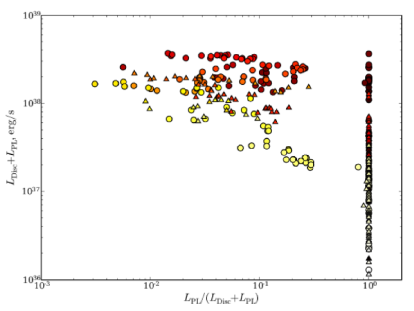
Figure 15: The Disc-Fraction Luminosity diagram for GX 339-4 for the two major outbursts. The colour scale shows the date of the observation relative to the start of the outburst - black is early, white is late. The Outburst 2 is shown by circles, Outburst 3 by triangles.

We note that as we only use X-ray observations in this study, this DFLD is limited, as in quiescence a disc is again seen. However, this disc is cooler, and so is best observed in the UV and it is not seen in the X-ray. This re-appearance of the disc is hinted at by the softening of the low flux hard state tail in the HID (Fig. 2). Future outbursts where the decays are studied in the Ultra-violet will reveal the shape of the DFLD for all states that XRBs exhibit.

The shape of the DFLD is subtly different to the HID. As the disc flux and temperature decay, the X-ray colour remains almost constant, before very rapidly hardening at the end of the outburst. This is a result of the X-ray colour being an indirect measure of the disc flux. The Disc Fraction is a more physical measure, and as a result the decay of the disc can be easily tracked as the disc fraction slowly reduces towards the power-law dominate state.

The tracks of the two outbursts through the DFLD is very similar to that in the HID. The hardening and softening of the spectrum is seen along with the decay in flux. However, the motion is more spread out. Whereas in the HID, the range in X-ray colour was from $0.03-0.3$ while the source was in the soft state, the range in the disc fraction is from $0.007-0.3$. This allows a more detailed investigation into the variation of the disc during an outburst.

There is a large gap in the diagram between the power-law dominated section and the area where a disc is detected. This is the result of the limited spectral coverage of the RXTE PCA. The gradual rise of the disc may be taken as the steepening of the lower slope in the broken powerlaw. Only once the curve of the black-body is dominant does the disc model become the best fitting, by which time the disc fraction is already significant.

8 Radio/X-ray Correlations

To investigate correlations of the radio flux within the DFLD the we took the compilations presented in Corbel et al. (2000) and Gallo et al. (2004). As the radio observations were not coordinated with the RXTE observations we match the two data-sets as best possible. If there is a radio observation within two days of an X-ray observation, then this radio observation is linked to the X-ray one. A two day overlap gave a reasonable number of X-ray observations which had corresponding radio flux values.

There was little data from MOST, nor from $2.3$ and $1.5{\rm\thinspace GHz}$ ATCA observations. As a result we concentrate on $8.5$ and $5{\rm\thinspace GHz}$ data as well as the spectral index, $\alpha$ (where $S_{\rm Radio}\propto\nu^{\alpha}$). The data from Corbel et al. (2000) cover Outburst 2, whereas the radio data from Gallo et al. (2004) cluster around the peak of Outburst 3.

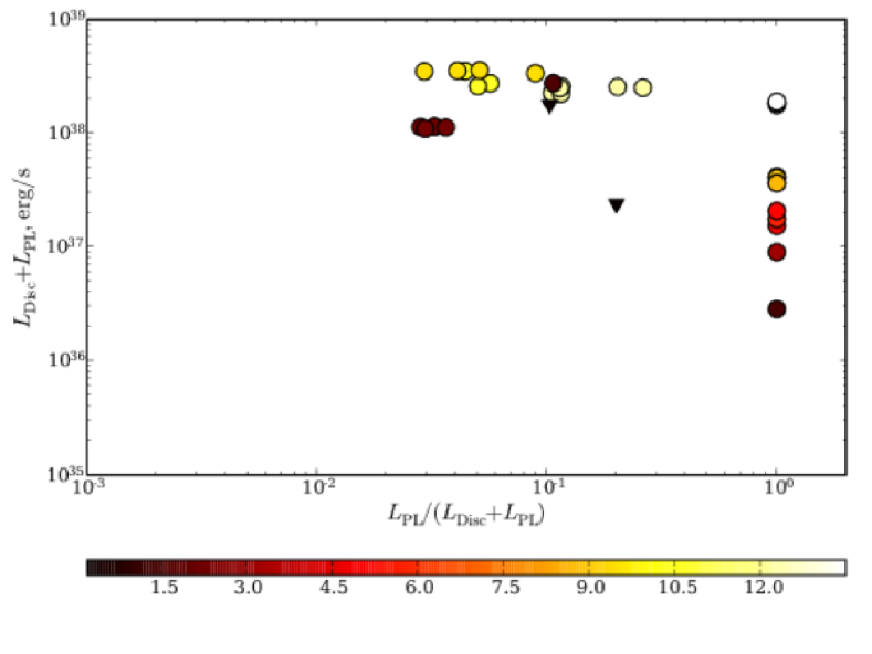
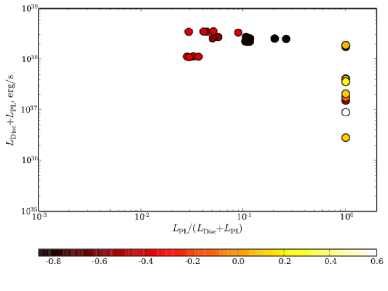
Figure 16: DFLD with left $8.5{\rm\thinspace GHz}$ radio flux in mJy and right $\alpha$ as the colour scale. Points which only have upper limits on the radio flux are shown by triangles.

As can be seen in Fig. 16, the highest radio fluxes are observed at the top of the DFLD. There is a sharp drop in radio flux as GX 339-4 drops to the bottom of the DFLD and heads back to the hard state. There is also a possibility that the radio flux decreases as GX 339-4 moves across the top of the DFLD.

In the right-hand panel of Fig. 16 the change of the radio spectrum between the hard and soft states is clear. The stalk of the DFLD has a spectral index of $\alpha\sim 0.2$, whereas the soft state has a spectral index of $\alpha\sim-0.4\to-0.6$.

9 Summary

We have performed a comprehensive and consistent investigation into the disc and iron lines detected in the X-ray emission from GX 339-4. All the 913 public observations in the 11 year RXTE archive were reduced, but only 634 had sufficient number of counts and flux to be analysed further. Three types of model were fitted to each observation; single powerlaw, broken powerlaw and a disc + powerlaw and the best fitting one chosen. The spectra were also tested for the presence of a Gaussian line at $6.4{\rm\thinspace keV}$. There were four outbursts in the data, but we concentrate on the two best sampled. The relative variation in flux and X-ray colour between these two outbursts are remarkably similar.

A significant iron line was detected in 400 of the 634 observations. There is an anti correlation between the flux and the equivalent width of the iron line for observations of the soft state (X-ray colour $<0.22$) of $EW\propto S_{3-10{\rm\thinspace keV}}^{-0.621}$. This is steeper than the range in slopes found in AGN. In the hard state the data are consistent with no correlation. As such there is an effect analogous to the X-ray Baldwin effect in AGN present in X-ray binaries in the soft state. We compare the powerlaw slope, the line equivalent width and X-ray colour of the spectra. The relation obtained is similar to that seen in a sample of AGN studied by Mattson et al. (2007). Therefore the behaviour of the line is hysteretical.

Theoretical arguments indicate that the decay in disc temperature with flux should mimic that for a black body, $S_{\rm Disc}\propto R^{2}T^{4}$. We find that the disc flux rather than the source flux needs to be used for this relation to be valid. In the soft state the decay in disc temperature matches the expected $S_{\rm Disc}\propto T^{4}$. The best fit, however, is steeper at $T^{4.75}$ resulting from the comparatively large scatter and small range in disc temperature. This implies that during the decay of the disc temperature in the soft state the inner radius of the disc is constant. Departures from a constant inner disc radius are non-physical, implying that the model for the emission is not appropriate or the spectral analysis is insufficiently detailed during the the intermediate states.

Following the method outlined in Körding et al. (2006) we construct a Disc Fraction Luminosity Diagram for GX 339-4. We find that the shape qualitatively matches that produced for AGN. Linking this with the radio emission from GX 339-4 the change in radio spectrum between the presence and absence of the disc is clearly visible. The large gap in the DFLD at low disc-high powerlaw fractions is surmised to result from the lack of spectral resolution at low energies. Summed spectra from different parts of the HID show that this is indeed the case for the low intermediate state.

10 Appendix: Spectral Fits

We show in Table 2 the results of fitting the models adopted for this analysis to the summed spectra. We only fit the models used in this analysis rather than more complex ones which would be appropriate for achieving a good fit to this high signal-to-noise data. We also show in Fig. 17 fits to the spectra which did not include a line component, as well as the fits used in Fig. 5 but with the line normalisation set to zero before producing the plot.

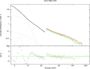
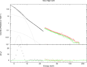
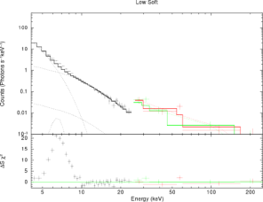
Figure 17: top: The disc + powerlaw models fitted to the data with no line component present. bottom:The disc + powerlaw + gaussian models fitted to the data, and then the normalisation of the line component set to zero before producing the plot.

Table 2:

References

- Baldwin (1977) Baldwin J. A., 1977, ApJ, 214, 679
- Belloni (2004) Belloni T., 2004, Nuclear Physics B Proceedings Supplements, 132, 337
- Belloni (2006) —, 2006, Advances in Space Research, 38, 2801
- Belloni et al. (2005) Belloni T., Homan J., Casella P., van der Klis M., Nespoli E., Lewin W. H. G., Miller J. M., Méndez M., 2005, A&A, 440, 207
- Belloni et al. (1997) Belloni T., Mendez M., King A. R., van der Klis M., van Paradijs J., 1997, ApJ, 479, L145+
- Belloni et al. (2000) Belloni T., Migliari S., Fender R. P., 2000, A&A, 358, L29
- Belloni et al. (2006) Belloni T., Parolin I., Del Santo M., Homan J., Casella P., Fender R. P., Lewin W. H. G., Méndez M., Miller J. M., van der Klis M., 2006, MNRAS, 367, 1113
- Bianchi et al. (2007) Bianchi S., Guainazzi M., Matt G., Fonseca Bonilla N., 2007, A&A, 467, L19
- Chaty et al. (2003) Chaty S., Haswell C. A., Malzac J., Hynes R. I., Shrader C. R., Cui W., 2003, MNRAS, 346, 689
- Corbel et al. (2000) Corbel S., Fender R. P., Tzioumis A. K., Nowak M., McIntyre V., Durouchoux P., Sood R., 2000, A&A, 359, 251
- Esin et al. (1997) Esin A. A., McClintock J. E., Narayan R., 1997, ApJ, 489, 865
- Falcke et al. (2004) Falcke H., Körding E., Markoff S., 2004, A&A, 414, 895
- Fender et al. (1999) Fender R., Corbel S., Tzioumis T., McIntyre V., Campbell-Wilson D., Nowak M., Sood R., Hunstead R., Harmon A., Durouchoux P., Heindl W., 1999, ApJ, 519, L165
- Fender et al. (2004) Fender R. P., Belloni T. M., Gallo E., 2004, MNRAS, 355, 1105
- Fender et al. (1997) Fender R. P., Spencer R. E., Newell S. J., Tzioumis A. K., 1997, MNRAS, 286, L29
- Gallo et al. (2004) Gallo E., Corbel S., Fender R. P., Maccarone T. J., Tzioumis A. K., 2004, MNRAS, 347, L52
- Gallo et al. (2003) Gallo E., Fender R. P., Pooley G. G., 2003, MNRAS, 344, 60
- George & Fabian (1991) George I. M., Fabian A. C., 1991, MNRAS, 249, 352
- Gierliński & Done (2004) Gierliński M., Done C., 2004, MNRAS, 347, 885
- Homan et al. (2001) Homan J., Wijnands R., van der Klis M., Belloni T., van Paradijs J., Klein-Wolt M., Fender R., Méndez M., 2001, ApJS, 132, 377
- Hynes et al. (2004) Hynes R. I., Steeghs D., Casares J., Charles P. A., O’Brien K., 2004, ApJ, 609, 317
- Iwasawa & Taniguchi (1993) Iwasawa K., Taniguchi Y., 1993, ApJ, 413, L15
- Kong et al. (2000) Kong A. K. H., Kuulkers E., Charles P. A., Homer L., 2000, MNRAS, 312, L49
- Körding et al. (2006) Körding E. G., Jester S., Fender R., 2006, MNRAS, 372, 1366
- Körding et al. (2007) Körding E. G., Migliari S., Fender R., Belloni T., Knigge C., McHardy I., 2007, MNRAS, 380, 301
- Maccarone (2003) Maccarone T. J., 2003, A&A, 409, 697
- Markert et al. (1973) Markert T. H., Canizares C. R., Clark G. W., Lewin W. H. G., Schnopper H. W., Sprott G. F., 1973, ApJ, 184, L67+
- Mattson et al. (2007) Mattson B. J., Weaver K. A., Reynolds C. S., 2007, ArXiv e-prints, 704
- McClintock et al. (2001) McClintock J. E., Haswell C. A., Garcia M. R., Drake J. J., Hynes R. I., Marshall H. L., Muno M. P., Chaty S., Garnavich P. M., Groot P. J., Lewin W. H. G., Mauche C. W., Miller J. M., Pooley G. G., Shrader C. R., Vrtilek S. D., 2001, ApJ, 555, 477
- McClintock & Remillard (2006) McClintock J. E., Remillard R. A., 2006, Black hole binaries, Compact stellar X-ray sources, pp. 157–213
- McClintock et al. (2007) McClintock J. E., Remillard R. A., Rupen M. P., Torres M. A. P., Steeghs D., Levine A. M., Orosz J. A., 2007, astro-ph/0705.1034, 705
- McHardy et al. (2006) McHardy I. M., Koerding E., Knigge C., Uttley P., Fender R. P., 2006, Nature, 444, 730
- Merloni et al. (2000) Merloni A., Fabian A. C., Ross R. R., 2000, MNRAS, 313, 193
- Merloni et al. (2003) Merloni A., Heinz S., di Matteo T., 2003, MNRAS, 345, 1057
- Miller et al. (2004a) Miller J. M., Fabian A. C., Reynolds C. S., Nowak M. A., Homan J., Freyberg M. J., Ehle M., Belloni T., Wijnands R., van der Klis M., Charles P. A., Lewin W. H. G., 2004a, ApJ, 606, L131
- Miller et al. (2006) Miller J. M., Homan J., Steeghs D., Rupen M., Hunstead R. W., Wijnands R., Charles P. A., Fabian A. C., 2006, ApJ, 653, 525
- Miller et al. (2004b) Miller J. M., Raymond J., Fabian A. C., Homan J., Nowak M. A., Wijnands R., van der Klis M., Belloni T., Tomsick J. A., Smith D. M., Charles P. A., Lewin W. H. G., 2004b, ApJ, 601, 450
- Miniutti et al. (2007) Miniutti G., Fabian A. C., Anabuki N., Crummy J., Fukazawa Y., Gallo L., Haba Y., Hayashida K., Holt S., Kunieda H., Larsson J., Markowitz A., et al, 2007, PASJ, 59, 315
- Miyamoto et al. (1995) Miyamoto S., Kitamoto S., Hayashida K., Egoshi W., 1995, ApJ, 442, L13
- Nandra et al. (1997) Nandra K., George I. M., Mushotzky R. F., Turner T. J., Yaqoob T., 1997, ApJ, 488, L91+
- Page et al. (2004) Page K. L., O’Brien P. T., Reeves J. N., Turner M. J. L., 2004, MNRAS, 347, 316
- Protassov et al. (2002) Protassov R., van Dyk D. A., Connors A., Kashyap V. L., Siemiginowska A., 2002, ApJ, 571, 545
- Reynolds & Nowak (2003) Reynolds C. S., Nowak M. A., 2003, Physics Reports, 377, 389
- Rossi et al. (2005) Rossi S., Homan J., Miller J. M., Belloni T., 2005, MNRAS, 360, 763
- Shahbaz et al. (2001) Shahbaz T., Fender R., Charles P. A., 2001, A&A, 376, L17
- Shimura & Takahara (1995) Shimura T., Takahara F., 1995, ApJ, 445, 780
- Stocke et al. (1992) Stocke J. T., Morris S. L., Weymann R. J., Foltz C. B., 1992, ApJ, 396, 487
- Sunyaev & Revnivtsev (2000) Sunyaev R., Revnivtsev M., 2000, A&A, 358, 617
- Terashima & Wilson (2003) Terashima Y., Wilson A. S., 2003, ApJ, 583, 145
- Tomsick et al. (2005) Tomsick J. A., Corbel S., Goldwurm A., Kaaret P., 2005, ApJ, 630, 413
- Ueda et al. (1994) Ueda Y., Ebisawa K., Done C., 1994, PASJ, 46, 107
- van der Klis (1995) van der Klis M., 1995, in X-ray Binaries, Lewin W. H., van Paradjis J., van den Heuvel E. P. J., eds., CUP, p. 252
- Wardziński et al. (2002) Wardziński G., Zdziarski A. A., Gierliński M., Eric Grove J., Jahoda K., Neil Johnson W., 2002, MNRAS, 337, 829
- Wilms et al. (1999) Wilms J., Nowak M. A., Dove J. B., Fender R. P., di Matteo T., 1999, ApJ, 522, 460
- Yu et al. (2007) Yu W., Lamb F. K., Fender R., van der Klis M., 2007, ApJ, 663, 1309
- Zdziarski et al. (2004) Zdziarski A. A., Gierliński M., Mikołajewska J., Wardziński G., Smith D. M., Alan Harmon B., Kitamoto S., 2004, MNRAS, 351, 791
- Zdziarski et al. (1998) Zdziarski A. A., Poutanen J., Mikolajewska J., Gierlinski M., Ebisawa K., Johnson W. N., 1998, MNRAS, 301, 435