Predictor-Corrector Preconditioners for Newton-Krylov Solvers in Fluid Problems

Abstract

We propose an alternative implementation of preconditioning techniques for the solution of non-linear problems. Within the framework of Newton-Krylov methods, preconditioning techniques are needed to improve the performance of the solvers. We propose a different implementation approach to re-utilize existing semi-implicit methods to precondition fully implicit non-linear schemes. We propose a predictor-corrector approach where the fully non-linear scheme is the corrector and the pre-existing semi-implicit scheme is the predictor. The advantage of the proposed approach is that it allows to retrofit existing codes, with only minor modifications, in particular avoiding the need to reformulate existing methods in terms of variations, as required instead by other approaches now currently used. To test the performance of the approach we consider a non-linear diffusion problem and the standard driven cavity problem for incompressible flows.

1 Introduction

A classic problem of computational science and engineering is the search for an efficient numerical scheme for solving non-linear time-dependent partial differential equations. Explicit and semi-implicit methods can provide simple solution techniques but are seriously limited by time step limitations for stability (explicit methods) and accuracy (semi-implicit methods).

Recently, significant progress has been made in the development of fully implicit approaches for solving nonlinear problems: the Newton-Krylov (NK) method [1, 2]. The method is developed from the Newton iterative method, by applying a linear iterative solver to the Jacobian equation for the Newton step and terminating that iteration when a suitable convergence criterion holds.

For the solution of the linear Jacobian equation, Krylov methods are often the choice, leading to the Newton-Krylov (NK) approach. However, for most cases, Krylov solvers can be extremely inefficient. The need for good preconditioners techniques becomes a constraining factor in the development of NK solvers [3].

In a number of fields, recent work based on multi-grid and physics-based preconditioners [4, 5, 6] have demonstrated extremely competitive performances.

In the present study, we present a different implementation of preconditioning: the predictor-corrector (PC) preconditioner. The approach has two novelties. First, it preconditions directly the non-linear equations rather than the linear Jacobian equation for the Newton step. The idea is not new [1], but it is implemented here in a new way that leads to great simplifications of the implementation. We note that this simplification is designed also to minimize the effort in refitting existing semi-implicit codes into full fledged implicit codes, representing perhaps a greater advance in software engineering than in computational science. Second, we test new ways of preconditioning the equations by using a combination of predictor-corrector semi-implicit preconditioning.

The fundamental idea is to use a predictor to advance a semi-implicit discretization of the governing equations and use a corrector Newton step to correct for the initial state of the predictor step. The typical NK solver is used to compute the unknown value of the state vector at the end of the time step ${\bf x}^{1}$ from its known value at the previous time step ${\bf x}^{0}$. Instead, we use the Newton method to iterate for a modification of the actual known state ${\bf x}^{*}$ from the previous time step to find a modified ”previous” state that makes the semi-implicit predictor step give the solution of the fully implicit method.

Two advantages are obvious. First, the actual previous state ${\bf x}^{0}$ is likely to be a better first guess for the modified initial state ${\bf x}^{*}$ of the predictor than it is for the final state of the corrector step. Second, by modifying the non-linear function and consequently modifying the Jacobian equation, the PC preconditioner modifies the spectral properties of the Jacobian matrix in the same way as preconditioners applied directly to the Jacobian equation. Indeed, as shown below the PC preconditioner gives the same type of speed-up of the Krylov convergence without requiring to formulate an actual preconditioning of the Krylov solver.

We use a non-lnear diffusion problem and the standard driven cavity flow problem as benchmarks to demonstrate the preformance and the reliability of the PC preconditioning method.

2 The Preconditioned Newton-Krylov Approach

Most discretization schemes can be expressed as a set of difference equations for a set of unknowns $\bf x$ representing the unknown fields on a spatial grid. Once the time is discretized, the state vector $\bf x$ is computed at a sequence of discrete time levels. We label the initial state of a time step (corresponding to the final time of the previous time step) as ${\bf x}^{0}$ and the final time as ${\bf x}^{1}$.

When the time discretization scheme is fully implicit, the most general two-level scheme can be formulated as a non-linear relationship between ${\bf x}^{0}$ and ${\bf x}^{1}$:

$$f({\bf x}^{0},{\bf x}^{1})=0$$ (1)

where the vector function $f$ depends both on the initial and the final states. The implicit nature of the scheme resides in the fact that the function $f$ is a function of the new time level, requiring the solution of a set of non-linear (if the function $f$ is non-linear) coupled equations. As noted above this can be accomplished with the NK method [1]. The method is based on solving the Jacobian equation obtained linearizing the difference eq. (1) around the current available estimate ${\bf x}_{k}^{1}$ of the solution in the Newton iteration:

$$f({\bf x}^{0},{\bf x}_{k}^{1})+J\delta{\bf x}=0$$ (2)

where $J=\partial f/\partial{\bf x}^{1}$ is the Jacobian matrix and $\delta{\bf x}$ is the correction leading to the new estimation by the Newton iteration: ${\bf x}_{k+1}^{1}={\bf x}_{k}^{1}+\delta{\bf x}$.

The solution of eq. (2) is conducted with a Krylov solver. The Jacobian matrix is approximated by a difference:

$$J\delta{\bf x}=\frac{f({\bf x}^{0},{\bf x}_{k}^{1}+\epsilon\delta{\bf x})-f({\bf x}^{0},{\bf x}_{k}^{1})}{\epsilon}$$ (3)

with $\epsilon$ chosen according to the machine precision [1]. Here we use the inexact Newton method [2], based on relaxing the convergence criterion on the solution of the Jacobian equation when the Newton equation is still far from convergence and progressively tightening it as the Newton iterations close in on the solution. The specific algorithm used here follows closely the implementation in the textbook by Kelley [1]. For the Krylov solver we use GMRES [7] since the Jacobian matrix can be non symmetric.

While the pure NK method works in giving a solution, the number of Krylov iterations required for each Newton step to solve eq. (2) can be staggering. In particular, as the grid is refined and the size of the unknown vector ${\bf x}^{1}$ is increased the number of Krylov iterations tends to increase. This is the reason why a preconditioner is needed.

A remarkable feature of the NK method is its ability to be regarded as a black box, communicating with the rest of the code only via the evaluation of the non-linear function that summarize the discretized partial differential equations. The NK black box provides as an output a succession of guesses for the solution ${\bf x}^{1}_{k}$ and requires as an input a residual coming from the function evaluation ${\bf r}_{k}$. At convergence, the residual is reduced to a prescribed tolerance:

$${\bf r}_{k}<\eta_{a}+\eta_{r}{\bf r}_{0}$$ (4)

where the absolute tolerance $\eta_{a}$ and the relative tolerance $\eta_{r}$ can be chosen by the user.

Most of the usual preconditioning techniques open the black box and fiddle with the Krylov solver by enveloping a preconditioner around the Krylov solver for the Jacobian equation to improve its performance. This is accomplished in a number of very successful methods that lead to nearly ideal performance [4]. The approach is perfectly suited to new codes that can easily be designed to implement the most effective preconditioners.

However, sometimes the need arises for retrofitting existing semi-implicit codes. The goal in that case, is to use the existing code as a preconditioner for a fully implicit approach. The new fully implicit approach provides the non-linear function evaluation for NK. The old code provides the preconditioner. In the usual approach, the black box of the NK need to be opened and the old code need to be modified to provide a representation for the Jacobian of the new fully implicit method. A major part of the modification is the fact that preconditioners act on Krylov vectors that are not physical quantities but rather their change from Newton iteration to Newton iteration as in eq. (2).

Pre-existing codes operate on full fields, with their boundary conditions, not on variations. The change to accommodate this need can be considerable. We propose here a way to formulate preconditioning techniques that does not require to operate on variations but can operate directly on the fields themselves and leaves the NK black box closed allowing the user to simply deploy existing NK tools.

To arrive at the method, we remind that preconditioning can be regarded in two ways. First, one can view preconditioning as a modification of the Krylov step only. We focus here on the so-called right preconditioning approach [1]. In that case, the Jacobian problem is reformulated as:

$$f({\bf x}^{0},{\bf x}_{k}^{1})+JP^{-1}P\delta{\bf x}=0$$ (5)

where the preconditioning matrix is chosen so that $JP^{-1}$ is an approximation to the identity matrix, as it is when $P$ approximates $J$. This point of view opens the NK black box and fiddles with the Jacobian equation.

The approach followed here is based on an alternative look at the preconditioning step presented in the classic textbook by Kelley [1]. The preconditioning step can be regarded as a modification of the non-linear function itself. The advantage of this second perspective is two-fold. First, the black box of NK need not be opened and the modifications required for preconditioning can be done directly on the non-linear function evaluation. Second, this point of view leads the way to an approach that acts directly on the full fields, and not on their variations. As mentioned above, this feature is key in retrofitting existing codes.

3 Predictor-Corrector Preconditioners

In the present study, a preconditioner is constructed by using the predictor-corrector method. The key idea lies on modifying the non linear function evaluation that provides the residual for the NK iteration.

The approach requires to design alongside the fully implicit scheme in eq. (1), a second semi-implicit method. We note that this is typically no hardship as semi-implicit methods were developed and widely used before the implicit methods became tractable. Using the same notation, we can write the most general two-level semi-implicit algorithm as:

$$A{\bf x}^{1}+f_{SI}({\bf x}^{0})=0$$ (6)

where $A$ is a linear operator (matrix) and the function $f_{SI}$ depends only on the old state ${\bf x}^{0}$. The semi-implicit nature of the scheme resides on the fact that the difference eq. (6) depends non-linearly on the (known) old state ${\bf x}^{0}$ but only linearly on the new (unknown) state ${\bf x}^{1}$.

In the classic implementation of preconditioners [4], the equation for the semi-implicit scheme (6) is rewritten in terms of the modification $\delta{\bf x}$ in a given Newton iteration:

$$A\delta{\bf x}={\bf r}_{k}$$ (7)

where ${\bf r}_{k}=f({\bf x}_{k}^{1},{\bf x}^{0})$ is the residual of the current Newton iteration. The matrix $A$ of the semi-implicit scheme becomes the preconditioner matrix $P$ for the Jacobian matrix $J$ of eq. (2). The approach has been extremely successful in terms of providing a robust and effective solution scheme. For example in the case of incompressible flows, the number of Krylov iteration has been shown [6, 5] to be reduced drastically and to become nearly independent of the grid size.

However, a substantial modification of existing codes follows from the need to modify the GMRES solver to use the matrix $A$ as a preconditioner, especially when the method is formulated in a matrix-free form where the matrix $J$ and the matrix $A$ are not explicitly computed and stored.

We propose a different approach. We consider the following predictor-corrector algorithm:

$$\left\{\begin{array}[]{l}\displaystyle({\rm P})\;A{\bf x}^{1}+f_{SI}({\bf x}^{*})=0\\ \displaystyle({\rm C})\;{\bf r}=f({\bf x}^{0},{\bf x}^{1})\end{array}\right.$$ (8)

The predictor step uses the semi-implicit scheme to predict the new state ${\bf x}^{1}$ starting from a modification of the initial state ${\bf x}^{*}$. The corrector step computes the residual ${\bf r}$ for the fully implicit scheme when ${\bf x}^{1}$ from the predictor step is used.

We propose to use scheme (8) by using ${\bf x}^{0}$ as the initial guess of ${\bf x}^{*}$ and using the NK method to find the solution for ${\bf x}^{*}$ that makes the residual ${\bf r}$ of the corrector equation vanish. Once ${\bf r}=0$ (within a set tolerance), the fully implicit scheme is solved, but it is solved not iterating directly for ${\bf x}^{1}$ but iterating for the ${\bf x}^{*}$ that makes the predictor step predict the correct solution ${\bf x}^{1}$ of the corrector step.

Two points are worth noting.

First, we have modified the task of the NK iteration changing our unknown variable from ${\bf x}^{1}$ to ${\bf x}^{*}$. This corresponds to change the non-linear residual function that the Newton method needs to solve. To analyze this point, we consider a first order Taylor series expansion of the preconditioned non-linear function:

$$f({\bf x}^{0},-A^{-1}f_{SI}({\bf x}^{*}_{k}+\delta{\bf x}^{*}))=f({\bf x}^{0},-A^{-1}f_{SI}({\bf x}^{*}_{k}))-\frac{\partial f}{\partial{\bf x}^{1}}A^{-1}\frac{\partial f_{SI}}{\partial{\bf x}^{*}}\delta{\bf x}^{*}$$ (9)

We observe that by first order Taylor expanding the preconditioner step a relationship can be determined between the change$\delta{\bf x}^{*}$ and the corresponding change in the end state $\delta{\bf x}$:

$$A{\bf x^{1}_{k}}+A\delta{\bf x}+f_{SI}({\bf x}^{*}_{k})+\frac{\partial f_{SI}}{\partial{\bf x}^{*}}\delta{\bf x}^{*}=0$$ (10)

Recalling that at the $k$-th iteration the preconditioner equation was satisfied, i.e. $A{\bf x^{1}_{k}}+f_{SI}({\bf x}^{*}_{k})=0$, it follows that

$$\frac{\partial f_{SI}}{\partial{\bf x}^{*}}\delta{\bf x^{*}}=-A\delta{\bf x}$$ (11)

Using eq.(11) and recalling the definition $J=\partial f/\partial{\bf x}^{1}$, we can formally rewrite the Jacobian equation for the preconditioned step:

$$JA^{-1}A\delta{\bf x}={\bf r}_{k}$$ (12)

The equivalence of our approach to preconditioning and the standard approach is now manifest. To first order in the Taylor series expansion, the new approach is identical to applying the traditional preconditioners directly to the Jacobian equation [1]. However, to higher order this might be a better approach as it reduces the distance between the initial guess (${\bf x}^{0}$) and the solution for ${\bf x}^{*}$. If the semi-implicit method works properly, ${\bf x}^{0}$ is closer to the converged ${\bf x}^{*}$ than to the final state ${\bf x}^{1}$.

Second, programming the PC preconditioner is easier. The NK solver can be used as a black box, without any need to formally go into it and modify the Jacobian eq. (2) by adding a preconditioner. The semi-implicit method can be used directly on the actual states and not on their variation $\delta{\bf x}$ between two subsequent Newton iterates. This latter operation is complex as boundary conditions and source terms in equations need to be treated differently.

The approach described above is ideally suited for refitting an existing semi-implicit code by simply taking an off the shelf NK solver and wrapping it around the semi-implicit method already implemented. The only change being that in the semi-implicit scheme the initial state ${\bf x}^{0}$ is replaced by the guess of ${\bf x}^{*}$ provided by the NK solver. We have indeed proceeded in this fashion by wrapping the standard NK solver provided in the classic textbook by Kelley [1] around our previously written semi-implicit solver for the examples considered below.

4 Numerical Experiments

To test the method developed above, we present below two classic benchmarks: time-dependent diffusion in presence of a non-linear diffusion coefficient and relaxation of an incompressible flow driven in a cavity.

4.1 Non-linear Diffusion

The non-linear diffusion equation in non dimensional units and in 1D cartesian geometry is:

$$\frac{\partial\phi}{\partial t}=\frac{\partial}{\partial x}\left(D(\phi)\frac{\partial\phi}{\partial x}\right)$$ (13)

where $\phi$ is the quantity being evolved. The diffusion coefficient is chosen as $D(\phi)=\alpha_{0}+\alpha_{1}\phi$ with $\alpha_{0}=\alpha_{1}/10$ and $\alpha_{1}=1$.

The initial condition is $\phi=x\sin(x/L)/L$ and the boundary conditions are $\phi(0)=0$ and $\phi(L)=0$ with $L=4$.

The method described above is implemented using a fully implicit Crank-Nicolson scheme for the corrector step and a semi-implicit scheme based on lagging the diffusion coefficient as predictor. In space, the second order operator is discretized with centered differencing.

The residual evaluation for the fully implicit (corrector) step is

$$r_{i}=\frac{\phi_{i}^{1}-\phi_{i}^{0}}{\Delta t}-\frac{D_{i+1/2}^{1/2}}{\Delta x^{2}}\left(\phi^{1/2}_{i+1}-\phi^{1/2}_{i}\right)+\frac{D_{i-1/2}^{1/2}}{\Delta x^{2}}\left(\phi^{1/2}_{i}-\phi^{1/2}_{i-1}\right)$$ (14)

where $\phi^{1/2}_{i}=(\phi^{1}_{i}+\phi^{0}_{i})/2$ and $D^{1/2}_{i+1/2}=D((\phi^{1/2}_{i+1}+\phi^{1/2}_{i})/2)$.

For the predictor step we use:

$$\frac{\phi_{i}^{1}-\phi_{i}^{*}}{\Delta t}=\frac{D_{i+1/2}^{0}}{\Delta x^{2}}\left(\phi^{1/2*}_{i+1}-\phi^{1/2*}_{i}\right)-\frac{D_{i-1/2}^{0}}{\Delta x^{2}}\left(\phi^{1/2*}_{i}-\phi^{1/2*}_{i-1}\right)$$ (15)

where $\phi^{1/2*}_{i}=(\phi^{1}_{i}+\phi^{*}_{i})/2$ and the diffusion coefficient is lagged using the actual value of the old time level $\phi^{0}$. As prescribed in the method described above, the predictor is modified by introducing the fictitious initial value $\phi^{*}_{i}$ that is the actual unknown solved for by the NK method.

The procedure is as follows:

1. The NK method provides the guess of $\phi^{*}_{i}$ (the initial guess being the old state $\phi^{0}$).

2. The predictor equation 15 is solved (using a simple tridiagonal solver) for the advanced value of the unknown $\phi^{1}_{i}$

3. The residual of the corrector equation 14 is computed and fed back to the NK solver to compute the new guess of $\phi^{*}_{i}$.

To solve the non-linear system we developed a program that used the NK solver downloaded by the web site relative to the textbook by Kelley [1]. For the convergence test, eq. (4), we used $\eta_{r}=10^{-5}$, $\eta_{a}=10^{-5}$ and we deployed the Eisenstat-Walker inexact convergence criterion for the solution of the Jacobian equation [8]. The Krylov solver used is GMRES [7].

The problem does not have an analytical solution and we report for reference the initial and final states (at $t=1.0$) in the most refined simulation considered (800 cells), Fig. 1.

Figure 1: Fiducial solution (obtained on a 800 cells grid) for the non linear diffusion problem. The initial state is the dotted line, the final state (t=1) is the solid line.

We have compared the efficiency of the NK solver with and without the PC preconditioner described above. We change the number of cells but hold the time step at $\Delta t=10^{-1}$, continuing the simulation until the final time $t=1.0$. Table. 1 reports the number of Newton and Krylov iterations for different grid sizes. Three trends emerge clearly. First, the number of Krylov iterations is reduced drastically by the proconditioner in all cases, even on the coarsest grid. Second, the number of Krylov iterations in the unpreconditioned case scales in a very unfavorable way with the number of cells increasing as the grid is refined, compounding the increased cost of each iterations. Instead, with the preconditioner the number of iterations remain essentially constant on all grids, resulting in a virtually ideal scaling. Finally, even with the present tests conducted with a straight-forward non-optimized code, the actual CPU time of the preconditioned runs is always smaller, resulting in a factor of 7 saving in the most refined grid. We point out that this is rather remarkable in a simple 1D test. The savings to be expected in 2D would be compounded by the dimensionality.

Table 1: Number of Newton and Krylov (GMRES) iterations and CPU time (in seconds) for different uniform grids, with and without preconditining. Tests conducted on a Windows XP operating system with 1GB ram memory and Pentium M 1.4GHz.

Grid	Preconditioned			Un-Preconditioned
N	Newton	Krylov	CPU Time	Newton	Krylov	CPU Time
100	2.82	3.18	0.19	3.09	15.74	0.32
200	3.00	3.64	0.28	3.09	29.21	0.67
400	3.00	3.82	0.43	3.09	53.80	1.75
800	3.00	4.67	0.93	3.82	109.40	6.42

4.2 Driven Cavity Flow

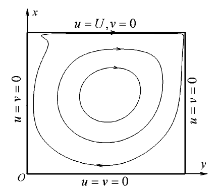
Figure 2: Standard driven cavity flow and the velocity boundary conditions

Next we consider the standard driven 2-D incompressible cavity flow [9]. The geometry and the velocity boundary conditions are shown in Fig. 2. The following non-dimensional variables are introduced:

$$(u,v)=\frac{(\hat{u},\hat{v})}{U}\,,\;(x,y)=\frac{(\hat{x},\hat{y})}{L}$$ (16)

where the hatted variables represent the dimensional variables. The scales are the cavity width $L$ and the upper boundary velocity $U$. Time is normalized accordingly. The governing equation, in term of the vorticity $\omega$, and the stream function $\psi$, can be expressed as:

$$\frac{\partial^{2}\psi}{\partial x^{2}}+\frac{\partial^{2}\psi}{\partial y^{2}}=-\omega$$ (17)

$$\frac{\partial\omega}{\partial t}+u\frac{\partial\omega}{\partial x}+v\frac{\partial\omega}{\partial y}=\frac{1}{{\rm Re}}\left(\frac{\partial^{2}\omega}{\partial x^{2}}+\frac{\partial^{2}\omega}{\partial y^{2}}\right)$$ (18)

where $u=\partial\psi/\partial y$, $v=-\partial\psi/\partial x$, $\omega=\partial v/\partial x-\partial u/\partial y$ , and ${\rm Re}=UL/\nu$ is the Reynolds number based on the viscosity $\nu$. Dirichlet boundary conditions are applied for the stream function and the boundary conditions for vorticity is determined by the physical boundary conditions on the velocity [10]. For example, at the left wall $\omega=\partial v/\partial x=-\partial^{2}\psi/\partial y^{2}$. We can obtain expressions for $\omega$ at other walls in an analogous manner.

Eqs. (17) and (18) are discretized using the centered difference scheme in space. Two types of discretization are considered in time, the semi-implicit Euler scheme (where the velocity in eq.(18) is taken at the initial time level of the time step) and the fully implicit Euler scheme.

We test the PC preconditioner approach using a fully implicit backward Euler scheme for corrector:

$$r_{ij}=\frac{\omega^{1}_{ij}-\omega^{0}_{ij}}{\Delta t}+{\bf u}^{1}_{ij}\cdot{\mathbf{\Gamma}}_{ij}(\omega^{1})-\frac{1}{\rm Re}\Delta_{ij}(\omega^{1})$$ (19)

where the discretized gradient (Laplacian) operator is indicated as ${\mathbf{\Gamma}}_{ij}(\omega^{1})$ ($\Delta_{ij}(\omega^{1})$) and is evaluated using the new state $\omega^{1}$ in a fully implicit form. The velocity is computed also from the new state using the stream function elliptic equations in discretized form:

$$\Delta_{ij}(\psi^{1})=-\omega^{1}_{ij}$$ (20)

For preconditioning we use a semi-implicit scheme linearized by computing the velocity using the previous Newton iteration

$$\frac{\omega^{1}_{ij}-\omega^{*}_{ij}}{\Delta t}+{\bf u}^{1(k)}_{ij}\cdot{\mathbf{\Gamma}}_{ij}(\omega^{1})-\frac{1}{\rm Re}\Delta_{ij}(\omega^{1})$$ (21)

where the velocity is computed as:

$$\Delta_{ij}(\psi^{1}_{k})=-\omega^{1(k)}_{ij}$$ (22)

using the known vorticity from the previous Newton iteration. We remark that using the old velocity rather than the previous guess from the Newton iteration results in much poorer performances.

The code for the present test has been developed in Java using the prescriptions of the textbook by Kelley [1] as reference. The details of the implementation are identical as in the text above. We remark incidentally that Java is a suitable scientific computing language providing in its latest releases a competitive computing performance when compared with C++, C or even Fortran [11]. The resulting method is completely matrix-free as only matrix-vector products, rather than details of the matrix itself are needed. This circumstance greatly simplifies the application of the method to complex problems.

For reference, we present results for a case with a mesh of 129$\times$129 cells. The classic cavity flow solution is computed starting from a stagnant flow, allowing the boundary conditions to drive the cavity to a steady state. The flow condition at steady state is shown in Fig. 18. The figure is generated using the same contour lines used in the reference benchmark solution presented by Chia et al. [9]. We compared our solution with the published reference benchmark obtaining complete agreement.

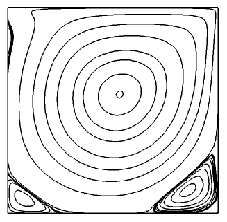
Figure 3: (a) Contours of stream function, (b) Contours of vorticity. Flow structure at steady state for Re=1000

We have compared the efficiency of the NK solver with and without the PC preconditioner described above. For the case without preconditioner, the number of Newton and GMRES iterations is reported in Table 2. In the preconditioned case, GMRES is never actually called thanks to the nearly perfect performance of the preconditioner that removes the need for multiple GMRES iterations. Table 2 reports the number of Newton iteration, corresponding also to the number of calls to the preconditioner, for this case. Total CPU times for the preconditioned and unpreconditioned case is also reported.

As one can readily see, the number of GMRES iterations increases without bounds in the unpreconditioned case, resulting in a corresponding unbounded increase in computational costs. In the last case in the table, the implicit case did not converge within the maximum allotted number of iterations allowed.

In contrast, the preconditioned case, requiring only 1 iteration of the preconditioner per Newton iterations, keeps the cost under control and converging in all cases considered. In the most refined cases, the gain exceed ten-fold, not mentioning the case where the unpreconditioned run failed.

Table 2: Number of Krylov (GMRES) iterations, calls of preconditioner and CPU time (in seconds) for different uniform grids and time step, of the fully implicit case and preconditioned semi-implicit cases. Tests conducted on a Windows XP operating system with 1GB ram memory and Pentium M 1.4GHz.

Grid	time step	Unpreconditioned			Preconditioned
N	$\Delta t$	Newton	Krylov	CPU Time	Newton	CPU Time
10	0.01	1.01	79.2	4	2.00	1
10	0.05	1.70	191.2	11	3.01	2
10	0.1	2.00	239.6	15	3.37	3
20	0.01	2.00	159.6	68	3.00	11
20	0.05	2.01	275.2	120	3.81	20
20	0.1	2.01	339.6	135	4.19	37
40	0.01	2.00	235.2	829	3.03	79
40	0.05	2.03	849.6	3122	4.28	308
40	0.1	2.26	2732.4	9667	4.96	661
60	0.01	2.01	287.6	2962	3.24	192
60	0.05	2.23	1798.8	15465	4.73	1042
60	0.1	–	–	–	5.31	1811

5 Conclusions

We presented a new implementation for preconditioning techniques based on using semi-implicit schemes to precondition fully implicit schemes. The fundamental new idea is to use the semi-implicit scheme as predictor and the fully implicit scheme as corrector, iterating the NK method on a modification of the old state used as initial state for the predictor rather than iterating on the final state of the corrector step as is typically done.

There is one primary advantage to the new implementation. Simplicity. The approach has been developed specifically with the goal in mind of reusing off-the-shelf existing semi-implicit methods and codes without requiring any modifications. In particular, the new implementation does not require to formulate the preconditioning step in terms of changes from a reference step (the previous Newton iteration). This latter requirement of previous approaches typically requires to make substantial modifications to existing code and n particular to boundary conditions. This requirement is completely eliminated, we require only one change: the initial state for the value of the state variables at each time step is no longer given by the old state but by the NK iteration.

Most researchers and institutions have invested human efforts and capital in developing extremely sophisticated semi-implicit codes. Our approach allows to reutilize the invested effort without virtually any modification. An existing semi-implicit code can be built upon by supplying a new non-linear function evaluation for the new fully implicit scheme and a NK solver. Off-the-shelf NK solvers are available easily from freely available libraries such as TRILINOS [12] or PETSc [13] or can be easily implemented following the recipes of excellent textbooks [1] (the latter is the approach we followed).

References

References

- [1] C. T. Kelley. Iterative methods for linear and nonlinear equations. SIAM, Philadelphia, 1995.
- [2] P. N. Brown and Y. Saad. Hybrid Krylov methods for nonlinear systems of equations. SIAM J. Sci. Stat. Comput., 11:450–481, 1990.
- [3] Y. Saad. Iterative Methods for Sparse Linear Systems. PWS Publishing Company, Boston, 1996.
- [4] D. A. Knoll and D.E. Keyes. Jacobian-free Newton-Krylov methods: a survey of approaches and applications. J. Comput. Phys., 193:357–397, 2004.
- [5] D. A. Knoll and V.A. Mousseau. On Newton-Krylov multigrid methods for the incompressible Navier-Stokes equations. J. Comput. Phys., 163:262–267, 2000.
- [6] M. Pernice and M.D. Tocci. A Multigrid-Preconditioned Newton-Krylov method for the incompressible Navier-Stokes equations. SIAM J. Sci. Comput., 23:398–418, 2001.
- [7] Y. Saad and M.H. Schultz. GMRES: A generalized minimal residual algorithm for solving non-symetric linear systems. SIAM J. Sci. Stat. Comput., 7:856–869, 1986.
- [8] S.C Eisenstat and H.F. Walker. Globally convergent inexact Newton methods. SIAM J. Optim., 4:393, 1994.
- [9] U. Chia, K.N. Chia, and T. Shin. High-Re solutions for incompressible flow using the Navier-Stokes equations and a multigrid method. SIAM J. Sci. Comput., 23:398–418, 2001.
- [10] P.J. Roache. Fundamentals of Computational Fluid Dynamics. Hermosa Publ., Albuquerque, 1998.
- [11] S. Markidis, G. Lapenta, W.B. VanderHeyden, and Z. Budimlic̀. Implementation and performance of a Particle In Cell code written in Java. Concurrency Comput. Pract. Exper., 17:821, 2005.
- [12] Michael Heroux, Roscoe Bartlett, Vicki Howle Robert Hoekstra, Jonathan Hu, Tamara Kolda, Richard Lehoucq, Kevin Long, Roger Pawlowski, Eric Phipps, Andrew Salinger, Heidi Thornquist, Ray Tuminaro, James Willenbring, and Alan Williams. An Overview of Trilinos. Technical Report SAND2003-2927, Sandia National Laboratories, 2003.
- [13] S. Balay, W.D. Gropp, L. C. McInnes, and B. F. Smith. PETSc users manual. Technical Report ANL-95/11 - Revision 2.1.0, Argonne National Laboratory, 2001.