q-bio/yymmnnn

Thermodynamics of a model

for RNA folding

Matías G. dell’Erba

Departamento de Física, Facultad de Ciencias Exactas y Naturales, Universidad Nacional de Mar del Plata, Funes 3350, (7600), Mar del Plata, Argentina

Guillermo R. Zemba

Facultad de Ciencias Fisicomatemáticas e Ingeniería, Universidad Católica Argentina, Av. A. Moreau de Justo 1500, Buenos Aires, Argentina

and

Departamento de Fısica, C.N.E.A. Av.Libertador 8250, (1429) Buenos Aires, Argentina

We analyze the thermodynamic properties of a simplified model for folded RNA molecules recently studied by G. Vernizzi, H. Orland, A. Zee (in Phys. Rev. Lett. 94 (2005) 168103). The model consists of a chain of one-flavor base molecules with a flexible backbone and all possible pairing interactions equally allowed. The spatial pseudoknot structure of the model can be efficiently studied by introducing a $N\times N$ hermitian random matrix model at each chain site, and associating Feynman diagrams of these models to spatial configurations of the molecules. We obtain an exact expression for the topological expansion of the partition function of the system. We calculate exact and asymptotic expressions for the free energy, specific heat, entanglement and chemical potential and study their behavior as a function of temperature. Our results are consistent with the interpretation of $1/N$ as being a measure of the concentration of $\rm{Mg}^{++}$ in solution.

PACS numbers: 87.14gn , 02.10.Yn , 87.15.Cc

The applications of mathematical and statistical mechanics techniques to study suitable biological problems has been a successful area of recent research interest [1, 2, 3]. In particular, the study of the spatial and topological (pseudoknot) structure of DNA and RNA molecules is a successful example of the above [4, 5, 6, 7, 8, 9, 10, 11]. A RNA molecule is a heteropolymer strand made up of four types of nucleotides: uracil ($U$), adenine ($A$), guanine ($G$), and cytosine ($C$). The sequence of these bases from the $5^{\prime}$ to the $3^{\prime}$ end defines the primary structure of the molecule. In solution, at room temperature, different bases can pair with each other by means of saturating hydrogen bonds to give the molecule a stable shape in three dimensions, with $U$ bonding to $A$, $C$ to $G$, and wobble pair $G$ to $U$, all with different interaction energies. This last interaction (non Watson-Crick base pair) together with triplets, quartets, etc. has a important role in fold of the RNA molecule [12, 14, 13, 15]. The effect of stacking interactions also contributes to the stability of the molecule, making sets of adjacent bonds twist into the familiar Watson-Crick helices. Among all possible structures that arise from interaction between the bases, one defines the secondary structures of a RNA molecule as all structures which are represented by planar arc diagrams, that is, no crossing of arcs in a representation resembling a Feynman diagram. When the diagrams are non-planar, one says that a RNA molecule contains one or more pseudoknots (see [16, 17] for a general definition and [21] for a discussion on the planarity of the diagrams). Finally, one defines the tertiary structure of RNA as the actual spatial three-dimensional arrangement of the base sequence.

Several methods have been successfully used to study the folding dynamics of RNA molecules in various conditions. Some of these are based on statistical mechanics models, which usually avoid the complexities related to the dynamical evolution of the real world molecules, but allowing for a simple, kinematical treatment of the proposed models. Therefore, the study of these models can shed light on the intricate molecular dynamics and is our main motivation for considering them. In this paper, we study a simplified model of a RNA-like molecule considered in [5] in which the geometric degrees of freedom of the system, such as the stiffness and the sterical constraints of the chain, are not taken into account. In addition, they consider that all pairs of bases interact with a common pairing strength (the assumption of neglecting disorder along the sequence is actually a classic approximation [22]). Moreover, the model keeps the fundamental property of saturation of the interactions, that is, given a base in the chain it can interact (following the rules mentioned above) with only one another base at a time. The study of this model is interesting in itself and has motivated some interesting work in the literature, including case of the planar diagram limit (no pseudo-knots) [18][19][20], and the study of the tertiary structure of the RNA molecule (see, for instance [5, 6, 7, 8, 9]). Moreover, the model allows for some exact calculations including the partition function, the specific heat, and some other thermodynamical and physical quantities.Therefore, the study of the physical properties of this model could be considered as a first approximation or a limit case for more realistic RNA models. A natural extension of the model in [5] towards more realistic ones (for example, including different interactions between the bases) could be developed by simple modifications of a matrix potential.

The authors of [5] consider a system of $L$ molecules (nucleotide bases) forming a lineal macromolecule with the shape of a chain. They do not describe the formation of the backbone, but only the interaction between links of the chain that produce the folding of the RNA macromolecule (see Fig.1). Each base can interact through an attractive force with any other base of the chain. However, once a given molecule has paired with other, it will not interact again with another. In this case, it is said that the interaction between these bases saturate.

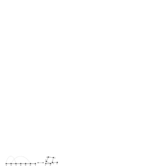
Figure 1: Arc diagram representation of the interacting pairs $(1,3)$ and $(2,6)$ and its respective folded diagram.

Although the bases that form the RNA molecule interact with different pairwise energies, a first simple approximation is to consider that this energy is the same for all bonds, and that any paring of bases is assumed to be feasible. This amounts to considering just one type of base and no further selection rules. Note that if all energies are equal, then the Boltzmann factors $v=e^{-\frac{\epsilon}{\kappa T}}$ (where $T$ is the absolute temperature and $\kappa$ is the Boltzmann constant which we will equal to one) are equal as well. The configurational partition function of a molecule of size $L$ in the model in [5] can be written as

$$Z(L,N,T)=\frac{1}{N}\langle{\rm tr}(1+\frac{1}{L^{1/2}}\varphi)^{L}\rangle=\frac{\int d\varphi\ e^{-\frac{N}{2Lv}{\rm tr}\varphi^{2}}\frac{1}{N}{\rm tr}(1+\frac{1}{L^{1/2}}\varphi)^{L}}{\int d\varphi\ e^{-\frac{N}{2Lv}{\rm tr}\varphi^{2}}},$$ (1)

where $\varphi$ is a random $N\times N$ hermitian matrix and $Z$ depend of $T$ through $v$. Note that the simple form of (1) is only a consequence of the symmetry of the matrix potential that reduces the original integration over $L$ matrices to one integration over $\varphi$ [5]. From the theory of random matrices (see for example [26], pag. 140-2) it follows that

$$\langle{\rm tr}\varphi^{2k}\rangle=\frac{(2k)!}{k!}\left(\frac{Lv}{2N}\right)^{k}\sum_{j=0}^{k}\left(\begin{array}[]{c}k\\ j\\ \end{array}\right)\left(\begin{array}[]{c}N\\ j+1\\ \end{array}\right)2^{j}\ ,$$ (2)

where all averages are performed with respect to the gaussian measure $d\varphi\ e^{-\frac{N}{2Lv}{\rm tr}\varphi^{2}}$. Replacing this into (1) and taking into account that $\langle{\rm tr}\varphi^{k}\rangle=0$ for $k$ odd, we arrive at:

$$Z(L,N,T)=\sum_{k=0}^{[L/2]}\sum_{j=0}^{k}\left(\begin{array}[]{c}L\\ 2k\\ \end{array}\right)\left(\begin{array}[]{c}k\\ j\\ \end{array}\right)\left(\begin{array}[]{c}N\\ j+1\\ \end{array}\right)\frac{(2k)!}{2^{k-j}\ k!\ N^{k+1}}\ v^{k}$$ (3)

where the symbol $[L/2]$ means the integer part of $L/2$. From (3) we may compute (for each $L$) $Z$ exactly, as a function of $N$ and $T$. The large-$N$ asymptotic expansion of $Z$ has a well-known topological meaning [31]: the power of $v$ is the number of arcs in the diagram, and the power of $1/N^{2}$ is the genus $g$ of the diagram. It is therefore convenient to write (3) in following form:

$$Z(L,N,T)=\sum_{k=0}^{[L/2]}d_{k}(L,N)\ e^{-\epsilon_{k}/T}$$ (4)

where $\epsilon_{k}=k\epsilon$ and

$$d_{k}(L,N)=\sum_{j=0}^{k}\left(\begin{array}[]{c}L\\ 2k\\ \end{array}\right)\left(\begin{array}[]{c}k\\ j\\ \end{array}\right)\left(\begin{array}[]{c}N\\ j+1\\ \end{array}\right)\frac{(2k)!}{2^{k-j}\ k!\ N^{k+1}}$$ (5)

From (4) we see that the spectrum of the system has $[L/2]+1$ possible energies $0,\epsilon,2\epsilon,\ldots,[L/2]\epsilon$ and the degeneracy of the $k-th$ level is $d_{k}(L,1)$. For example, for $L=7$ the maximum energy of a configuration is $3\epsilon$ and there are $d_{3}(7,1)=105$ different configurations with that energy. Moreover, considering (5) as a function of $N$ yields its topological information, e.g., for $L=7$, $d_{3}(7,N)=35+70\ 1/N^{2}$, which means that out of the total $105$ configurations with $3\epsilon$, $35$ have genus $0$ and $70$ have genus $1$.

Next, we calculate the partition function in the large $N$ limit, which is the planar limit, using the results of [24]. For completeness, we quote here the results relevant for ours. We define the resolvent $W(p)$:

$$W(p)=\frac{1}{N}\left\langle{\rm tr}\left(\frac{1}{p-\varphi}\right)\right\rangle=\sum_{n=0}^{\infty}\left(\frac{1}{p}\right)^{n+1}W_{n}\ ,$$ (6)

where $p$ is a complex variable, and

$$W_{n}=\frac{1}{N}\langle{\rm tr}\varphi^{n}\rangle\ .$$ (7)

In the large $N$ limit, the resolvent is given by the solution to the following equation called Pastur’s equation [25] (in the limit $g\rightarrow 0$ and $c\rightarrow 0$, in [24]):

$$W^{2}(p)-p\hskip 2.84544ptW(p)+1=0\ ,$$ (8)

which is:

$$W(p)=\sum_{k=0}^{\infty}C_{k}\frac{1}{p^{2k+1}}=\sum_{k=0}^{\infty}\frac{\left(\begin{array}[]{c}2k\\ k\\ \end{array}\right)}{k+1}\frac{1}{p^{2k+1}}\ ,$$ (9)

where $C_{k}$ are the Catalan numbers [27]. From (9) we obtain

$$\langle{\rm tr}\varphi^{2k}\rangle=\frac{\left(\begin{array}[]{c}2k\\ k\\ \end{array}\right)}{k+1}L^{k}v^{k}$$ (10)

With (10) we write down the partition function in the large $N$ limit. We consider the case $N=1$ for comparison purposes as well:

$$Z(L,N\rightarrow\infty,T)=\sum_{k=0}^{[L/2]}\frac{L!}{(L-2k)!\ k!\ (k+1)!}\ v^{k}$$ (11)

$$Z(L,N=1,T)=\sum_{k=0}^{[L/2]}\frac{L!}{(L-2k)!\ k!\ 2^{k}}\ v^{k}$$ (12)

Note that both expressions for $Z$ are very similar, except for the factors $(k+1)!$ and $2^{k}$ in the denominators of the expansion coefficients. Noting that the first factor is larger than the second, we conclude that $Z(N\rightarrow\infty)\leq Z(N=1)$. The interpretation of this result is clear if we recall that, for $v=1$, $Z(N\rightarrow\infty)$ counts the planar diagrams only, whereas $Z(N=1)$ counts both the planar and non-planar diagrams [5, 6, 7, 8]. Morevover, we verify that both partitions functions coincide for values of $L$ smaller than $3$ as they should given that all diagrams are planar in these cases. Furthermore, in these two limiting cases, the partition function can be written as in terms of hypergeometric functions:

$$Z(L,N=1,T)={{}_{2}F_{0}}(-\frac{L}{2},-\frac{L}{2}+\frac{1}{2};2v)\ ,$$ (13)

$$Z(L,N\rightarrow\infty,T)={{}_{2}F_{1}}(-\frac{L}{2},-\frac{L}{2}+\frac{1}{2};2;4v)\ ,$$ (14)

where ${{}_{p}F_{q}}(\overrightarrow{a};\overrightarrow{c};z)=\sum_{k=0}^{\infty}\frac{(a_{1})_{k}\ldots(a_{p})_{k}}{(c_{1})_{k}\ldots(c_{q})_{k}}\frac{z^{k}}{k!}$ and $(a)_{k}=\frac{\Gamma(a+k)}{\Gamma(a)}$ are the $k$-order Pochhammer symbols. We remark here that the results (13) and (14) are exact.

As we mentioned before, the power of $1/N^{2}$ yields the genus $g$ of the diagram, that is, the minimum number of handles of the surface on which the diagram can be drawn without crossings. From table of values of $Z$ for the smallest values of $L$ in [5] we notice, for instance, that for $L=5$ the number of planar diagrams on the sphere is $21$ and the number of non-planar diagrams that can be drawn on a torus without crossings is $5$. Next, we would like to write $Z(L,N,T)$ in the form of a topological expansion [31, 5, 6], that is, as a power series in the variable $1/N^{2}$:

$$Z(L,N,T)=\sum_{g=0}^{\infty}z_{g}(L,T)\frac{1}{N^{2g}}\ ,$$ (15)

where $z_{g}(L,\infty)$ is, for a molecule of size $L$, the number of planar diagrams in a topological surface of genus $g$. For the example of the previous paragraph, we have $z_{0}(5,\infty)=21$ and $z_{1}(5,\infty)=5$. Note that $z_{g}(L,T)$, as a function of $T$, is the partition function of the system living on the topological surface of genus $g$. In order to bring the partition function to the form (15), we first define the auxiliary function:

$$G_{k}(N)=\sum_{j=0}^{k}\left(\begin{array}[]{c}k\\ j\\ \end{array}\right)\left(\begin{array}[]{c}N\\ j+1\\ \end{array}\right)\frac{2^{j}}{N^{k+1}}.$$ (16)

This function contains all the $N$ dependence of (3). Below, we write the binomial coefficient as

$$\left(\begin{array}[]{c}N\\ j+1\\ \end{array}\right)=\frac{1}{(j+1)!}N(N-1)\cdots(N-j)=\frac{1}{(j+1)!}\sum_{m=0}^{j+1}S_{j+1}^{(m)}N^{m}\ ,$$ (17)

where $S_{j}^{(m)}$ is the Stirling number of the first kind [27, 28] with parameters $m,j$ (in turn, we define $S_{j}^{(m)}=0$ if $m>j$ or if $j\leq 0$). Replacing (17) in (16), we obtain

$$G_{k}(N)=\sum_{j=0}^{k}\left(\begin{array}[]{c}k\\ j\\ \end{array}\right)\frac{2^{j}}{(j+1)!}\sum_{m=0}^{j+1}\frac{S_{j+1}^{(m)}}{N^{k+1-m}},$$ (18)

Now, if we want to obtain the $O(1/N^{2g})$ of $G_{k}(N)$ (we indicate this by $G_{k}^{(2g)}(N)$), we must require that $k+1-m=2g$, then $j=k-2g,k-2g+1,\ldots,k$. To obtain all orders of $N$ we must add all possible values of $g$:

$$G_{k}(N)=\sum_{g=0}^{\infty}G_{k}^{(2g)}(N)=\sum_{g=0}^{\infty}\sum_{j=k-2g}^{k}\left(\begin{array}[]{c}k\\ j\\ \end{array}\right)\frac{2^{j}}{(j+1)!}\frac{S_{j+1}^{(k+1-2g)}}{N^{2g}},$$ (19)

replacing in (3) we obtain (15) with $z_{g}(L,T)$ given by:

$$z_{g}(L,T)=\sum_{k=0}^{[L/2]}\sum_{j=k-2g}^{k}\frac{L!\ 2^{j-k}\ S_{j+1}^{(k+1-2g)}}{(L-2k)!\ (k-j)!\ j!\ (j+1)!}\ e^{-\epsilon_{k}/T}.$$ (20)

In the limit $T\rightarrow\infty$, $z_{g}(L,T)$ coincides with $a_{L,g}$ of [5]. Using the above mentioned property of the Stirling numbers, we see from (20) that the maximum genus of a diagram for a given $L$ is $[L/4]$, therefore $g\leq[L/4]$. An analysis of the $T$-dependent phase transition from the topological expansion of the partition function will be given in a future publication [32].

In the rest of this letter, we analyze the thermodynamic properties implied by the partition functions (3) by studying some interesting observables. We start by considering the ’entanglement’ (non-local two-point correlation function) between two bases of the the chain in our model. For that, we use the following definition for the correlation between the molecules $i$ and $j$ ($i<j$) of the chain of size $L$

$$\langle i,j\rangle=\frac{Z(\overline{j-i},N,T)}{Z(L,N,T)},$$ (21)

where $Z(\overline{j-i},N,T)$ is the partition function for the molecule including bases $i$ up to $j$. For the case of periodic boundary conditions we have $Z(\overline{j-i},N,T)=Z(j-i+1,N,T)$. In the low temperature limit the partition function becomes independent of $N$ (in this limit only configurations up to two bases interacting are possible, it is, planar configurations). Therefore yields the same result for both the $N=1$ and $N\rightarrow\infty$ cases:

$$\langle i,j\rangle=\frac{1+\frac{1}{2}x(x+1)v}{1+\frac{1}{2}L(L-1)v}\simeq 1-\frac{1}{2}(L^{2}-x^{2})e^{-\beta\epsilon}\ ,$$ (22)

with $L>>1$, $x=j-i>>1$ (provided $\beta\epsilon>>\ln(L^{2}/12)+\ln(2+1/N^{2})$). The physical behavior of this observable can be obtained by considering the situation where $x$ is large, yielding $\langle i,j\rangle\simeq x^{2}$, which can be interpreted as a signal of confinement (long-range order with critical exponent $-2$). This behavior is coherent with the interpretation of the model as describing a folded RNA molecule. Note that the exponent $(-2)$ for the long range order coincides with the value found in [20, 23].

Going ahead with our study of observables of the model, we now calculate the normalized free energy $f$, or free energy per molecule, in the limit of low temperature:

$$f(L,N,T)=\frac{F(L,N,T)}{L}=-\frac{1}{\beta L}\ln(Z(L,N,T))$$ (23)

where $F$ is the free energy of the system. For $T<<1$, both the $N=1$ and $N\rightarrow\infty$ cases yield:

$$f(\beta>>1)=-\frac{1}{2}(L-1)\frac{e^{-\beta\epsilon}}{\beta}$$ (24)

Furthermore, for the special case of $v=\frac{1}{4}$ (for which $\beta=\ln 4/\epsilon$) we obtain

$$f(N\rightarrow\infty,v=1/4)=-\frac{1}{\beta}\ln(2)$$ (25)

Next, we define the chemical potential of the model as:

$$\mu(L,N,T)=\frac{\partial F(L,N,T)}{\partial N}=-\frac{T}{Z(L,N,T)}\frac{\partial Z(L,N,T)}{\partial N}$$ (26)

The interpretation of $\mu$ is the following: we consider that there is a gas of $N$ ’particles’ in the internal space of the random matrices at each site of the chain of size $L$. The chemical potential measures the response of the system to a change in the size $N$ of the matrix $\varphi$. On the other hand, the concentrations of secondary and tertiary structures can be separated experimentally by varying the concentration of $\rm{Mg^{++}}$ ions in solution [33, 6, 9]; in the original model [5], one can assign this role of regulation to $N$, as it is mentioned in [9] and can be seen from (15) that this dependency is how $1/N\sim[\rm{Mg^{++}}]$. Therefore, the chemical potential $\mu$ can be considered as a measure of the influence of the concentration of $\rm{Mg^{++}}$ ions in solution on the system. From (15) we see that, in the large $N$ limit, $Z$ is $O(1)$ and $\partial Z/\partial N$ is $O(1/N^{3})$, therefore $\mu$ is $O(1/N^{3})$ in the form:

$$\mu(L,N,T)=\frac{2T}{N^{3}}\frac{z_{1}(L,T)}{z_{0}(L,T)}+O(1/N^{5})$$ (27)

In the large $N$ limit, we obtain the partition functions on the sphere and on the torus, $z_{0}$ and $z_{1}$ respectively, and write down the chemical potential (see [28] for explicit expressions of $S_{n}^{(n-\alpha)}$) :

$$\mu(L,N,T)\simeq\frac{T}{6N^{3}}\langle k^{3}-k\rangle_{0},$$ (28)

where the averages are defined as:

$$\langle r_{k}\rangle_{0}(L)=\left.\sum_{k=0}^{[L/2]}\frac{e^{-\epsilon_{k}/T}r_{k}}{(L-2k)!\hskip 2.84544ptk!\hskip 2.84544pt(k+1)!\hskip 2.84544pt}\right/\sum_{k=0}^{[L/2]}\frac{e^{-\epsilon_{k}/T}}{(L-2k)!\hskip 2.84544ptk!\hskip 2.84544pt(k+1)!},$$ (29)

and are labelled by the subindex $0$ in order to distinguish them from the previously defined ones. Using numerical calculations, it can be seen that for $T>>1$, $\langle k^{3}\rangle_{0}>>\langle k\rangle_{0}$ and $\langle k^{3}\rangle_{0}$ is independent of $T$, then:

$$\mu(L,N,T>>1)\simeq\frac{\langle k^{3}\rangle_{0}}{6N^{3}}\hskip 1.42271ptT,$$ (30)

whereas for $T<<1$, we see that the dependence of $\mu$ on $T$ is given by:

$$\mu(L,N,T<<1)\simeq\frac{(L-3)_{4}}{12N^{3}}\hskip 1.42271ptTe^{-2\epsilon/T}.$$ (31)

The limits we have just discussed are summarized graphically in fig. 2. For any value of the temperature, the system will tend to configurations with large $N$, because this minimizes the chemical potential. In this regime of $N$, the concentration of positive ions in solution is small, and the configurations of the molecules will tend to be planar.

Figure 2: Chemical potential as a function of the temperature for $N=100$.

The previous expressions for $\mu$ lead us to a consistent physical interpretation of the parameter $N$. We recall that [30]:

$$\frac{\partial S}{\partial N}=-\frac{\mu}{T},$$ (32)

where $S$ is the entropy. From equations (30) and (31), one can see that $S\propto 1/N^{2}$ in both $T\rightarrow 0$ and $T\rightarrow\infty$ limits. Therefore, the entropy vanishes for $N\rightarrow\infty$, which is also the limit in which the topology of the molecule is spherical (by the topology of a molecule, we mean topology of the Feynman diagrams associated with the configuration of the molecule). This suggests that $S$ could be considered as an indicator of the spatial topological configurations of the molecule. One can argue that the genus of the molecule is largely determined by the conditions of the surrounding medium, such as the concentration of $\rm{Mg^{++}}$ ions. The competition between the interaction of a given base molecule with other molecules in the chain and with the ions of the medium regulates the folding of the chain and therefore, its genus. One may assume that the concentration of ions in the medium should be monotonous functions of $1/N$. Therefore, we arrive to the conclusion that the ’internal’ parameter $N$, introduced by hand as a convenient variable for organizing the topological configurations, could be given the physical interpretation of representing the inverse quantity of the ion concentration of the medium [6, 9, 21].

Next, we consider the specific heat at constant volume (in this case the volume is the size of the chain $V=L$):

$$C_{V}(T)=-T\left(\frac{\partial^{2}F}{\partial T^{2}}\right)_{L}$$ (33)

The graph of $C_{V}$ against the temperature (Fig. 3 (a)) has the particular shape characteristic of the system with finite energy levels (see comment after equation (5)). The characteristic temperature $T_{ch}$ corresponds to the position of the peak in $C_{V}$ showed in the graphs. For temperatures above and below $T_{ch}$, the specific heat decreases rapidly. This well-known behavior of the specific heat with temperature is known as the Schottky anomaly [29, 30] and it is a general property of systems with energy levels with discrete degeneracy (see $d_{k}$ above). In the low temperature region, we have

$$C_{V}(T<<1)\simeq k\left(\frac{\epsilon}{2kT}\right)^{2}{\rm{sech}}^{2}\left(\frac{\epsilon}{2kT}-\ln\sqrt{\frac{L(L-1)}{2}}\right).$$ (34)

In this limit, the specific heat coincides with that for a two-level system, since for low enough temperatures, the system will only be able to access the ground state and the first excited state. In figure 4 , we plot the exact specific heat from (33) and the low-temperature approximation from (34). Furthermore, we may define the topological specific heat as:

$$C_{g}(T)=-T\left(\frac{\partial^{2}F_{g}}{\partial T^{2}}\right)_{L,g}$$ (35)

where $F_{g}(L,T)=-\kappa T\ln(z_{g}(L,T))$. Note that $C_{g}$ can be identified with the specific heat restricted to the diagrams on the topological surface of genus $g$. In Fig. 3 (b) we show that the higher peaks correspond to the lower genera. This agrees with the intuitive argument that considers a molecule with higher genus as strongly folded and, therefore, with reduced number of degrees of freedom. We can carry out the same analysis for $C_{V}$, given that the addition of a new base molecule increases the number of degrees of freedom of the system. In this sense, we can consider the relation $L\sim 1/g$.

Figure 3: a) $C_{V}(T)$ for $N=10$ and $L=100,200,300$. b) $C_{g}(T)$ for $L=100$ and $g=0,10,20$.

Figure 4: Exact and low-temperature approximation for the specific heat with $L=20$ and $N=1$

In conclusion, we have studied several thermodynamical and topological aspects of the simplified model of RNA of [5]. We have presented an exact expression for the partition function of the system, and gave an interpretation of the degeneracy of each energy level as a function of $N$. Furthermore, we have calculated the topological expansion of the partition function of the model, in which the coefficients of the expansion can be interpreted as the reduced partition functions for systems restricted to topological surfaces of genus $g$. We showed that the maximum genus of the configurations is $[L/4]$, for a molecule of size $L$. Moreover, we have calculated asymptotic expressions for some thermodynamical observables, as a function of the temperature. Analyzing the expressions for the chemical potential and entropy, within our data, we find a consistent interpretation relating the variable $1/N$ (arising from the matrix model) and the concentration of $\rm{Mg}^{++}$, as it has been suggested in [6, 9].

MdE thanks to Matías Reynoso for helpful discussions.

References

- [1] V. S. Pande, A. Yu. Grosberg, T. Tanaka, Rev. Mod. Phys. 72 1 (2000).
- [2] I. M. Lifshitz, A. Yu. Grosberg, A. R. Khokhlov, Rev. Mod. Phys. 50 3 (1978).
- [3] E. Orlandini, S. G. Whittington, Rev. Mod. Phys. 79 2 (1978).
- [4] M. Müller, Phys. Rev. E 67 (2003) 021914.
- [5] G. Vernizzi, H. Orland, A. Zee, Phys. Rev. Lett. 94 (2005) 168103.
- [6] H. Orland, A. Zee, Nucl. Phys. B 620 (2002) 456-576.
- [7] M. Bon, G. Vernizzi, H. Orland, A. Zee, J. Mol. Biol. 379 (2008) 900-911, http://arXiv.org/q-bio/0607032.
- [8] G. Vernizzi, P. Ribeca, H. Orland, A. Zee, Phys. Rev. E, 73 (2006), 031902, http://arXiv.org/q-bio/0508042.
- [9] M. Pillsbury, J. A. Taylor, H. Orland, A. Zee, Phys. Rev. E 72 (2005) 011911, http://arXiv.org/cond-mat/0310505v2.
- [10] F. David, C. Hagendorf and K.-J. Wiese, Eur. Phys. Lett. 78 (2007) 68003.
- [11] I. Tinoco Jr. and C. Bustamante, J. Mol. Biol. (1999) 293, 271-281.
- [12] J. E. poner, K. Réblová, A. Mokdad, V. Sychrovský, J. Leszczynski and J. poner, J. Phys. Chem. B (2007), 111, 9153-9164.
- [13] G. Varani and W. H. McClain, EMBO reports (2000) 1, 1, 18-23.
- [14] D.E. Gilbert and J. Feigon, Curr. Op. Struct. Biol. (1999) 9, 3, 305-314.
- [15] Z. Li and Y. Zhang, Nucleic Acids Res. (2005) 33, 7.
- [16] D. W. Staple, S. E. Butcher, PLoS Biol 3(6), e213.
- [17] C. W. A. Pleij, K. Rietveld and L. Bosch, Nucleic Acids Res. (1985) 13, 5, 1717.
- [18] P.G. Higgs, Phys. Rev. Lett. 76 (1996) 704; R. Bundschuh and T. Hwa, Europhys. Lett. 59 (2002) 903; A. Pagnani, G. Parisi, and F. Ricci-Tersenghi, Phys. Rev. Lett. 84, (2000) 2026; F. Krzakala, M. Mezard, and M. Müller, Europhys. Lett. 57 (2002) 752.
- [19] A. Montanari and M. Mezard, Phys. Rev. Lett. 86 (2001) 2178.
- [20] M . Müller, Phys. Rev. E 67 (2003).
- [21] G. Vernizzi, H. Orland, A. Zee, http://arXiv.org/q-bio/0405014v1.
- [22] P. -G. de Gennes, Biopolymers 6 (1968) 715.
- [23] M. Müller, F. Krzakala, and M. Mézard, Eur. Phys. J. E 9 (2002) 67-77.
- [24] M. Staudacher, Phys. Lett. B 305 (1993) 332-338.
- [25] L.A. Pastur, Theor. Math. Phys. (USSR) 10,67 (1972).
- [26] M. L. Mehta, Random Matrices, Third Edition, Elsevier Academic Press (2004).
- [27] I. S. Gradshteyn, I. M. Ryzhik, A. Jeffrey, D. Zwillinger Table of Integrals, Series, and Products. Fifth Edition. Academic Press, New York (1994).
- [28] M. ivkovi, Ser. Mat. Fiz. 498-541 (1975) 217-221.
- [29] F. Mandl, Statistical Physics, Second Edition, The Manchester Physics Series, UK (1988).
- [30] R. K. Pathria, Statistical Mechanics, Second Edition, Butterworth-Heinemann, UK (1996).
- [31] G. ’t Hooft, Nucl. Phys. B 72 (1974) 461.
- [32] M. G. dell’Erba and G. R. Zemba (to appear).
-
[33]
T. Gluick, R. Gerstner, D. Draper, J. Mol. Biol. 270(1997) 451-463.