Hubble redshift and the Heisenberg frequency uncertainty: on a coherence (or pulse) time signature in extragalactic light

Abstract

In any Big Bang cosmology, the frequency $\omega$ of light detected from a distant source is continuously and linearly changing (usually redshifting) with elapsed observer’s time $\delta t$, because of the expanding Universe. For small $\delta t$, however, the resulting $\delta\omega$ shift lies beneath the Heisenberg frequency uncertainty. And since there is a way of telling whether such short term shifts really exist, if the answer is affirmative we will have a means of monitoring radiation to an accuracy level that surpasses fundamental limitations. More elaborately, had $\omega$ been ‘frozen’ for a minimum threshold interval before any redshift could take place, i.e. the light propagated as a smooth but periodic sequence of wave packets or pulses, and $\omega$ decreased only from one pulse to the next, one would then be denied the above forbiddingly precise information about frequency behavior. Yet because this threshold period is observable, being e.g. $\Delta t\sim$ 5 – 15 minute for the cosmic microwave background (CMB), we can indeed perform a check for consistency between the Hubble Law and the Uncertainty Principle. If, as most would assume to be the case, the former either takes effect without violating the latter or not take effect at all, the presence of this characteristic time signature (periodicity) $\Delta t$ would represent direct verification of the redshift phenomenon. The basic formula for $\Delta t$ is $\Delta t\sim 1/\sqrt{|\alpha|\omega_{0}H_{0}}$ where $H_{0}$ is the Hubble constant, $\omega_{0}$ is the mode frequency at detection, and $\alpha=$ 1 for the cosmic microwave background (CMB) and $\approx$ 0.1 for non-CMB extragalactic sources. Thus, for the CMB one expects significant Fourier power, that as given by the black body spectrum and no less, on the ten minute timescale. It is a clinching test.

1. Introduction

The Hubble expansion, together with the CMB, remain to date the two observational pillars of the $\Lambda$CDM standard Big Bang cosmology. With the advent of a remarkable modeling consistency of both the CMB data and external correlations with other data (Spergel et al 2007), the original elegant notion of baryonic matter and radiation co-existing in a Universe governed by the theory of General Relativity, which permits the presence of curvature in the global geometry to bring about ‘finite but unbounded’ space, was dashed. While striding success was also achieved in accounting for structure formation from the acoustic oscillations of the CMB, the ransom (see e.g. Brandenberger 2008, White 2007) is an avalanche of extra assumptions: (a) dark matter, (b) dark energy, (c) inflation, preceded by (d) quantum fluctuations in the matter density. All these, in addition to the earlier and historic conjectures of (e) space expansion and (f) the Big Bang singularity, mean that cosmologists no longer follow the long held astrophysics tradition of using knowns to explain the unknown. Perhaps this is a healthy transition, but even with all of (a) to (f) in full force, the question of degeneracy comes next: the value of a key cosmological parameter as inferred from the data depends on those of the other parameters, yielding frequently to multiple best-fit solutions from each cross-checking observation.

In this paper we suggest that it might be less presumptuous to take matters one step at a time by querying whether, (a) to (f) notwithstanding, just the Hubble expansion itself can be deduced unambiguously from the properties of extragalactic radiation, starting with the CMB. If space expands continuously, it should not come as such a surprise to find evidence for this phenomenon in the form of a unique time signature that radiation from remote sources carries. More precisely such radiation, unlike that emitted by laboratory sources, has encoded in it the information of two vastly different frequencies - the electromagnetic oscillation and the Hubble constant. The question not yet explored has to do with a possible interplay between the two, that may lead to an intermediate (or ‘beat’) frequency more in tune with the tractable timescales of our daily experience.

2. CMB variability in an expanding Universe from direct time domain analysis

Let us first investigate the behavior of the most distant radiation, the CMB, initially by considering one representative normal mode of it, viz. an angular frequency of emission $\omega_{e}$ within the main passband of the CMB black body spectrum. As will be shown, the fact that the full spectrum has a range of frequencies does not affect the observational consequence to ensue from this treatment.

Unlike other cosmological sources, the CMB emission took place throughout the entire Universe at a specific cosmological time $\tau=\tau_{e}$, and the reason why we see a continuous signal around the present epoch $\tau=\tau_{0}$ is because during earlier (later) times $\tau<\tau_{0}$ ($\tau>\tau_{0}$) we detect this same CMB mode as it was emitted at smaller (larger) comoving radii $r_{e}$ than the radius of last scattering for $\tau=\tau_{0}$.

Thus, the complete wave phase of an evolving CMB mode may be written as $\phi=\omega_{e}\eta-{\bf k_{e}}\cdot{\bf r}+\phi_{e}$, where $\omega_{e}$ is the wave frequency at $\tau=\tau_{e}$ and $\eta$ is the conformal time, defined as

$$\eta(\tau)=\int_{\tau_{e}}^{\tau}\frac{d\tau^{\prime}}{a(\tau^{\prime})},$$ (1)

with $a(\tau)$ being the expansion parameter at epoch $\tau$. For an observer ${\cal O}$ stationary (or moving with velocity $v\ll c$) w.r.t. the cosmic substratum, who performs measurements during some interval of local time $t$ centered at $\tau=\tau_{0}$, one can simply set ${\bf r}=0$ in $\phi$, by fixing the coordinate origin at the position of ${\cal O}$. Then the temporal part of the phase may be Taylor expanded around $\tau_{0}$ to become

$$\phi(t)=\omega_{0}t-\frac{1}{2}\omega_{0}H_{0}t^{2}+\phi_{0},$$ (2)

where $t=\tau-\tau_{0}$ and $\omega_{0}=\omega_{e}a_{e}/a_{0}=\omega_{e}/(1+z)$. Furthermore, the CMB electric field amplitude scales with redshift as $(1+z)^{2}$, or $(1-2H_{0}t)$ for small $t$, because the CMB energy density $U\sim|{\bf E}|^{2}$ has the redshift dependence of $U\sim(1+z)^{4}$. We may now express the full expression of CMB electric field in the time domain, as

$${\bf E}(t)={\bf E_{0}}(1-2H_{0}t)\exp\left[i\left(\omega_{0}t-\frac{1}{2}\omega_{0}H_{0}t^{2}+\phi_{0}\right)\right],$$ (3)

valid for times $H_{0}|t|\ll$ 1.

Eqs. (2) and (3) are interesting from one viewpoint: the angular frequency of the mode, $\omega=\partial\phi/\partial t=\omega_{0}(1-H_{0}t)$, is monotonically decreasing with time. Over an interval $\delta t$ near the $t=0$ epoch, the frequency changes by the amount $\delta\omega=-\omega_{0}H_{0}\delta t$, however small $\delta t$ and $\delta\omega$ may be. Is there a limit beneath which such changes are merely theoretical? By the Uncertainty Principle the frequency parameter is for the same $\delta t$ period a random variable (the wave is ambiguously defined in finite time) with standard deviation $\sigma_{\omega}\gtrsim 1/\sigma_{t}\approx 1/\delta t$. In order to realize the redshift, therefore, we must have $|\delta\omega|\gtrsim\sigma_{\omega}$. This sets a threshold of $|\delta t|\gtrsim\Delta t$ where

$$\Delta t=\frac{1}{\sqrt{\omega_{0}H_{0}}},$$ (4)

which is the minimum time necessary for the expansion of the Universe to bring about a physically consequential change in the CMB frequency. In practice, therefore, the CMB redshift is manifested as a sequence of ‘freeze frames’, each corresponding to a temporally coherent wave of finite life, specifically a wave packet or pulse of constant $\omega$ (which is $\omega=\omega_{0}$ for the pulse centered at $t=0$) and $\Delta t$ irrespective of whether the mathematical form of the

wave has on such scales an envelope or not.

From one CMB pulse to the next, not only is the coherence lost as will be demonstrated below, but the light redshifts by the amount

$$\Delta\omega=H_{0}\omega_{0}\Delta t\approx\sqrt{\omega_{0}H_{0}}.$$ (5)

These pulses define the eigenmodes that the original black body mode of the CMB evolves into and out of, as the Universe ages. If intermediate frequencies between the eigenvalues are also used to describe the redshift, the effect will be over-represented, essentially because the Uncertainty Principle prevents the expansion from exerting a continuous influence on the CMB (or any propagating radiation). Owing to the discreteness (or quantization) of the redshift process, the CMB signal for this mode should then exhibit a periodic time signature, with successive pulses marking the times of maximum photon arrival rate separated by one $\Delta t$ interval.

To examine more closely the consequences of eqs. (3) and (4), let us return to the electric field ${\bf E}(t)$ of the CMB mode, eq. (2). Now the phase of ${\bf E}(t)$ is coherent only when $|t|\lesssim\Delta t$, in the sense that when $|t|\gtrsim\Delta t$ the phase of the wave is not at the value as given by the constant frequency expectation of $\omega_{0}t+\phi_{0}$, but differs from it by an amount $\delta\phi\approx 2\pi$, i.e. by the time $t$ is so far ahead (or behind) our time origin of $t=0$, the wave phase has evolved ‘out of step’ by one full wave cycle, or a substantial portion thereof, and it is no longer possible to treat the frequency as $\omega=\omega_{0}$ for these times. Hence, as will also be demonstrated in detail by the technique of Fourier transform, the segment of coherent wave is centered at $t=0$, of lifetime $\Delta t$ and having a wave frequency $\omega_{0}$. At times $t>\Delta t$ the mode is ‘phase locked’ to another wave, of frequency $\omega=\omega^{\prime}_{0}\approx\omega_{0}-\Delta\omega$, for a further interval of time $\Delta t^{\prime}=2\pi/\sqrt{\omega^{\prime}_{0}H^{\prime}_{0}}\approx\Delta t$, which defines the next segment. This is compelling evidence for the Uncertainty Principle: within a segment of coherence the frequency must be regarded as frozen, as there is no physical effect of any kind to suggest otherwise. It is therefore meaningless to contemplate frequency changes ensuing from eq. (3) over a shorter elapsed time than $\Delta t$.

3. CMB time signature by Fourier transform

In order to confirm the heuristic analysis of the previous section, and to see how a CMB black body mode evolves into modes of lowering frequencies as time progresses, it is necessary to enter Fourier space. By eq. (3) the Fourier amplitude is

$${\bf E}(\omega)=\int_{-T/2}^{T/2}{\bf E_{0}}(1-2H_{0}t)\exp-i\left[(\omega-\omega_{0})t+\frac{1}{2}\omega_{0}H_{0}t^{2}-\phi_{0}\right]dt.$$ (6)

It is possible to find the primitive function of the indefinite integral, viz.

$${\bf E}(\omega,t)= {\bf E_{0}} (1-i)\sqrt{\pi}\omega_{0}^{-\frac{3}{2}}H_{0}^{-\frac{1}{2}}\left(\omega-\frac{\omega_{0}}{2}\right)H_{0}e^{-\frac{i(\omega-\omega_{0})^{2}}{2\omega_{0}H_{0}}}{\rm erfi}\left[\frac{(1+i)(\omega-\omega_{0}+\omega_{0}H_{0}t)}{2\sqrt{\omega_{0}H_{0}}}\right]$$ (7)

$$+ \frac{2i}{\omega_{0}}\exp\left[i(\omega-\omega_{0})t+\frac{i\omega_{0}H_{0}t^{2}}{2}\right],$$

where erfi$(z)$ is the imaginary error function, defined as

$${\rm erfi}(z)=\frac{2}{\sqrt{\pi}}\int_{0}^{z}e^{\xi^{2}}d\xi,$$ (8)

where we ignored the epoch phase $\phi_{0}$ in eq. (6). The last term on the right side of eq. (7) can be neglected, because with $\omega_{0}\gg H_{0}$ it’s amplitude is much less than that of the preceding term.

We can now look at the time intervals within which CMB radiation at various frequencies $\omega$ arrive, starting with $\omega=\omega_{0}$. By means of the approximation ${\rm erfi}(z)\approx 2z/\sqrt{\pi}$ for $|z|\ll$ 1, where $z=(1+i)\sqrt{\omega_{0}H_{0}}T/4$, we see that $|{\bf E}(\omega_{0})|$ rises linearly with $T$ when $T\ll\Delta t$, with $\Delta t$ as given by eq. (4). This is no different from the behavior of the spectral amplitude at $\omega=\omega_{0}$ when an infinite monochromatic wave with frequency $\omega_{0}$ is sampled for a time $T$. As $T$ continues to increase, however, ${\rm erfi}(z)$ will turn over. At large $|T|$ the erfi function assumes the asymptotic form

$${\rm erfi}(z)\approx\frac{e^{z^{2}}}{\sqrt{\pi}z}+\frac{z}{\sqrt{-z^{2}}},$$ (9)

enabling us to write

$${\rm erfi}\left[\frac{(1+i)\sqrt{\omega_{0}H_{0}}t}{2}\right]\approx\frac{2}{(1+i)\sqrt{\pi\omega_{0}H_{0}}t}e^{\frac{i\omega_{0}H_{0}t^{2}}{2}}\pm i~{}~{}{\rm at}~{}t=\pm\frac{T}{2}$$ (10)

where the $\pm$ sign refers to $t>0$ and $t<0$ respectively.

Thus, when $T\rightarrow\Delta t$, ${\bf E}(\omega)$ saturates to the value of

$${\bf E}(\omega)={\bf E_{0}}2\sqrt{\pi}(1+i)\omega_{0}^{-\frac{3}{2}}H_{0}^{-\frac{1}{2}}\left(\omega-\frac{\omega_{0}}{2}\right)e^{-\frac{i(\omega-\omega_{0})^{2}}{2\omega_{0}H_{0}}}.$$ (11)

An immediate test of the validity of our calculation is afforded by letting $H_{0}\rightarrow 0$, in which case $\Delta t\rightarrow\infty$ (hence $T$ also) and one must recover the expected Fourier transform of an infinite plane wave. Indeed as $H_{0}\rightarrow 0$ we have

$${\bf E}(\omega)={\bf E_{0}}(1+i)\sqrt{\frac{\pi}{\omega_{0}H_{0}}}e^{-\frac{i(\omega-\omega_{0})^{2}}{2\omega_{0}H_{0}}}\rightarrow 2\pi\delta(\omega-\omega_{0}),$$ (12)

where in the last step use was made of the relation

$$\lim_{s\rightarrow 0^{+}}(1-i)\sqrt{\frac{\pi}{s}}\exp\left(-\frac{ix^{2}}{2s}\right)=2\pi\delta(x),$$

which is a standard limiting form of the Dirac delta function.

Eq. (11) is clear indication that the CMB mode does not switch frequency from one instance to another. Rather, there exists a finite interval $T\sim\Delta t$, the coherence length of section 2, during which the mode evolves into and out of the frequency $\omega=\omega_{0}$. Moreover, as a self-consistency check we find that for other ‘core’ frequencies $\omega\neq\omega_{0}$ but

$$|\omega-\omega_{0}|\lesssim\Delta\omega,$$ (13)

with $\Delta\omega$ as defined in eq. (5), the linear increase of ${\bf E}(\omega)$ towards its maximum of eq. (11) still holds, i.e. the persistence of the $\omega=\omega_{0}$ wave for a finite time $\Delta t$ leads to a spreading of the spectral line by $\Delta\omega$ in accordance with the Fourier bandwidth theorem. As a result, the frequency components within this line are coherent. It is therefore the correct procedure to model the evolution of a CMB mode only in terms of a set of uncorrelated eigenfrequencies separated by $\Delta\omega$, so that the lines do not overlap; nor do the corresponding pulses in the time domain, which are resolved by one spacing of $\Delta t$.

To appreciate further the importance of coherence, let us now turn to the ‘wing’ frequencies, viz. those with $|\omega-\omega_{0}|\gtrsim\Delta\omega$. Here, the asymptotic formula for ${\rm erfi}(z)$ becomes

$${\rm erfi}\left[\frac{(1+i)(\omega-\omega_{0}+\omega_{0}H_{0}t)}{2\sqrt{\omega_{0}H_{0}}}\right]\approx\frac{2\sqrt{\omega_{0}H_{0}}}{(1+i)\sqrt{\pi}(\omega-\omega_{0})}e^{\frac{i(\omega-\omega_{0})^{2}}{2\omega_{0}H_{0}}}e^{i(\omega-\omega_{0})t}.$$ (14)

After inserting the integration limits $t=\pm T/2$, one sees that at this ‘wing’ region ${\bf E}(\omega)$ defaults to the familiar ‘sinc function’, viz.

$${\bf E}(\omega)=-{\bf E_{0}}\frac{i\sin\left[\frac{1}{2}\left(\omega-\omega_{0}\right)T\right]}{\omega-\omega_{0}}.$$ (15)

So the overall conclusion is that, so long as $T\lesssim\Delta t$, both at the ‘core’ and ‘wing’ the spectrum resembles closely that of a $\omega=\omega_{0}$ wave when the wave is observed for the duration $T$. Once $T>\Delta t$, the central amplitude saturates at the value of eq. (11) and no longer grows with $T$ like a ‘sinc’ function at $\omega\approx\omega_{0}$ does. Instead, the width of the ‘core’ continues to enlarge at constant height, to exceed $\Delta\omega$ (i.e. more and more of the ‘wing’ amplitudes are lifted from their values in eq. (14) to those in eq. (12)), due to the linear superposition of line profiles from other eigenfrequencies that now begin to assume importance as the $\omega=\omega_{0}$ wave loses coherence. The entire situation is depicted in Figure 1.

Turning to the broad band nature of the CMB black body spectrum, which consists of many normal modes with random relative phases at emission, during the observation each redshifting black body mode will ‘stampede’ across the passband of the observer’s telescope filter, as it triggers repetitive pulses of microwave energy, all at approximately the period $\Delta t$. Hence the measured CMB intensity profile is the superposition of many pulses with different phases, and periods $\Delta t$ ranging from $\sim$ 540 s to $\sim$ 945 s.

Thus the output telescope signal will exhibit a long term behavior that is aperiodic, yet containing a significant excess of Fourier power on the hourly scales, even though the domination of noise over these scales may present formidable challenges to any data processing and interpretation effort. Specifically the power for each timescale is given by the black body function $B(\omega)$ at the corresponding mode. In this way a single model involving $B(\omega)$, the telescope response function, and $H_{0}$ as the only free parameter, can be employed to fit the FFT data stream of an appropriate CMB observation.

4. Time signature of non-CMB extragalactic sources

For a non CMB extragalactic source that does not have a large peculiar velocity, let one radiation mode of definite frequency $\omega_{e}$ be emitted at epoch $\tau=\tau_{e}$, to arrive at $r=0$ for reception at epoch $\tau=\tau_{0}$. If more photons are detected at later epochs $\tau>\tau_{0}$, they would have been emitted at $\tau>\tau_{e}$ from the same comoving distance $r$. This property distinguishes all other sources from the CMB: it is the spread of emission time rather than source distance that leads to a continuous light signal. Returning to the arguments of section 2, the constancy of $r$ sets the constraint

$$\int_{\tau_{e}+\delta\tau_{e}}^{\tau_{0}+\delta\tau_{0}}\frac{d\tau}{a(\tau)}=\int_{\tau_{e}}^{\tau_{0}}\frac{d\tau}{a(\tau)},$$ (16)

which simplifies to $\delta\tau_{e}/a_{e}=\delta\tau_{0}/a_{0}$, or $\delta t_{e}=\delta t_{0}/(1+z)$ where once again we expressed time changes in terms of the local clock $t$. Thus, if the frequency detected at $t=0$ ($\tau=\tau_{0}$) is $\omega=\omega_{0}$, its value at $t=\delta t_{0}$ will be

$$\omega^{\prime}_{0}=\omega_{e}\frac{a_{e}+\dot{a}_{e}\delta t_{e}}{a_{0}+\dot{a}_{0}\delta t_{0}}=\omega_{0}\frac{1+H_{e}\delta t_{e}}{1+H_{0}\delta t_{0}},$$ (17)

where $H_{e}=\dot{a}_{e}/a_{e}$ is the Hubble constant at $\tau=\tau_{e}$, which is related to $H_{0}$ by the standard formula

$$H_{e}=H_{0}E(z)=H_{0}[\Omega_{m}(1+z)^{3}+\Omega_{\Lambda}]^{\frac{1}{2}},$$ (18)

where $\Omega_{m}\approx$ 0.3 and $\Omega_{\Lambda}\approx$ 0.7 for $\Lambda$CDM (Bennett et al 2003, Spergel et al 2007).

Proceeding from eq. (17) a little further, one readily obtains the phase of the arriving wave as $\phi=\omega_{0}t(1-H_{0}\alpha t/2)+\phi_{0}$ where $\alpha=\alpha(z)=1-E(z)/(1+z)$. Hence the ‘beat’ period for light from an extragalactic source at redshift $z$ is $\Delta t\approx 1/\sqrt{|\alpha|\omega_{0}H_{0}}$. By means of eq. (18), one finds a typical value for $|\alpha|$ among a wide redshift range between $z=$ 0.2 and $z=$ 4.0 of $|\alpha|\approx$ 0.1. Hence a representative $\Delta t$ for optical and UV sources with $\omega_{0}\approx$ 10¹⁵ Hz will be $\Delta t\approx$ 67.5 s, or one minute.

5. Conclusion

The continuous redshifting of light from extragalactic sources sets a temporal coherence time, or pulse time which is a scale of immense importance in physical optics, to the arriving signals. One should therefore expect the effect to be observable, particularly in the form of quasi-periodic peaks separated by $\sim$ ten minute for the CMB, and $\sim$ one minute for optical sources. This would be a direct verification of the Hubble expansion phenomenon.

One possible way of carrying out such a measurement is to look at a fixed area of the last scattering surface for a period of $\sim$ hours to two days and with a resolution $\sim$ a minute, and analyze the data by e.g. FFT. It is not the purpose of this work, however, to find out whether past and present missions (like COBE/FIRAS, Mather et al 1994; and WMAP, Bennett et al 2003, Spergel et al 2007) have already gathered the necessary data to deliver a verdict, nor what future planned missions (most notably Planck, Tauber et al 2003) can accomplish within the scope of their existing observational timeline.

6. References

Bennett, C.L. et al 2003, ApJS, 148, 1.

Brandenberger, R. 2008, Physics Today, 61, 44.

Mather, J.C. et al 1994, ApJ, 420, 439.

Spergel, D.N. et al 2007, ApJS, 170, 377.

Tauber, J.A. et al 2003, Advances in Space Research, 34, 491.

White, S.D.M., 2007, Rep. Prog. Phys., 70, 883.

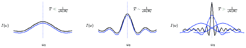
Figure 1: Spectral dependence of one CMB black body mode on sampling interval $T$ (blue line), with $\omega_{0}$ as the epoch frequency, as compared with that of an $\omega=\omega_{0}$ infinite plane wave (black line, the ‘sinc’ function). To comply with the Uncertainty Principle, the two lines follow each other closely until the the CMB mode loses coherence with the plane wave. Beyond that (rightmost graph) the two spectra evolve separately: the central blue curve saturates in height as the Hubble expansion brings other eigenmodes to existence, in the form of further pulses which are part of a periodic sequence. At this point the total CMB spectrum is the sum of all the blue curves.