Fock-space quantum particle approach for the two-mode boson model describing BEC trapped in a double-well potential

Abstract

We develop the Fock-space many-body quantum approach for large number of bosons, when the bosons occupy significantly only few modes. The approach is based on an analogy with the dynamics of a single particle of either positive or negative mass in a quantum potential, where the inverse number of bosons plays the role of Planck constant. As application of the method we consider the Bose-Einstein condensate in a double-well trap. The ground state of positive mass particle corresponds to the mean-field fixed point of lower energy, while that of negative mass to the excited fixed point. In the case of attractive BEC above the threshold for symmetry breaking, the ground state is a cat state and we relate this fact to the double-well shape of the quantum potential for the positive mass quantum particle. The tunneling energy splitting between the local Fock states of the cat state is shown to be extremely small for the nonlinearity parameter just above the critical value and exponentially decreasing with the number of atoms. In the repulsive case, the phase locked ($\pi$-phase) macroscopic quantum self-trapping of BEC is related to the double-well structure of the potential for the negative mass quantum particle. We also analyze the running-phase macroscopic quantum self-trapping state and show that it is subject to quantum collapses and revivals. Moreover, the quantum dynamics just before the first collapse of the running phase shows exponential growth of dispersion of the quantum phase distribution which may explain the growth of the phase fluctuations seen in the experiment on the macroscopic quantum self-trapping.

I Introduction

The fully analytical quantum treatment of a system of interacting $N$ bosons is a hard problem, especially if the number of particles is large, which is usually the case of Bose-Einstein condensate (BEC). In the limit $N\gg 1$ the mean-field approach leads to the Gross-Pitaevskii equation for the order parameter BGL ; PS ; CD . The mean-field limit may be termed “the classical limit” though the Gross-Pitaevskii equation describes non-classical effects, for instance, the quantum coherence of BEC, and reduces to the single-particle Schrödinger equation in the limit of vanishing atomic interaction.

The relation between the full quantum and mean-field dynamics of BEC is a subject of intensive studies. For instance, manifestation of the classical bifurcation in the quantum spectrum of a dimer was studied in Ref. AFKO . The mean-field dynamics of a two-mode model is shown to be modulated by the quantum collapses and revivals MCWW . In Ref. VA ; AV the Bogoliubov-Born-Green-Kirkwood-Yvon hierarchy for statistical operators truncated at the second level was used and it was pointed out that the many-body quantum corrections to the mean-field theory can be identified as decoherence. The correspondence between the many-body quantum dynamics and mean-field (we will also refer to it as a quantum classical correspondence) was also studied in the phase-space by employing Husimi distributions QHAM . The classical-quantum correspondence in the context of quantum collapse and revivals in the nonlinear two and three mode boson models was presented in SK2 ; SK3 , where authors described the BEC interband tunneling between the high-symmetry points of an optical lattice. It was demonstrated that the quantum evolution distinguishes between the stable and unstable classical fixed points, following the classical dynamics about the stable points and diverging from it at the unstable ones. A three-mode boson model was treated in Ref. MJ where a visualization of the eigenstates of the quantum system referring to the underlying classical dynamics was studied.

The purpose of this paper is to propose an analytical method to study the correspondence between the classical and quantum dynamics. We present the relation between the classical fixed points and the eigenenergy states of the full quantum Hamiltonian in the limit of large number of bosons. Our model is based on the simple fact that for $N\gg 1$ the $s$-mode boson model is equivalent to a quantum mechanical dynamics of a single particle living in a compact $(s-1)$-dimensional space. We point out that various quantum features of the system of large number of bosons, not accessible within the mean-field limit, can be derived by the presented method. For instance, one can describe quantum fluctuations, BEC fragmentation (see, for instance, Ref. BECfrag ) and the cat-states formation in the supercritical attractive case BECcats1 ; BECcats2 .

Our method resembles the classical WKB approach to discrete Schrödinger equation, previously developed in another context (see, for instance, the review Braun and the references therein). The discrete WKB quantization method was already applied to the two-mode boson model GK . For instance, it was shown that the semiclassical approximation reproduces the energy eigenvalues even for relatively small $N$.

Our approach is developed in the Fock space, where we expand the exact very complicated Schrödinger equation for the state of $N$-boson system in the small parameter $h=1/N$, the effective Planck constant, reducing it to a much simpler approximate equation resembling that of a single quantum particle in a potential.

In general our method is applicable to $s$-mode boson models. Here we concentrate on the two-mode boson model, reducing it to a one-dimensional Schrödinger equation for the effective quantum particle. We consider the important two-mode model describing BEC in a double-well potential, i.e. the boson Josephson junction model (see, for instance, the reviews Legg ; GO ). BEC in a double well trap is a subject of fundamental experiments and has many potential applications. For instance, it was used for direct observation of the macroscopic quantum tunneling and the nonlinear self-trapping TunTrap , considered as an implementation of the atomic Mach-Zehnder interferometer AtInt ; ThrBif , as a sensitive weak force detector JM ; ChipSens and for preparation of atomic number squeezed states for possible atomic interferometry on a chip AtSqz .

For the two-mode model we find two different Schrödinger equations for description of quantum dynamics about the classical fixed points, corresponding to positive and negative mass of the effective quantum particle. Two reduced Schrödinger equations appear due to the fact that a non-zero classical phase (of the stationary point, in our case) leads to a singularity of the limit $h\to 0$ and, as the result, it appears in the reduced Schrödinger equation. Previously, this has been accounted for by dividing the turning points in the discrete WKB approach into the usual and “unusual” (for details see Ref. Braun ).

The paper is organized as follows. In section II we derive the effective particle representation of the quantum boson Josephson junction model. The two resulting Schrödinger equations for the effective quantum particle are studied in section III. The classical stationary points and their stability properties are studied from the quantum mechanics point of view in section IV. In section V we derive the ground state of the quantum model. In section VI the macroscopic quantum self-trapping (MQST) phenomenon is related to the negative mass effective quantum particle. We also study the quantum dynamics of the running phase MQST states. Section VII contains discussion of the main results. Some of the auxiliary calculations are relegated to appendices A, B, C and D.

II Quantum particle approach for BEC in a double-well trap

Consider, for simplicity, the case of sufficiently weak atomic interaction, when only the degenerate energy levels of the double-well trap are occupied by BEC (we consider the weakly asymmetric double-well with the first two energy levels being quasi-degenerate, $\delta E=E_{2}-E_{1}\ll E_{3}-E_{2}=\Delta E$). Under this condition one arrives at the reduced Schrödinger equation (see also appendix A and Refs. AB ; GO )

$$\frac{i}{N}\partial_{\tau}|\psi\rangle=\hat{H}|\psi\rangle,$$ (1)

$$\hat{H}\equiv\left\{-\frac{1}{N}(a_{1}^{\dagger}a_{2}+a_{2}^{\dagger}a_{1})+\frac{\varepsilon}{N}n_{1}+\frac{\gamma}{N^{2}}(n_{1}^{2}+n_{2}^{2})\right\},$$

where $|\psi\rangle$ is the system state, $n_{j}=a^{\dagger}_{j}a_{j}$ (the boson field operator is expanded over the localized states $\Psi=\varphi_{L}({\bf x})a_{1}+\varphi_{R}({\bf x})a_{2}$) and the time is measured in the tunneling time units: $\tau=t/T$. The parameters of the model are defined as

$$T=\frac{2\hbar}{\delta E},\quad\varepsilon=\frac{2\delta V}{\delta E},\quad\gamma=\frac{gN}{\delta E}\int\mathrm{d}^{3}{\bf x}\,\varphi_{L,R}^{4},$$

$$\delta E=-2\int\mathrm{d}^{3}{\bf x}\,\varphi_{L}\left(-\frac{\hbar^{2}}{2m}\nabla^{2}+V({\bf x})\right)\varphi_{R},$$

$$\delta V=\int\mathrm{d}^{3}{\bf x}\,\left[\varphi_{L}V({\bf x})\varphi_{L}-\varphi_{R}V({\bf x})\varphi_{R}\right].$$ (2)

where $g=4\pi\hbar a_{s}/m$ with $a_{s}$ being the $s$-wave scattering length, $V({\bf x})$ is the double-well potential (centered at zero, for below), the localized states $\varphi_{L}({\bf x})$ and $\varphi_{R}({\bf x})$ are given by the normalized sum and difference of the ground state and the first excited state of the “symmetrized” double-well potential $V_{s}({\bf x})\equiv[V({\bf x})+V(-{\bf x})]/2$ (due to the symmetry the integrals of the fourth power are equal; for more details, see Appendix in Ref. soldw ).

The dimensionless parameter $\delta V$ can be of the same order as $\delta E$, thus $\varepsilon$ can be arbitrary. Note that $\gamma$ is finite (not small) and the applicability condition that the interaction energy is much less than the average trap energy spacing, i.e. $\gamma\ll\Delta E/\delta E$, is satisfied due to the large r.h.s..

Subtracting the conserved quantity $\frac{\gamma}{2N^{2}}(n_{1}+n_{2})^{2}$ from the Hamiltonian in Eq. (1) we obtain the standard representation of the Hamiltonian for the boson Josephson junction (see, for instance, Refs. QHAM ; GO ). Our interaction parameter is related to the standard parameters as follows $\gamma=E_{c}N^{2}/E_{j}$.

We have divided the Schrödinger equation (1) by $N$ and defined the parameters by extracting the explicit $N$-factors reflecting the “order” of the respective boson operators (e.g. $a^{\dagger}_{1}a_{1}\sim N$). This is used in the effective quantum particle representation of Eq. (1) (see Eq. (5)). It is important to observe for the following (and the validity of the explicit $N$-factors) that the physical parameters of the model are $N$-independent in the thermodynamic limit, which is $N\to\infty$ at a constant density $\frac{N}{\Omega}$, where $\Omega$ is the volume. Indeed, $T$ and $\varepsilon$ are evidently constant, while the nonlinear parameter $\gamma\sim\frac{gN}{\delta E\Omega}$ since $|\varphi_{\alpha}|^{4}\sim\Omega^{-2}$.

On the other hand, the factor $N^{-1}$ at the time derivative on the l.h.s. of Eq. (1) plays the rôle of an effective Planck constant and the thermodynamic limit $N\to\infty$ now acquires another meaning, namely it is the semiclassical limit of Eq. (1). To make this clearer, let us rewrite Eq. (1) in the explicit form using the Fock basis

$$|\psi\rangle=\sum_{k=0}^{N}C_{k}|k,N-k\rangle,$$ (3)

where the occupation number corresponding to the left well is denoted by $k$. We get

$$\frac{i}{N}\frac{\mathrm{d}}{\mathrm{d}\tau}C_{k}=-\left(b_{k-1}C_{k-1}+b_{k}C_{k+1}\right)+a_{k}C_{k},$$ (4)

with

$$b_{k}=N^{-1}\left[(k+1)(N-k)\right]^{\frac{1}{2}},$$

$$a_{k}=\gamma N^{-2}\left[k^{2}+(N-k)^{2}\right]+\varepsilon N^{-1}k.$$

Introducing a continuous variable $x=k/N$, the effective Planck constant $h=1/N$ and a wave-function $\Psi(x)=\sqrt{N}C_{k}$ we obtain Eq. (1) in yet another form

$$ih\partial_{\tau}\Psi(x)=-\left\{e^{-i\hat{p}}b_{h}(x)+b_{h}(x)e^{i\hat{p}}\right\}\Psi(x)+a(x)\Psi(x),$$ (5)

with $\hat{p}=-ih\partial_{x}$ and

$$b_{h}(x)=[(x+h)(1-x)]^{1/2},\quad a(x)=\gamma[x^{2}+(1-x)^{2}]+\varepsilon x.$$

Here $x\in(0,1)$ and $\hat{p}$ are canonical variables with the usual commutator $[\hat{p},x]=-ih$ . Note that the inner product for $N\gg 1$ reads $\langle\Psi_{1}|\Psi_{2}\rangle=\int_{0}^{1}\mathrm{d}x\,\Psi^{*}_{1}(x)\Psi_{2}(x)$.

Eq. (5) is written in the $x$-representation form. It can be put in the $\phi$-representation by putting $\hat{p}\to\phi$ and $x-1/2\to ih\partial_{\phi}$ (the shifted variable is more convenient). In a more rigorous way, one can use the transformation of the state vector $C_{k}$ to the Fourier space, given in our case by the discrete Fourier transform,

$$C_{k}=\frac{1}{\sqrt{N+1}}\sum_{l=0}^{N}e^{-ik\phi_{l}}\tilde{C}_{l},\quad\tilde{C}_{l}=\frac{1}{\sqrt{N+1}}\sum_{k=0}^{N}e^{ik\phi_{l}}C_{k},$$ (6)

where $\phi_{l}=2\pi l/(N+1)$. Using periodicity of the exponent we have for $N\gg 1$

$$\Psi(x)=\frac{1}{2\pi}\int\limits_{-\pi}^{\pi}\mathrm{d}\phi\,e^{iN\phi x}\tilde{\Psi}(\phi),\;\tilde{\Psi}(\phi)=N\int\limits_{0}^{1}\mathrm{d}x\,e^{-iN\phi x}\Psi(x),$$ (7)

where $\tilde{\Psi}(\phi_{l})=(N+1)\tilde{C}_{l}$. Thus, for $N\gg 1$ the Hamiltonian for boson Josephson junction in the $\phi$-representation reads (save an inessential constant term)

$$\hat{H} = -2\gamma h^{2}\partial_{\phi}^{2}-\{b_{h}(1/2+ih\partial_{\phi}),\cos(\phi)\}$$ (8)

$$+i\varepsilon h\partial_{\phi}-i[b_{h}(1/2+ih\partial_{\phi}),\sin\phi]$$

where $\{...\}$ denote the anti-commutator. The Hamiltonian (8) reduces to the usual non-rigid pendulum form MFDW if one neglects the variation of $b_{h}(x)$ with respect to $x$.

The limit of large $N$ of Eq. (5) can be considered by the WKB approach for the discrete Schrödinger equation Braun . We write the solution of Eq. (5) in the form $\Psi=\exp\{iS(x,\tau,h)/h\}$ where $S(x,\tau,h)$ is understood as a series $S=S^{(0)}(x,\tau)+hS^{(1)}(x,\tau)+O(h^{2})$ and the terms are assumed to be differentiable functions. In the lowest order we obtain from Eq. (5) the Hamilton-Jacobi equation for the classical action $S^{(0)}(x,\tau)$:

$$-S^{(0)}_{\tau}=a(x)-2b_{0}(x)\cos\left(\frac{\partial S^{(0)}}{\partial x}\right),$$ (9)

where $b_{0}(x)=\sqrt{x(1-x)}$. The classical Hamiltonian obtained from Eq. (9) reads

$$\mathcal{H}=a(x)-2b_{0}(x)\cos\phi$$ (10)

with the canonical variables $x$ and $\phi\in(0,2\pi)$: $\{\phi,x\}=1$ (cf. with Ref. MFDW , where $z=1-2x$). The first-order approximation reads $S^{(1)}=\frac{i}{2}\ln[b_{0}(x)\sin(S^{(0)}_{x})]$.

Let us, however, take a slightly different approach. The most important features of the classical dynamics are the stationary points and their stability properties. About a stationary point (say, $x_{s}$ and $\phi_{s}$) the classical action can be expanded as follows

$$S^{(0)}(x,\tau)=-E^{(cl)}\tau+\phi_{s}(x-x_{s})+O[(x-x_{s})^{2}],$$ (11)

where we have used that $S^{(0)}(x,\tau)=-E^{(cl)}\tau+S^{(st)}(x)$ and $\frac{\partial S^{(st)}}{\partial x}(x_{s})=\phi_{s}$. We are interested in the limit of large $N$. The wave-function localized about some $x_{s}$-point has a singular derivative in the limit $h\to 0$: $\frac{\partial\Psi}{\partial x}\sim ih^{-1}\phi_{s}\Psi(x,\tau)$ if $\phi_{s}\neq 0$. The singularity is due to the classical phase in the wave-function. We then account for the phase explicitly, introducing the transformation (at some $x_{s}$-point)

$$\Psi(x,\tau)=e^{iN\phi(\tau)(x-x_{s})}\psi(x,\tau)$$ (12)

before taking the limit of large $N$. The phase $\phi(\tau)$ satisfies the evolution equation $\dot{\phi}=\partial H(x_{s},\phi)/\partial x$ (by expanding the Schrödinger equation in $x-x_{s}$ and taking the limit $h\to 0$), hence it is nothing but the classical phase.

To obtain a reduced Schrödinger equation we substitute the representation (12) into Eq. (5) and expand the result into series in $\hat{p}$ keeping the terms up to $O(\hat{p}^{2})$ (since the derivative is regular the expansion is actually in $h$). We have

$$\left\{e^{-i\hat{p}}b_{h}(x)+b_{h}(x)e^{i\hat{p}}\right\}e^{i\frac{\phi}{h}x}\psi(x) = e^{i\frac{\phi}{h}x}\biggl{\{}2\cos(\phi)b_{h}(x)-h\cos(\phi)\frac{\mathrm{d}b_{h}}{\mathrm{d}x}-\sin\phi\left[\hat{p}b_{h}(x)+b_{h}(x)\hat{p}\right]$$ (13)

$$-\frac{1}{2}\left[e^{-i\phi}\hat{p}^{2}b_{h}(x)+e^{i\phi}b_{h}(x)\hat{p}^{2}\right]+O(\hat{p}^{3})\biggr{\}}\psi(x).$$

One can make one more reduction in Eq. (13) by using that

$$\frac{1}{2}\left[e^{-i\phi}\hat{p}^{2}b_{h}+e^{i\phi}b_{h}\hat{p}^{2}\right]=\cos(\phi)\hat{p}b_{h}\hat{p}$$

$$-\frac{1}{2}\left\{h\sin\phi\left(\frac{\mathrm{d}b_{h}}{\mathrm{d}x}\hat{p}+\hat{p}\frac{\mathrm{d}b_{h}}{\mathrm{d}x}\right)+\frac{h^{2}}{2}\cos(\phi)\frac{\mathrm{d}^{2}b_{h}}{\mathrm{d}x^{2}}\right\}.\qquad$$ (14)

Using Eqs. (13) and (14) in the Schrödinger equation (5) we obtain

$$ih\partial_{\tau}\psi=\mathcal{V}_{h}(x,\phi)\psi+\Bigl{[}\cos\phi\,\hat{p}b_{h}(x)\hat{p}+\sin\phi\left(b_{h}(x)\hat{p}+\hat{p}b_{h}(x)\right)-\frac{h}{2}\sin\phi\left(\frac{\mathrm{d}b_{h}}{\mathrm{d}x}\hat{p}+\hat{p}\frac{\mathrm{d}b_{h}}{\mathrm{d}x}\right)\psi+O(\hat{p}^{3})\Bigr{]}\psi,$$ (15)

where the potential $V_{h}$ reads

$$\mathcal{V}_{h}=a(x)-2b_{h}(x)\cos\phi+h\cos\phi\left[\frac{\mathrm{d}b_{h}}{\mathrm{d}x}-\frac{h}{4}\frac{\mathrm{d}^{2}b_{h}}{\mathrm{d}x^{2}}\right].$$ (16)

Reducing further, one can neglect the terms of order $O(h)$ in the potential $\mathcal{V}_{h}$, since it contains the $h$-independent term, obtaining nothing but the classical Hamiltonian (10) $\mathcal{V}_{0}(x)=\mathcal{H}=a(x)-2b_{0}(x)\cos\phi$.

The analogy with the quantum problem of a particle in a potential becomes evident from the Schrödinger equation in the form of Eq. (15). The stationary states $\psi(x,\tau)=e^{-iE\tau/h}\psi_{E}(x)$ correspond to the extrema of the quantum potential. The extremal values of the classical phase (which is a parameter) given by $\frac{\partial\mathcal{V}_{0}(x,\phi)}{\partial\phi}=0$ coincide with the classical values at the stationary points: $\phi=0$ or $\phi=\pi$. These correspond to positive or negative mass of the effective quantum particle.

III Quantum model about the mean-field stationary points

The Schrödinger equation (15) in the two cases $\phi_{+}=0$ and $\phi_{-}=\pi$ reduces to

$$ih\partial_{\tau}\psi=\left\{\pm\hat{p}\sqrt{x(1-x)}\hat{p}+\mathcal{V}_{\pm}(x)\right\}\psi,$$ (17)

where the upper/lower sign corresponds to $\phi_{+}/\phi_{-}$ and $\mathcal{V}_{\pm}(x)=\gamma[x^{2}+(1-x)^{2}]+\varepsilon x\mp 2\sqrt{x(1-x)}$. For further analysis it is convenient to introduce a new variable $z=1-2x$, the atomic population difference divided by the total number of atoms. We get

$$ih\partial_{\tau}\psi=\left\{\mp 2h^{2}\frac{\mathrm{d}}{\mathrm{d}z}\sqrt{1-z^{2}}\frac{\mathrm{d}}{\mathrm{d}z}+V_{\pm}(z)\right\}\psi,$$ (18)

where the potential simplifies to

$$V_{\pm}(z)=\frac{1}{2}(\gamma{}z^{2}-\varepsilon{}z)\mp\sqrt{1-z^{2}}.$$ (19)

Note that the potential $V_{\pm}(z)$ crucially depends on the nonlinearity parameter $\gamma$.

Taking into account the symmetry of Eq. (18) with respect to replacing $\pm$ we have the following mapping between the repulsive and attractive BEC cases:

$$\gamma_{\mathrm{attr}}=-\gamma_{\mathrm{rep}},\quad z_{\mathrm{attr}}=-z_{\mathrm{rep}},$$

$$\psi_{\mathrm{attr}}(z,\tau;\gamma,\phi_{\pm})=\psi^{*}_{\mathrm{rep}}(-z,\tau;-\gamma,\phi_{\mp}),$$ (20)

i.e., for instance, an attractive BEC with positive mass $\phi=0$ is equivalent to a repulsive BEC with negative mass $\phi=\pi$ evolving backwards in time in the inverted space $z\to-z$. Note that it is sufficient to consider also $\varepsilon\geq 0$, since $\varepsilon<0$ can be simulated by replacing $z\to-z$.

The equivalence (20), however, is useful only in the general analytical analysis, the attractive BEC is fundamentally different from the repulsive BEC. As we show below, in both cases the Schrödinger equation (18) with the positive mass gives the ground state of BEC and only in the attractive case $V_{+}(z)$ has the double-well form (see Fig. 1(a) below).

The extrema of the potential (19) solve the equation

$$\gamma\pm\frac{1}{\sqrt{1-z^{2}}}=\frac{\varepsilon}{2z}.$$ (21)

Consider $\gamma>0$, $\varepsilon\geq 0$. In the case of positive mass ($\phi=0$) there is just one minimum. For the case of negative mass ($\phi=\pi$) there is a critical $\gamma_{\mathrm{cr}}$ below which there is just one solution which is a minimum of $V=-V_{-}(z)$, whereas for $\gamma>\gamma_{\mathrm{cr}}$ there are three solutions, two corresponding to local minima and one to a local maximum, see Fig. 1(a). Eq. (21) is easily solved graphically by plotting the l.h.s. and the r.h.s. as functions of $z$, see Fig. 1(b). Hence, in the case of $\phi=0$ (the upper sign) we get that the positive-mass effective quantum particle moves in a single well potential $V=V_{+}(z)$ and there is only one solution to Eq. (21). In the case of $\phi=\pi$ the negative-mass particle sees either one well or two well potential $V=-V_{-}(z)$.

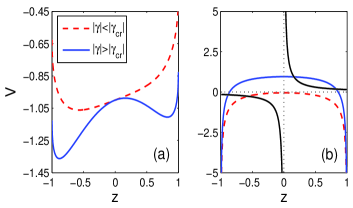
Figure 1: (Color online) The potential for the effective quantum particle, panel (a), (here $V=-V_{-}(z)$ for the repulsive BEC corresponding to negative mass, $\phi=\pi$, or $V=V_{+}(-z)$ for the attractive BEC for $\phi=0$, positive mass) and the graphical solution of Eq. (21), panel (b) (again for $\phi=\pi$ for the repulsive BEC, or for $\phi=0$ for the attractive BEC, in the last case the axes are inverted). Here $\varepsilon=0.3$ which gives $|\gamma_{\mathrm{cr}}|=1.4521$.

The critical value of the nonlinearity coefficient can be found by equating the derivatives of the two sides of Eq. (21), which gives an additional equation. We get

$$\gamma_{\mathrm{cr}}=\left[1+\left(\frac{\varepsilon}{2}\right)^{\frac{2}{3}}\right]^{\frac{3}{2}},$$ (22)

while the corresponding solution, i.e. the point of inflection, reads $z_{\mathrm{cr}}=[1+(2/\varepsilon)^{2/3}]^{-1/2}$. For $\gamma>\gamma_{\mathrm{cr}}$ two positive solutions bifurcate from it: $z_{1}<z_{\mathrm{cr}}<z_{2}$, where $z_{1}$ is the local maximum of the inverted potential $-V_{-}(z)$. The local maximum solution is an analog of the $z=0$ solution for $\varepsilon\neq 0$.

One can show (see Appendix B) that in the case of $\phi=\pi$ the negative local minimum of the inverted quantum potential is also the absolute minimum (of this potential, i.e. $-V_{-}(z)$) for all $\gamma>\gamma_{\mathrm{cr}}$ and $\varepsilon\geq 0$, whereas the negative $z$ correspond to higher atomic population of the trap well with the higher zero-point energy (see Eq. (1)). This fact, however, is easily explained within our approach by the negative mass of the effective quantum particle.

Finally, all the results obtained for the repulsive BEC are transferred to the attractive BEC case by using the equivalence given in Eq. (20). For instance the cases of $\phi_{\pm}$ are interchanged and the double-well potential of Fig. 1(a) in the case of attractive BEC appears for $\phi=0$ (i.e. now $V=V_{+}(-z)$) and $\gamma<-\gamma_{\mathrm{cr}}=-\left[1+\left(\frac{\varepsilon}{2}\right)^{2/3}\right]^{3/2}$.

IV The mean-field stationary points and their stability explained

Before we proceed with the analysis of the bound state wave-functions, let us explain from the quantum mechanical point of view the appearance and stability properties of the stationary points of the classical Hamiltonian (see also Ref. MFDW ). In the new variables we have

$$\mathcal{H}=\frac{\gamma}{2}z^{2}-\frac{\varepsilon}{2}z-\sqrt{1-z^{2}}\cos\phi,$$ (23)

where one must remember that $\{\phi,z\}=-2$. The stationary points of the classical Hamilton equations, $\dot{z}=-2\frac{\partial\mathcal{H}}{\partial\phi}$, $\dot{\phi}=2\frac{\partial\mathcal{H}}{\partial z}$, correspond to the extrema of the quantum potential ${V}(z)$, i.e. $\cos\phi_{s}=\pm 1$, whereas $z_{s}$ is defined from Eq. (21). Consider the case $\gamma>0$ (repulsive BEC) and $\varepsilon\geq 0$. The stability properties are defined by the local Hamiltonian, see also Fig. 2. Introduce the local phase space co-ordinates $\phi=\phi_{s}+\varphi$ and $z=z_{s}+\zeta$.

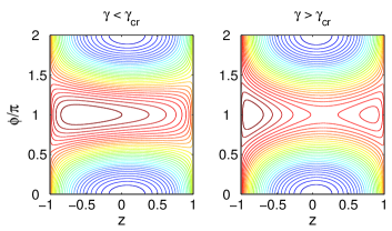
Figure 2: (Color online) The phase portrait of the classical Hamiltonian Eq. (23) corresponding to a repulsive BEC in a double-well trap. The parameters are as in Fig. 1.

1. In the case of $\phi_{s}=0$ we have up to the second-order terms in the local variables

$$\mathcal{H}_{+}=V_{+}(z_{s})+\sqrt{1-z_{s}^{2}}\frac{\varphi^{2}}{2}+\left[\gamma+(1-z_{s}^{2})^{-3/2}\right]\frac{\zeta^{2}}{2},$$ (24)

hence the classical stationary point $\phi_{s}=0$ and $z=z_{s}$, solving Eq. (21) for the upper sign, is elliptic and stable. This stationary point, in fact, corresponds to the absolute minimum of the quantum potential $V_{+}(z)$.

2. In the case of $\phi_{s}=\pi$ we obtain up to the second-order terms (by simply changing the sign at $\cos\phi$)

$$\mathcal{H}_{-}=V_{-}(z_{s})-\sqrt{1-z_{s}^{2}}\frac{\varphi^{2}}{2}-\left[(1-z_{s}^{2})^{-3/2}-\gamma\right]\frac{\zeta^{2}}{2}.$$ (25)

First, consider the solution to Eq. (21) such that $z_{s}<0$. Using Eq. (21) in the following estimate

$$\gamma-\frac{1}{(1-z_{s}^{2})^{3/2}}<\frac{\gamma}{1-z_{s}^{2}}-\frac{1}{(1-z_{s}^{2})^{3/2}}$$

$$=\frac{\varepsilon}{2z_{s}(1-z_{s}^{2})}<0,$$

we conclude that the negative stationary point $z_{s}<0$ for $\phi_{s}=\pi$ is always elliptic and hence stable. It actually corresponds to the absolute minimum of $-V_{-}(z)$ (see Appendix B).

Now consider the positive stationary points $z^{(1)}_{s}<z_{\mathrm{cr}}<z^{(2)}_{s}$, which appear for $\gamma>\gamma_{\mathrm{cr}}$. For $z^{(1)}_{s}$ we have

$$\gamma-\frac{1}{\left(1-[z^{(1)}_{s}]^{2}\right)^{3/2}}>\gamma-\frac{1}{(1-z_{\mathrm{cr}}^{2})^{3/2}}=\gamma-\gamma_{\mathrm{cr}}>0,$$

where we have used that $\gamma_{\mathrm{cr}}=(1-z_{\mathrm{cr}}^{2})^{-3/2}$. Thus this stationary point is hyperbolic and hence unstable (recall that it corresponds to the local maximum of $-V_{-}(z)$). The other stationary point $z^{(2)}_{s}>z_{\mathrm{cr}}$ is a local minimum of the quantum potential $-V_{-}(z)$. Let us show that it is always elliptic, i.e. stable. Indeed, using Eq. (21) we obtain the estimate ($z=z^{(2)}_{s}$)

$$\gamma-\frac{1}{(1-z^{2})^{3/2}}=\left(\gamma-\frac{1}{\sqrt{1-z^{2}}}\right)\frac{1}{1-z^{2}}-\frac{\gamma z^{2}}{1-z^{2}}$$

$$=\frac{1}{1-z^{2}}\left(\frac{\varepsilon}{2z}-\gamma z^{2}\right)=-\frac{z^{2}}{1-z^{2}}\left[\gamma-\frac{\varepsilon}{2z^{3}}\right]<0,$$ (26)

where we have used that $z^{(2)}_{s}>z_{\mathrm{cr}}$, the expression $\gamma_{\mathrm{cr}}={\varepsilon}/(2z^{3}_{\mathrm{cr}})$ and that $\gamma>\gamma_{\mathrm{cr}}$.

According to Eq. (20), the classical action for Eq. (18) satisfies $S^{(0)}_{\mathrm{attr}}(z,\tau)=-S^{(0)}_{\mathrm{rep}}(-z,\tau)$ where $\gamma\to-\gamma$ and $\phi_{\pm}\to\phi_{\mp}$, thus Eqs. (24) and (25) can be transferred to an attractive BEC by the substitution: $-\mathcal{H}_{\pm}\to\mathcal{H}_{\mp}$ and $-V_{\pm}\to V_{\mp}$.

In conclusion of this section, the local minima of the quantum potential (or the inverted potential, in the case of negative mass) correspond to the elliptic stationary points of the classical dynamics and the local maximum to a hyperbolic stationary point, which is a physically clear result.

V The ground state of BEC in a double-well trap

To find the ground state of BEC in the double-well trap one has to analyze the energy of the bound states localized at the extrema of the potentials $V_{\pm}(z)$. For $N\gg 1$ one needs to compare just the zero-point energies at the extremal points (which is the classical energy of the stationary point, Eqs. (24) and (25)). The result is that for both attractive and repulsive BEC in a double-well trap the ground state is given by that of the effective quantum particle with the positive mass, i.e. with the classical phase $\phi=0$ (see appendix C for details).

The direct link between the stable classical stationary points and the nature of the corresponding quantum states discussed in section IV allows one to get the local approximation for the quantum bound states by directly quantizing the local Hamiltonian, Eqs. (24) and (25), by replacing $\varphi\to 2ih\partial_{\zeta}$, since $[\hat{\varphi},\zeta]=2ih$ (remembering that in the case of attractive BEC Eq. (24) corresponds to $\phi=\pi$, while Eq. (25) to $\phi=0$). We slightly correct this scheme in the negative mass case, where the wave function $\Psi(x,t)$ of BEC in a double-well trap has a non-trivial phase according to Eq. (12).

Writing the local classical Hamiltonian in Eqs. (24)-(25) as

$$H_{\pm}(\zeta,\varphi)=V_{\pm}(z_{s})+(a_{\pm}\varphi^{2}+b_{\pm}\zeta^{2})/2,$$ (27)

we obtain an approximation to the bound state of BEC corresponding to a stable stationary point of the classical dynamics and its energy as follows:

$$\Psi_{\mathcal{E}_{\pm}}(x)=\frac{1}{\pi^{1/4}\sigma_{\pm}^{1/2}}\exp\left\{i\frac{\phi_{\pm}}{h}x-\frac{(x-x_{s})^{2}}{2\sigma_{\pm}^{2}}\right\},$$

$$\mathcal{E}_{\pm}=V_{\pm}(z_{s})+O(h),$$ (28)

where $\sigma_{\pm}^{2}=\frac{1}{2N}\sqrt{\frac{a_{\pm}}{b_{\pm}}}$ is the Gaussian width and we have used that $\Delta z=2\Delta x$. The energy spacing for the few lower levels reads $\Delta\mathcal{E}_{\pm}=h\Omega_{\pm}$, where $\Omega_{\pm}=2\sqrt{a_{\pm}b_{\pm}}$ is the classical frequency. In the case of negative mass the energy levels of a local quantum Hamiltonian are descending.

V.1 The ground state of repulsive BEC

For $\gamma>0$ we obtain the single solution of Eq. (21) corresponding to the positive mass case in the form of a series in $\varepsilon$:

$$z_{s}=\frac{\varepsilon}{2}(1+\gamma)^{-1}\left[1-\frac{\varepsilon^{2}}{8(1+\gamma)^{3}}+O(\varepsilon^{4})\right],$$ (29)

which is valid for a weakly asymmetric potential $V_{+}(z)$, i.e. $\varepsilon\ll 1+\gamma$. The average atomic population difference between the two wells reads $\langle n_{1}-n_{2}\rangle=z_{s}N$. By the substitution $\gamma\to-\gamma$ and $z_{s}\to-z_{s}$ Eq. (29) also gives the position of the minimum of the inverted potential $-V_{-}(z)$ in the subcritical case $\gamma<\gamma_{\mathrm{cr}}$.

For a weakly asymmetric potential $V_{+}(z)$ one can also calculate the atom number fluctuations using the local approximation for the ground state given by Eq. (28) ($x_{s}=(1-z_{s})/2$):

$$\langle\Delta n_{1}^{2}\rangle=N^{2}\langle(x-x_{s})^{2}\rangle=\frac{N^{2}\sigma_{+}^{2}}{2}$$

$$\quad=\frac{N}{4}(1+\gamma)^{-1/2}\left[1-\frac{\varepsilon^{2}(4+\gamma)}{16(1+\gamma)^{3}}+O(\varepsilon^{4})\right],\quad$$ (30)

where we have used that

$$\sigma^{2}_{+}=\frac{1}{2N}\left[\frac{(1-z_{s})^{1/2}}{\gamma+(1-z_{s}^{2})^{-3/2}}\right]^{1/2}$$ (31)

and the series expression (29) (see the details in Appendix D).

The result given by Eqs. (28) and (30) can be compared to the non-interacting case, which is exactly solvable (here we consider the case $\varepsilon=0$). Indeed, the tunneling term of the quantum Hamiltonian (1) can be diagonalized by the canonical transformation $c_{\pm}=(a_{1}\pm a_{2})/\sqrt{2}$ with the effect $H=-(a_{1}^{\dagger}a_{2}+a_{2}^{\dagger}a_{1})/N=(c_{-}^{\dagger}c_{-}-c_{+}^{\dagger}c_{+})/N$. The eigenstates are given by $(c_{+}^{\dagger})^{m}(c_{-}^{\dagger})^{N-k}|0,0\rangle$, where $a_{1}|0,0\rangle=a_{2}|0,0\rangle=0$. The ground state corresponds to $m=N$

$$|\Phi\rangle=\frac{1}{\sqrt{2^{N}N!}}\left(a_{1}^{\dagger}+a_{2}^{\dagger}\right)^{N}|0,0\rangle,$$ (32)

For large $N$, approximating the factorial, we get the coherent state in the Fock basis as

$$\Phi(z) = \sqrt{N}\langle\frac{1-z}{2}N,\frac{1+z}{2}N|\Phi\rangle$$ (33)

$$= \left(\frac{2N}{\pi}\right)^{\frac{1}{4}}\exp\left\{-\frac{N}{4}\left(z^{2}+\frac{z^{4}}{6}+...\right)\right\}.$$

Eqs. (28) - (30) describe all three known regimes of repulsive BEC tunneling in the double-well trap (see for instance, Ref. Legg ; GO ): (1) Rabi regime, when the coherence is very high and the atom number fluctuations are large (essentially the interaction free regime), $\gamma\ll 1$; (2) Josephson regime, when the coherence is high and the atom number fluctuations are small, $1\ll\gamma\ll N^{2}$ and (3) Fock regime, when the coherence is low and the atom number fluctuations vanish, $\gamma\gg N^{2}$.

V.2 The ground state of attractive BEC

Subcritical $\gamma$. In the case $|\gamma|<\gamma_{\mathrm{cr}}$ the ground state of attractive BEC is essentially the same as that of the repulsive BEC and is given by the general result (28) for the positive mass case (i.e. the upper sign). The average population difference is again given by the series solution (29) and the number fluctuations are given by the same formula (30) as in the repulsive case. However, since now $\gamma<0$, there is an essential difference: even moderate attractive interactions strongly enhance the atom number fluctuations (which fact leads to absence of the Josephson regime for attractive BEC).

For $\gamma$ approaching (from above) the critical value $-\gamma_{\mathrm{cr}}$ the fluctuations given by the local oscillator approximation (28) diverge, which is easily seen from Eq. (30) applied to the case $\varepsilon=0$. In the general case the result is similar and follows from the exact expression for $\sigma^{2}_{+}$ with the use of the exact value for the point of inflection $z_{s}$ (given below Eq. (22) of section III) and the expression $\gamma_{\mathrm{cr}}=(1-z_{\mathrm{cr}}^{2})^{-3/2}$ . The divergence results from the oscillator approximation of the wave-function $\Psi(x)$ (28) which breaks down at the critical value of $\gamma$, since the potential $V_{+}(z)$ for $\gamma=-\gamma_{\mathrm{cr}}$ is approximated about the stationary point $z=z_{s}$ by the fourth order power in $z-z_{s}$ (we give the case $\varepsilon=0$ and $z_{s}=0$ for simplicity):

$$V_{+}(z)=-\frac{z^{2}}{2}-\sqrt{1-z^{2}}=\frac{z^{4}}{8}+\frac{z^{6}}{16}+....$$ (34)

Hence, the usual oscillator approximation should be replaced about the critical $\gamma$ by the ground state in the non-harmonic potential, not known in the exact form.

Supercritical $\gamma$. In the general case of $|\gamma|>\gamma_{\mathrm{cr}}$ one has to solve the stationary Schrödinger equation (18) to obtain the ground state. However, for $\gamma$ such that the potential $V_{+}(z)$ is a double-well with well-separated wells (the form of this potential is essentially determined by the atomic interaction parameter), the oscillator approximation is still valid locally (i.e. about the two minima of the potential $V_{+}(z)$, see Fig. 1) and the ground state can be now approximated by a combination of the local eigenfunctions of the form (28) due to the quantum tunneling between the wells of $V_{+}(z)$.

The case $\varepsilon=0$ is the most interesting. The two local minima, solutions of Eq. (21), read $z^{(\pm)}_{s}=\pm\sqrt{1-\gamma^{-2}}$. The validity of the local approximation by oscillator eigenfunctions in the two wells, i.e. the condition of well-separated wells of the potential $V_{+}(z)$ for $\gamma<-1$, is defined by how much the width of the local oscillator eigenfunctions is smaller than the distance between the two wells. We have $z_{R}-z_{L}=2\sqrt{1-\gamma^{-2}}$ and using Eq. (28) $\langle(z-z_{L})^{2}\rangle=4\langle(x-x_{L})^{2}\rangle=N^{-1}|\gamma|^{-1}(\gamma^{2}-1)^{-1/2}$. Therefore, the applicability condition $\langle(z-z_{L})^{2}\rangle\ll(z_{R}-z_{L})^{2}/4$ reads

$$|\gamma|(|\gamma|-|\gamma|^{-1})^{3}\gg\frac{1}{N^{2}},$$ (35)

where on the l.h.s. we have a monotonically growing function of $|\gamma|$. The condition is not too restrictive and already for $|\gamma|$ slightly above the critical value $|\gamma|=1$ it is satisfied, e.g. setting $|\gamma|=1+\delta$ with $\delta\ll 1$ in Eq. (35) we obtain $\delta\gg N^{-2/3}$ which for $N=1000$ gives $\delta\gg 0.01$. Hence already $|\gamma|=1+\delta\geq 1.1$ satisfies the condition (35) for $N=1000$.

To obtain the ground state we need to evaluate the tunneling rate, i.e. the matrix element $\langle\Psi_{L}|\hat{H}|\Psi_{R}\rangle$, where for the localized eigenfunctions in the left and right well of the double well $V_{+}(z)$ one can use the local approximation (28) and $\hat{H}$ can be taken from Eq. (18). We have for the localized states in the left and right wells (here $s=L,R$)

$$\Psi_{s}(z)=\frac{1}{\pi^{1/4}\sqrt{\sigma}}e^{-\frac{(z-z_{s})^{2}}{2\sigma^{2}}},$$ (36)

where $\sigma^{2}=4\sigma_{+}^{2}=\frac{2}{N}|\gamma|^{-1}(\gamma^{2}-1)^{-1/2}$. Note that there is an exponentially small overlap between $\Psi_{L}$ and $\Psi_{R}$:

$$\langle\Psi_{L}|\Psi_{R}\rangle = \frac{1}{\sqrt{\pi}\sigma}\int\limits_{-1}^{1}\mathrm{d}z\,\exp\{-\frac{(z-z_{L})^{2}+(z-z_{R})^{2}}{2\sigma^{2}}\}$$ (37)

$$= \exp\left\{-\frac{N}{2}|\gamma|^{-1}(\gamma^{2}-1)^{3/2}\right\},$$

where we have used that $(z-z_{L})^{2}+(z-z_{R})^{2}=2(z^{2}+z_{L}^{2})$ and the normalization of the function $\Psi(z)=\pi^{-1/4}\sigma^{-1/2}\exp\{-\frac{z^{2}}{2\sigma^{2}}\}$. Using the integration by parts we get

$$\langle\Psi_{L}|\hat{H}|\Psi_{R}\rangle = \frac{2}{\sigma^{4}N^{2}}\langle\Psi_{L}|(z-z_{L})(z-z_{R})\sqrt{1-z^{2}}|\Psi_{R}\rangle$$

$$+\langle\Psi_{L}|\gamma z^{2}/2-\sqrt{1-z^{2}}|\Psi_{R}\rangle.$$

To estimate the products we use $(z-z_{L})(z-z_{R})=z^{2}-1+\gamma^{-2}$ and set $z=0$ where the overlap of the wave-functions $\Psi_{L,R}(z)$ is maximal, with the effect

$$\langle\Psi_{L}|\hat{H}|\Psi_{R}\rangle\approx-\left[1+\frac{(\gamma^{2}-1)^{2}}{2}\right]\langle\Psi_{L}|\Psi_{R}\rangle.$$ (38)

It is natural to define the “tunneling coefficient” $\kappa$ for the effective quantum particle as follows (cf. with Eq. (2))

$$\kappa = -\langle\Psi_{L}|\hat{H}|\Psi_{R}\rangle$$

$$\approx \left[1+\frac{(\gamma^{2}-1)^{2}}{2}\right]\exp\left\{-\frac{N}{2|\gamma|}(\gamma^{2}-1)^{3/2}\right\}.$$

The ground and first excited states in the supercritical double-well potential $V_{+}(z)$ for $\gamma<0$ read

$$|G\rangle=\frac{1}{\sqrt{2}}(|\Psi_{L}\rangle+|\Psi_{R}\rangle),\;|E\rangle=\frac{1}{\sqrt{2}}(|\Psi_{L}\rangle-|\Psi_{R}\rangle),$$ (40)

where $\Psi_{L,R}(z)$ are given by Eq. (36). The theoretical ground state is a very good approximation of the numerical diagonalization of the quantum Hamiltonian (1), see Fig. 3.

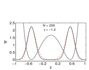
Figure 3: (Color online) The ground state of attractive BEC in the supercritical case: theoretical (given by Eqs. (36) and (40), solid line) vs. numerical diagonalization of the Hamiltonian (dashed line). The thick grey line shows schematically the effective potential $V_{+}(z)$. Here $N=200$, $\gamma=-1.2$ and $\varepsilon=0$.

The degenerate level energy splitting, given by $\delta E=2\kappa$, is a qualitatively good result, see Fig. 4. Note that the $N$-dependence of the energy duplet splitting is manifestly exponential (however, the local approximation used for the wave functions cannot capture the right coefficient in the exponent). The energy splitting can be also estimated by using the perturbation theory, but only for small values of $N$ (since the small parameter is equivalent to $N/\gamma$ see, for details, Ref. BES ).

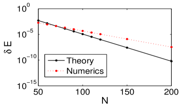
Figure 4: (Color online) The energy splitting due to tunneling in the effective potential well vs. number of atoms $N$: theoretical (solid line) and numerical (dotted line). Here $\gamma=-1.2$ and $\varepsilon=0$.

The atom number fluctuations in the ground state (40) read

$$\langle\Delta n_{1}^{2}\rangle=\frac{N^{2}}{4}\langle G|z^{2}|G\rangle\approx\frac{N^{2}}{4}(1-\gamma^{-2}).$$ (41)

For large $|\gamma|$ above the critical value the ground state of an attractive BEC in the symmetric double-well trap is the Schrödinger cat-state (see also Refs. BECcats1 ; BECcats2 ). Precisely, for $|\gamma|\gg\sqrt{N}$ we have

$$|G\rangle=\frac{1}{\sqrt{2}}(|N,0\rangle+|0,N\rangle).$$ (42)

Indeed, in the supercritical case $\Psi_{L,R}(z)$, given by Eq. (36), has the width in the Fock space given by $N\sqrt{\langle(z-z_{s})^{2}\rangle}/2=\frac{\sqrt{N}}{2}|\gamma|^{-1/2}(\gamma^{2}-1)^{-1/4}\approx\sqrt{N}/(2|\gamma|)\ll 1$ for $|\gamma|\gg\sqrt{N}$. Thus each state $|\Psi_{L,R}\rangle$ is a Fock state.

VI MQST and the negative mass quantum particle

The equivalence between the repulsive and attractive BEC cases, given by Eq. (20), means, for instance, that the repulsive BEC also contains the Schrödinger cat-state (see also Ref. GE ), which is an excited stationary state.

The double-well potential $V=V_{-}(z)$ for the classical phase $\phi=\pi$ is responsible for the MQST states of a repulsive BEC in a symmetric double-well, predicted in Ref. MFDW and observed experimentally in Ref. TunTrap . There are two types of the MQST: the phase-locked ($\phi\approx\pi$) states and the running phase states ($\phi\propto t$). Consider the symmetric double-well trap ($\varepsilon=0$). Following the arguments of Ref. MFDW in the classical case, i.e. using $\mathcal{H}=E$ and Eq. (23) one arrives at the equation

$$\frac{1}{4}\left(\frac{\mathrm{d}z}{\mathrm{d}\tau}\right)^{2}=1-z^{2}-\left(\frac{\gamma}{2}z^{2}-E\right)^{2},$$ (43)

which results in inaccessible $z=0$ region for $|E|>1$. Since for $N\gg 1$ the energy satisfies $V_{+}(z)\leq E\leq V_{-}(z)$, this is possible only when the potential $V_{-}(z)=\frac{\gamma}{2}z^{2}+\sqrt{1-z^{2}}$ has a local minimum at $z=0$ (i.e. it is an inverted double-well) and the energy line crosses it. Hence, the MQST is possible only for $\gamma>1$. The mean-field condition for the MQST reads $\gamma>\gamma_{\mathrm{c}}$ where MFDW

$$\gamma_{\mathrm{c}}=2\frac{1+\sqrt{1-z^{2}(0)}\cos[\phi(0)]}{z^{2}(0)}.$$ (44)

One can easily verify that the mean-field critical value always satisfies $\gamma_{\mathrm{c}}>1$, which is easily seen by rewriting Eq. (44) as $\gamma z(0)^{2}/2=1+\sqrt{1-z(0)^{2}}\cos{\phi(0)}$ and noticing that if $\gamma\leq 1$ the functions on the l.h.s. and on the r.h.s. have no intersections for $0<|z(0)|<1$. Note that for $\cos\phi(0)\geq 0$ we get $\gamma_{\mathrm{c}}\geq 2$. For $\gamma>2$ the MQST condition reads $|z(0)|>z_{c}$ where $z_{c}$ is the solution of Eq. (44). On the other hand, for $\cos\phi(0)<0$ and $1+|\sin\phi(0)|<\gamma<2$ there is an interval of the initial population imbalance for MQST: $z_{1}<|z(0)|<z_{2}$, where $z_{1,2}$ solve Eq. (44).

If repulsive BEC is prepared in one well of the double-well trap and the initial phase $\phi(0)\approx\pi$ one can use the negative mass Schrödinger equation (18) to explain the quantum dynamics. In this case the quantum potential in the Fock space $V=V_{-}(z)$ has the double-well form with the quasi-degenerate energy levels, which reflect the existence of two classical fixed points $z_{s}^{(\pm)}=\pm\sqrt{1-\gamma^{-2}}$. The degeneracy is estimated as twice the tunneling coefficient of Eq. (V.2). Therefore, the observation of the mean-field MQST with phase $\langle\phi\rangle\approx\pi$ is subject to the quantum condition that the oscillation time of the effective quantum particle in one of the wells is much less than the tunneling time between the wells of the double-well potential $V_{-}(z)$, i.e. in the energy terms $2\kappa\ll h\Omega_{-}=2h\sqrt{a_{-}b_{-}}$ or

$$\left[1+\frac{(\gamma^{2}-1)^{2}}{2}\right]\exp\left\{-\frac{N}{2\gamma}(\gamma^{2}-1)^{3/2}\right\}\ll\frac{\sqrt{\gamma^{2}-1}}{N},$$ (45)

which, as is demonstrated in Fig. 5, is satisfied for all $\gamma$ just above the critical value, even for small number of BEC atoms. This fact makes possible the experimental observation of the phase-locked mean-field MQST. A similar conclusion was made before using different approach ST ; RSK . We note also that the $\pi$-phase MQST was analyzed in Ref. ST by considering the numerical eigenvalue spectrum (see also Ref. GE ) and was related to the appearance of the quasi-degenerate energy doublets.

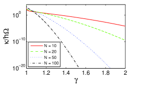
Figure 5: (Color online) An illustration of the quantum condition, i.e. $\kappa/h\Omega_{-}\ll 1$, for the phase-locked MQST states for several values of the number of BEC atoms $N$.

Numerical simulations show that the quantum average values defined as

$$\!\!\!\langle z\rangle=1-\frac{2}{N}\sum_{k=0}^{N}k|C_{k}|^{2},\;\langle\phi\rangle=\textrm{arg}\langle e^{i\hat{p}}\rangle=\textrm{arg}\sum_{k=0}^{N-1}C^{*}_{k}C_{k+1},$$ (46)

initially follow the mean-field dynamics, see Fig. 6. The atomic distribution in the Fock space remains localized in one of the wells of the inverse quantum potential $-V_{-}(z)$, Fig. 7(a). The distributed quantum phase $\phi_{k}$, defined as $\phi_{k}=\textrm{arg}(C^{*}_{k}C_{k+1})$ remains very close to $\pi$, see Fig. 7(b). For long times the classical oscillations are subject top collapses and revivals, see Ref. MCWW . The numerical method of propagating the Schrödinger equation is adopted from Ref. NMeth (see also Ref. SK3 ).

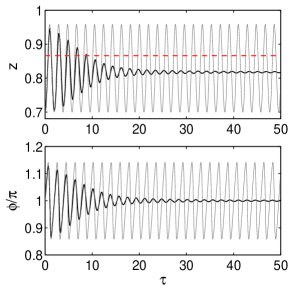
Figure 6: (Color online) The phase-locked MQST state dynamics: quantum averages (black lines) vs classical dynamics (grey lines). The dashed line in the upper panel gives the classical stationary point $z_{s}=0.866$. Here $N=1000$, $\gamma=2$ (whereas $\gamma_{\textrm{c}}=1.23$) and $\varepsilon=0$. The initial Gaussian distribution of width $\Delta z=0.12$ centered at the point $z_{0}=0.78$ and with phase $\phi=\pi$ was used.

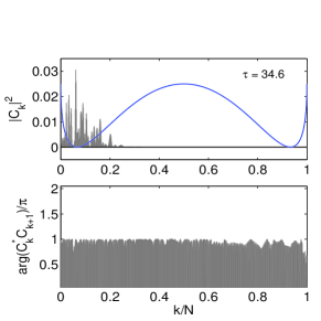
Figure 7: (Color online) The atomic number distribution (a) (represented by vertical bars) of the phase-locked MQST state and the distributed quantum phase (b) (given by bars). The line in panel (a) gives a schematic portrait of the inverse quantum potential $-V_{-}(1-2k/N)$.

To get a quantitative estimate of the validity the classical dynamics, one can use the standard deviations of the quantum variables, defined as $\Delta z=2\Delta x=2||x-\langle x\rangle||=\left[\langle(x-\langle x\rangle)^{2}\rangle\right]^{\frac{1}{2}}$ and

$$\Delta e^{i\hat{p}} = ||e^{i\hat{p}}-\langle e^{i\hat{p}}\rangle||$$ (47)

$$= \left[\langle\left(e^{-i\hat{p}}-\langle e^{-i\hat{p}}\rangle\right)\left(e^{i\hat{p}}-\langle e^{i\hat{p}}\rangle\right)\rangle\right]^{\frac{1}{2}}$$

$$= \left[1-|\langle e^{i\hat{p}}\rangle|^{2}\right]^{\frac{1}{2}}$$

(we assume that $|\langle N,0|\Psi\rangle|=0$, in the case of $|\langle N,0|\Psi\rangle|\neq 0$ and $|\langle 0,N|\Psi\rangle|=0$ one can use the operator $e^{-i\hat{p}}$ instead with similar result). From Eq. (47) one concludes that for the average phase defined in Eq. (46) we have $\langle e^{i\hat{p}}\rangle=\alpha e^{i\langle\phi\rangle}$ with some $\alpha\leq 1$. The quantum dispersions satisfy the uncertainty relation

$$\frac{\Delta e^{i\hat{p}}}{|\langle e^{i\hat{p}}\rangle|}\Delta z\geq h.$$ (48)

For the simulations presented in figure 6, the standard deviation $\Delta z$ decreases from $0.122$ settling to $0.096$ while $\Delta e^{i\hat{p}}$ grows from $0.0479$ to $0.268$ (the average $|\langle e^{i\hat{p}}\rangle|$ decreases from $0.999$ to $0.963$). In this case the l.h.s. in the inequality (48) grows in the result of evolution by less than one order of magnitude as compared to the initial value on the order of the r.h.s..

It was the running phase MQST which was observed in the experiment of Ref. TunTrap . The classical dynamics of the running phase MQST is well understood MFDW . We have found that the quantum correction to the classical running phase is in the form of the quantum collapses and revivals, see Figs. 8 and 9. Though we show the numerical simulations for small number of atoms $N=200$, the time of occurrence of the first collapse of the running phase does not seem to depend on the number of atoms but on the initial conditions, for instance the phase (the subsequent quantum revivals and collapses do depend on $N$: we have found no revivals for $N=1000$ up to $\tau=200$). This effect can be observed in an experiment if the dynamics is followed for longer times.

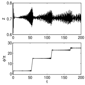
Figure 8: The quantum collapses and revivals of the running phase MQST state. We use $N=200$, $\gamma=5$, $\varepsilon=0$. The initial condition is a Gaussian with the average $z_{0}=0.91$ (the $y$-axis is cut below the upper limit of $z$ for better visibility of the dynamics at large times), $\phi(0)=0$ (thus $\gamma_{\mathrm{c}}=3.35$) and the Gaussian width $\sigma=0.1N$.

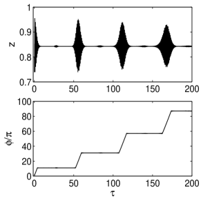
Figure 9: The same as in Fig 8 ($N=200$, $\gamma=5$, $\varepsilon=0$) for the Gaussian initial condition with the average $z_{0}=0.8$ and the initial phase $\phi(0)=0.75\pi$ (thus $\gamma_{\mathrm{c}}=1.8$) and width $\sigma=0.05N$.

For $\phi(0)=0$ the first collapse of the running phase occurs about the value $\phi(\tau)=3\pi$, which is close to final value of the phase in the experiment of Ref. TunTrap on the MQST (this depends on the initial conditions: for $\phi(0)=0.75\pi$ the first collapse occurs at $\phi(\tau)\approx 11\pi$, see Fig. 11). The growth of the quantum average $\langle\phi\rangle$ is interrupted by plateaus of constant phase, while the classical phase follows the linear growth, see Figs. 10 and 11. In the case of $\phi(0)=0.75\pi$, Figs. 9 and 11, the initial state is more classical, i.e. the corresponding uncertainty relation (48) is approximately equality at $t=0$ (whereas in the case of $\phi=0$, initially, the l.h.s of Eq. (48) is larger than the r.h.s. by an order of magnitude).

Our principal result is that the first quantum collapse is associated with an exponential growth of quantum fluctuations of the phase distribution, see Figs. 12 and 13, which reach a maximal value at the first occurrence of the quantum collapse. In this case, the l.h.s. of the inequality (48) grows by more than two orders of magnitude reaching the value of order one at the first collapse (the average $|\langle e^{i\hat{p}}\rangle|$ decreases from $0.97$ to $0.03$). The growing fluctuations are also seen in the experimental results on the running phase MQST presented in Ref. TunTrap .

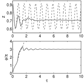
Figure 10: The classical dynamics (thick dashed lines) and the corresponding quantum averages (thin solid lines) at the first occurrence of quantum collapse of the running phase MQST state of Fig. 8.

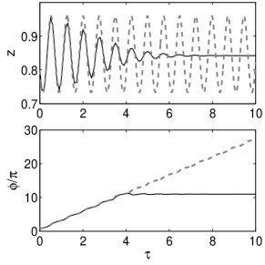
Figure 11: The same as in Fig. 10 but for $\phi(0)=0.75\pi$, i.e. corresponding to Fig. 9.

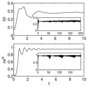
Figure 12: The dispersions of the quantum distributions of $z$ and $e^{i\hat{p}}$ corresponding to Figs. 8 and 10. The insets show the full picture of time dependence of the dispersions.

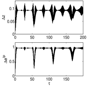
Figure 13: The dispersions of the quantum distributions of $z$ and $e^{i\hat{p}}$ corresponding to Figs. 9 and 11.

Finally, we note that the running phase MQST can be described by the WKB approach by setting in Eq. (12) $\phi=\phi(\tau)$ (i.e. the classical solution) and solving the time-dependent Schrödinger equation analogous of Eq. (15). In this approach, it is the running classical phase what makes the potential (16), seen by the effective quantum particle, asymmetric in $x$, since now we have $\mathcal{V}_{MQST}=\mathcal{V}_{0}(x,\phi)+\dot{\phi}x$. This gives an elementary explanation why BEC is trapped in one well of the double-well trap.

VII Conclusion

We have proposed an analytical approach for description of quantum phenomena in the system of large number of interacting identical bosons occupying only few modes (two in the present study). The method links the many-boson system with the dynamics of a single quantum particle in a potential, where the normalized occupation numbers of the different modes in the Fock space serve as the particle co-ordinates. We have used as the example the well-known two-mode model, describing, for instance, BEC tunneling in a double-well trap, i.e. the boson Josephson effect. The method allowed to account for the mean-field stationary points and their stability, trace analytically the transformation of the ground state of the system of identical bosons in both attractive and repulsive case, derive the quantum fluctuations of the number of atoms in the ground state, relate the appearance of the macroscopic quantum self-trapping phenomenon to the double-well shape of the potential for the effective quantum particle and give a quantum explanation of the phase-locked and running phase self-trapped states of BEC in the double-well trap. We also predict a new phenomenon – quantum collapses and revivals of classical running phase of the macroscopic quantum self-trapped state.

Our method awaits other important applications, where few-mode boson models naturally appear, including the theory of molecular-atomic coherence in BEC AMTheory , the quantum model of nonlinear intraband tunneling of BEC in optical lattices SK2 ; SK3 and many others.

Appendix A The full two-mode boson-Josephson model

One can show that the full two-mode boson model describing BEC in a double-well trap can be cast in the (dimensional) form

$$H = \delta Va_{1}^{\dagger}a_{1}-[J_{\mathrm{lin}}+J_{\mathrm{nonl}}(N-1)](a_{1}^{\dagger}a_{2}+a_{2}^{\dagger}a_{1})$$

$$+ \frac{\rho_{1}-\rho_{2}}{2}\left[(a^{\dagger}_{1}a_{1})^{2}+(a^{\dagger}_{2}a_{2})^{2}\right]+\frac{\rho_{2}}{2}\left(a_{1}^{\dagger}a_{2}+a_{2}^{\dagger}a_{1}\right)^{2},$$

where some scalar $N$-dependent term has been discarded. The coefficients are given as $J_{\mathrm{lin}}=\delta E/2$,

$$J_{\mathrm{nonl}}=-g\int\mathrm{d}^{3}\,{\bf x}\varphi_{\alpha}({\bf x})\varphi_{\beta}^{3}({\bf x}),$$

$$\rho_{1}=g\int\mathrm{d}^{3}{\bf x}\,\varphi_{\alpha}^{4}({\bf x}),$$

$$\rho_{2}=g\int\mathrm{d}^{3}\,{\bf x}\varphi_{\alpha}^{2}({\bf x})\varphi_{\beta}^{2}({\bf x})$$ (50)

(the subscripts $\alpha$ and $\beta$ are permutation of the list $\{L,R\}$ and the functions give the localized states in the left or right well defined by the appropriate linear combinations of the ground state and the first exited state, see section II). The derivation is similar to that of Refs. AB ; GO and is omitted. However, with the help of numerical evaluation, one can verify that for all double-well traps with two lower degenerate levels $E_{1}$ and $E_{2}$ satisfying the inequality $\delta E=E_{2}-E_{1}\ll E_{3}-E_{2}$ the coefficients satisfy

$$\rho_{1}\gg\rho_{2}\gg|J_{\mathrm{nonl}}|.$$ (51)

The coefficients $J_{\mathrm{lin}}$ and $J_{\mathrm{nonl}}(N-1)$, however, can be of the same order. Discarding the small terms and dividing the Hamiltonian by the quantity $[J_{\mathrm{lin}}+J_{\mathrm{nonl}}(N-1)]N$ one gets the reduced model given by Eq. (1) with a different definition of the parameters.

Appendix B Proof that the local minimum of $-V_{-}(z)$ at the negative $z$ is the absolute minimum

Denote $z_{-}$ and $z_{+}$ the negative and positive local minima of $-V_{-}(z)$ for $\gamma>\gamma_{\mathrm{cr}}$. Using $\varepsilon z=z^{2}(\gamma-(1-z^{2})^{-1/2})$ from Eq. (21) into the expression for the quantum potential (19) we get

$$V_{-}(z_{\pm})=\frac{z_{\pm}^{2}}{2}\left(\frac{2}{\sqrt{1-z_{\pm}^{2}}}-\gamma\right)+\sqrt{1-z_{\pm}^{2}}.$$ (52)

Using Eq. (21) again to obtain $(1-z_{-}^{2})^{-1/2}\geq\gamma$ and $(1-z_{+}^{2})^{-1/2}\leq\gamma$, we arrive at the estimates

$$V_{-}(z_{+})\leq\frac{1-z_{-}^{2}/2}{\sqrt{1-z_{-}^{2}}},\quad V_{-}(z_{-})\geq\frac{1-z_{-}^{2}/2}{\sqrt{1-z_{-}^{2}}},$$ (53)

where the equality sign is for $\varepsilon=0$. Now, since the function $f(z)\equiv(1-z^{2}/2)/\sqrt{1-z^{2}}$ is monotonously growing for $0<z<1$, one needs to compare just the values $|z_{-}|$ and $z_{+}$. But it is evident from Fig. 1(b) that $z_{+}\leq|z_{-}|$ (the equality for $\varepsilon=0$) which leads to $V_{-}(z_{-})\geq V_{-}(z_{+})$. Indeed, $z_{\pm}$ are the intersections of the curve $\mathrm{lhs}(z)\equiv\gamma-(1-z^{2})^{-1/2}$ with the two branches of $\varepsilon/(2z)$, while its intersections $z^{(\pm)}_{0}$ with the $z$-axis are equal in the absolute value. But, since the derivative of $\mathrm{lhs}(z)$ has the sign opposite that of $z$, we get $z_{-}<z_{0}^{(-)}$ and $z_{+}<z_{0}^{(+)}$ what completes the proof.

Appendix C The details of the analysis of the ground state of BEC

To find the ground state of large BEC ($N\gg 1$) one needs to compare just the zero-point energies at the extremal points (which is the classical energy of the stationary point, Eqs. (24) and (25)). Using Eq. (21) we get

$$V_{\pm}(z_{\pm})=-\frac{\gamma z_{\pm}^{2}}{2}\mp\frac{1}{\sqrt{1-z_{\pm}^{2}}},$$ (54)

where $z_{\pm}=z_{s}^{(\pm)}$ is the corresponding extremal point of $V_{\pm}(z)$.

Consider the symmetric case $\varepsilon=0$ and a repulsive BEC $\gamma>0$. The extremal points are $z_{+}=0$ and $z_{-}=0$ for $\gamma<\gamma_{\mathrm{cr}}=1$, while $z^{2}_{-}=1-\gamma^{-2}$ otherwise. Using them into Eq. (54) we get

$$V^{(\mathrm{rep})}_{+}(z_{+})=-1,\quad V^{(\mathrm{rep})}_{-}(z_{-})=\left\{\begin{array}[]{c}1,\;\gamma\leq 1\\ \frac{1+\gamma^{2}}{2\gamma},\;\gamma>1\end{array}\right.$$ (55)

Thus the ground state of a repulsive BEC in the double-well trap is given by the equal distribution of atoms between the wells with the zero phase difference.

On the other hand, for an attractive BEC in a symmetric double-well trap, using Eq. (54) we obtain $z_{-}=0$ and $z_{+}=0$ for $|\gamma|\leq 1$, while $z^{2}_{+}=1-\gamma^{-2}$ otherwise. Eq. (54) then gives

$$V^{(\mathrm{attr})}_{+}(z_{+})=\left\{\begin{array}[]{c}-1,\;|\gamma|\leq 1\\ \frac{1+\gamma^{2}}{2\gamma},\;|\gamma|>1\end{array}\right.,\quad V^{(\mathrm{attr})}_{-}(z_{-})=1,$$ (56)

where now $\gamma<0$. Thus the ground state of an attractive BEC also has equal distribution of atoms between the wells of the double-well trap (with zero phase difference) for $|\gamma|<1$. On the other hand, the ground state of an attractive BEC for $|\gamma|>1$, when there are two local bound states (in the classical case $z_{s}>0$ and $z_{s}<0$) corresponding to unequal distributions, is given by the ground state $\psi(z)$ of the effective particle in the double-well trap $V_{+}(z)$, see Eq. (18). In this case, the classical stationary points feature the spontaneous symmetry breaking.

Finally, since for arbitrary $\varepsilon>0$ the only change is in the position of $z_{\pm}$ and Eq. (54) is derived for arbitrary $\varepsilon$, the ground state of BEC for $\varepsilon\neq 0$ is given by the ground state of Eq. (17) with positive mass. Indeed, we estimate from Eq. (54) using (21):

$$V_{+}(z_{+})<-\frac{z_{+}^{2}}{2}\left(\gamma+\frac{1}{\sqrt{1-z_{+}^{2}}}\right)=-\frac{\varepsilon z_{+}}{4},$$

$$V_{-}(z_{-})>\frac{z_{-}^{2}}{2}\left(\gamma+\frac{1}{\sqrt{1-z_{-}^{2}}}\right)=-\frac{\varepsilon z_{-}}{4}.$$ (57)

We arrive at the needed inequality $V_{+}(z_{+})<V_{-}(z_{-})$ for all $\varepsilon$, since for a repulsive BEC the absolute minimum of $-V_{-}(z)$ is negative $z_{-}<0$ (see Fig. 1(a)) while $z_{+}>0$ Eq. (21). On the other hand, by Eqs. (21) and (20), for an attractive BEC $z_{+}$ is the absolute minimum of the double well $V_{+}(z)$ (see Fig 1(a)) and is positive, while $z_{-}$ is negative.

Appendix D The relative atom number fluctuations in the positive mass case

We have $\langle(x-x_{s})^{2}\rangle=\sigma^{2}_{+}/2$, where

$$\sigma^{2}_{+}=\frac{1}{2N}\left[\frac{(1-z_{s})^{1/2}}{\gamma+(1-z_{s}^{2})^{-3/2}}\right]^{1/2}.$$ (58)

From Eq. (21) for positive mass case we get $(1-z_{s}^{2})^{1/2}=\frac{\varepsilon}{2z_{s}}-\gamma$. Now using Eq. (29) we obtain:

$$\frac{\varepsilon}{2z_{s}}-\gamma=1+\frac{\varepsilon^{2}}{8(1+\gamma)^{2}}+O(\varepsilon^{4}),$$

$$\gamma+\left(\frac{\varepsilon}{2z_{s}}-\gamma\right)^{3}=(1+\gamma)\left[1+\frac{3\varepsilon^{2}}{8(1+\gamma)^{3}}+O(\varepsilon^{4})\right].$$

Therefore

$$\sigma^{2}_{+}=\frac{1}{2N}(1+\gamma)^{-1/2}\left[1-\frac{\varepsilon^{2}(4+\gamma)}{16(1+\gamma)^{3}}+O(\varepsilon^{4})\right].$$ (59)

References

- (1) N.N. Bogoliubov, N.N. Bogoliubov Jr., Introduction to Quantum Statistical Mechanics (World Scientific, Singapore, 1982).
- (2) L. P. Pitaevskii and S. Stringari, Bose-Einstein Condensates in Gases (Cambridge University Press, Cambridge, England, 2003).
- (3) Y. Castin and R. Dum, Phys. Rev. A 57, 3008 (1998).
- (4) S. Aubry, S. Flach, K. Kladko, and E. Olbrich, Phys. Rev. Lett. 76, 1607 (1996).
- (5) G. J. Milburn, J. Corney, E. M. Wright and D. F. Walls, Phys. Rev. A 55, 4318 (1997).
- (6) A. Vardi and J. R. Anglin, Phys. Rev. Lett. 86, 568 (2001).
- (7) J. R. Anglin and A. Vardi, Phys. Rev. A 64, 013605 (2001).
- (8) K. W. Mahmud, H. Perry, and W. P. Reinhardt, Phys. Rev. A 71, 023615 (2005).
- (9) V. S. Shchesnovich and V. V. Konotop, Phys. Rev. A 75, 063628 (2007).
- (10) V. S. Shchesnovich and V. V. Konotop, Phys. Rev. A 77, 013614 (2008).
- (11) S. Mossmann and C. Jung, Phys. Rev. A 74, 033601 (2006).
- (12) E. J. Mueller, T-L. Ho, M. Ueda, and G. Baym, Phys. Rev. A 74, 033612 (2006).
- (13) Y. Zhou, H. Zhai, R. Lü, Zh. Xu, and L. Chang, Phys. Rev. A 67, 043606 (2003).
- (14) T.-L. Ho and C. V. Ciobanu, J. Low. Temp. Phys. 125, 257 (2004).
- (15) P. A. Braun, Rev. Mod. Phys. 65, 115 (1993).
- (16) E. M. Graefe and H. J. Korsch, Phys. Rev. A 76, 032116 (2007).
- (17) A. J. Leggett, Rev. Mod. Phys. 73, 307 (2001).
- (18) R. Gati and M. K. Oberthaler, J. Phys. B: At. Mol. Opt. Phys. 40, R61 (2007).
- (19) M. Albiez, R. Gati, J. Fölling, S. Hunsmann, M. Cristiani, and M. K. Oberthaler, Phys. Rev. Lett. 95, 010402 (2005).
- (20) Y. Shin, M. Saba, T. A. Pasquini, W. Ketterle, D. E. Pritchard, and A. E. Leanhardt, Phys. Rev. Lett. 92, 050405 (2004).
- (21) C. Lee, Phys. Rev. Lett. 97, 150402 (2006).
- (22) M. Jääskeläinen and P. Meystre, Phys. Rev. A 73, 013602 (2006).
- (23) B. V. Hall, S. Whitlock, R. Anderson, P. Hannaford, and A. I. Sidorov, Phys. Rev. Lett. 98, 030402 (2007).
- (24) G.-B. Jo, Y. Shin, S. Will, T. A. Pasquini, M. Saba, W. Ketterle, D. E. Pritchard, M. Vengalattore and M. Prentiss, Phys. Rev. Lett. 98, 030407 (2007).
- (25) D. Ananikian and T. Bergeman, Phys. Rev. A 73, 013604 (2006).
- (26) V. S. Shchesnovich, S. B. Cavalcanti and R. A. Kraenkel, Phys. Rev. A 69, 033609 (2004).
- (27) A. Smerzi, S. Fantoni, S. Giovanazzi, and S. R. Shenoy, Phys. Rev. Lett. 79, 4950 (1997); S. Raghavan, A. Smerzi, S. Fantoni, and S. R. Shenoy, Phys. Rev. A 59 620 (1999).
- (28) L. Bernstein, J. C. Eilbeck and A. C. Scott, Nonlinearity 3, 293 (1990).
- (29) R. Gati, J. Esteve, B. Hemmerling, T. B. Ottenstein, J. Appmeier, A. Weller and M. K. Oberthaler, New J. Phys. 8, 189 (2006).
- (30) A. N. Salgueiro, A. F. R. de Toledo Piza, G. B. Lemos, R. Drumond, M. C. Nemes, and M. Weidemüller, Eur. Phys. J. D 44, 537 (2007).
- (31) S. Raghavan, A. Smerzi and V. M. Kenkre, Phys. Rev. A 60, R1787 (1999).
- (32) H. Tal-Ezer and R. Kosloff, J. Chem. Phys. 81, 3967 (1984).
- (33) L. Susskind and J. Glogower, Physics (Long Island City, N.Y.) 1, 49 (1964).
- (34) M. Kostrun, M. Mackie, R. Côté, and J. Javanainen, Phys. Rev. A 62, 063616 (2000); J. Calsamiglia, M. Mackie, and K.-A. Suominen, Phys. Rev. Lett. 87, 160403 (2001) .