Quasicondensation and coherence in the quasi-two-dimensional trapped Bose gas

Abstract

We simulate a trapped quasi-two-dimensional Bose gas using a classical field method. To interpret our results we identify the uniform Berezinskii-Kosterlitz-Thouless (BKT) temperature $T_{BKT}$ as where the system phase space density satisfies a critical value. We observe that density fluctuations are suppressed in the system well above $T_{BKT}$ when a quasi-condensate forms as the first occurrence of degeneracy. At lower temperatures, but still above $T_{BKT}$, we observe the development of appreciable coherence as a prominent finite-size effect, which manifests as bimodality in the momentum distribution of the system. At $T_{BKT}$ algebraic decay of off-diagonal correlations occurs near the trap center with an exponent of $0.25$, as expected for the uniform system. Our results characterize the low temperature phase diagram for a trapped quasi-2D Bose gas and are consistent with observations made in recent experiments.

I Introduction

The physics of two-dimensional systems is very different from what we observe in the three-dimensional world. The Mermin-Wagner-Hohenberg theorem Mermin and Wagner (1966); Hohenberg (1967) states that thermal fluctuations destroy the long-range order, characteristic of most phase transitions, in systems of reduced dimension. However, in systems that support topological defects, such as vortices, the existence of a quasi-long-range ordered (quasi-coherent) state was predicted to occur by Berezinskii, Kosterlitz and Thouless (BKT) Berezinskii (1971); Kosterlitz and Thouless (1973). The BKT superfluid transition has been experimentally observed in liquid helium thin films Bishop and Reppy (1978), superconducting Josephson-junction arrays Resnick et al. (1981) and in spin-polarized atomic hydrogen Safonov et al. (1998). More recently evidence for the BKT transition in a dilute gas of ⁸⁷Rb atoms was reported by the ENS group Stock et al. (2005); Hadzibabic et al. (2006); Krüger et al. (2007). However, strong fluctuations, the interplay of harmonic confinement and interactions, and finite size effects have made predictions for the low temperature phase diagram of this system the subject of much debate Popov (1983); Petrov et al. (2000); Andersen et al. (2002); Gies et al. (2004); Trombettoni et al. (2005); Simula et al. (2006). Meanfield methods are inapplicable and reliable predictions have only recently become available from classical field and Quantum Monte Carlo methods Simula and Blakie (2006); Holzmann and Krauth (2008).

Limited theoretical understanding has meant that the relationships between bimodality in the density distribution Krüger et al. (2007), algebraic decay of phase coherence Hadzibabic et al. (2006), and thermal activation of phase defects Stock et al. (2005); Hadzibabic et al. (2006) has been unclear and the subject of speculation. In particular, a crucial issue currently under debate is whether the critical point identified using bimodality Krüger et al. (2007) is distinct from the BKT cross-over found in Hadzibabic et al. (2006). In contrast to the ENS results a recent experiment by the NIST group Cladé et al. (2008) suggests that bimodality occurs at higher temperature (i.e. at lower phase space density) than the onset of the BKT superfluid. In this paper we perform a detailed analysis of the low temperature properties of a quasi-2D system to explore this issue. Our results support the NIST observations and show that bimodality occurs at temperatures above the uniform condition for the BKT transition Prokof’ev et al. (2001); Prokof’ev and Svistunov (2002). We also show measurable signatures of the degenerate components of the system: quasi-condensate (suppressed density fluctuations), bimodality (coherence), and superfluidity (algebraic decay of correlations).

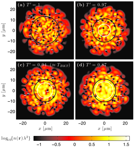
Figure 1: (color online) Instantaneous planar density of a quasi-2D classical field at a range of temperatures. Inner white (outer black) circle marks the 1/e-boundary of the condensate (quasi-condensate) density. Vortices (+) and anti-vortices (-) are shown. Results indicated for various values of reduced temperature, $T^{\prime}$ (see Sec. II.4). Other simulation parameters given in the text.

To provide insight into the interplay of these degenerate regimes, Fig. 1 shows four microstates of the quasi-2D trapped gas for a range of temperatures that indicate important features of this system: In all cases a quasi-condensate (as defined below) is present, and is the only degenerate component for the highest temperature result Fig. 1(a). As the temperature decreases [Fig. 1(b)] spatial coherence emerges, marked by a finite condensate density. However, in this temperature regime vortices are prolific and we frequently observe free vortices penetrating the condensate. For the lower temperature results (i.e. $T\lesssim T_{BKT}$) [see Figs. 1(c) and (d)] we see that in the central (condensate) region density fluctuations are significantly reduced and vortices and anti-vortices are mostly found paired (i.e. in close proximity).

II Formalism

Here we consider a harmonically trapped Bose gas described by the Hamiltonian

$$\hat{H}=\int d^{3}x\,\hat{\Psi}^{\dagger}\left\{H_{sp}+\frac{2\pi a\hbar^{2}}{m}\hat{\Psi}^{\dagger}\hat{\Psi}\right\}\hat{\Psi},$$ (1)

where

$$H_{sp}=\frac{p^{2}}{2m}+\frac{1}{2}m(\omega_{x}^{2}x^{2}+\omega_{y}^{2}y^{2}+\omega_{z}^{2}z^{2}),$$ (2)

is the single particle Hamiltonian, $m$ is the atomic mass, and $a$ is the $s$-wave scattering length. For $\omega_{z}\gg\omega_{x},\omega_{y}$ the $z$-axis degree of freedom is frozen out at sufficiently cold temperatures, and the system becomes quasi-2D. The dimensionless 2D coupling constant is $\tilde{g}=\sqrt{8\pi}a/a_{z},$ with $a_{z}=\sqrt{\hbar/m\omega_{z}}$. We will assume that $a_{z}\gg a$ so that the scattering is approximately three-dimensional Petrov et al. (2000), a condition well-satisfied in the ENS and NIST experiments Stock et al. (2005); Hadzibabic et al. (2006); Krüger et al. (2007); Cladé et al. (2008).

In what follows we will take $\mathbf{r}=(x,y)$ to be the 2D position vector, all densities to be areal (i.e. integrated along $z$), and the trap to be radially symmetric with $\omega\equiv\omega_{x}=\omega_{y}$ the radial trap frequency. Our results here are for the case of a quasi-2D system of ⁸⁷Rb atoms with trap frequencies $\omega=2\pi\times 9.4\,$Hz, $\omega_{z}=2\pi\times 1.88\,$kHz and a coupling constant of $\tilde{g}=0.107$. For reference, in ENS experiments $\tilde{g}\approx 0.13$ Hadzibabic et al. (2006), whereas in the NIST experiments $\tilde{g}\approx$0.02 Cladé et al. (2008).

Our simulation method (see Appendix A) is based upon a classical field (denoted by $\Phi$) representation of the low energy modes of the system. The remaining high energy modes, that we refer to as the above region, are described by a quantum field, $\hat{\psi}$ Blakie and Davis (2005). Averages of the full field, $\hat{\Psi}=\Phi+\hat{\psi}$, are obtained by time-averaging the dynamics of the classical field and ensemble averaging the properties of $\hat{\psi}$ using a Hartree-Fock meanfield analysis Simula and Blakie (2006); Davis and Blakie (2006); Simula et al. (2008). Because the classical field approach captures the non-perturbative dynamics of the low energy modes, it is valid in the critical regime which extends over a large temperature region in the 2D system and was the basis of the definitive analysis of the uniform 2D Bose gas by Prokof’ev et al., in Ref. Prokof’ev et al. (2001). Here our approach provides a good description of the trapped system when: (i) $\tilde{g}$ is small compared to unity; (ii) all modes of the classical field are appreciably occupied; and (iii) the fluctuation region is fully contained within the classical field (see Appendix A). Our approach is computationally efficient and suitable for studying non-equilibrium dynamics, such as the vortex dynamics pictured in Fig. 1.

We now discuss the various ways of characterizing the low temperature components of the quasi-2D system that are useful for interpreting the results of our calculations.

II.1 Superfluid model of Holzmann et al.

Recently Holzmann et al. Holzmann and Krauth (2008) have extended a Quantum Monte Carlo method to study this system and have proposed a model for the superfluid component based on a local density application of the uniform results Prokof’ev et al. (2001); Prokof’ev and Svistunov (2002). In detail, they suggested a superfluid density of the form

$$n_{sf}(r) = \left\{\begin{array}[]{cc}\frac{(m\omega r_{cr})^{2}}{2\hbar^{2}\tilde{g}}\left(1-\frac{r^{2}}{r_{cr}^{2}}\right)+\frac{4}{\lambda^{2}},&\,\,\,\,r\leq r_{cr}\\ 0,&\,\,\,\,r>r_{cr}\end{array}\right.$$ (5)

where $r_{cr}$ is the radius at which the trapped system density equals the (temperature dependent) critical value

$$n_{cr}=\lambda^{-2}\log\left(\frac{C}{\tilde{g}}\right),$$ (6)

with $C=380\pm 3$ and $\lambda=h/\sqrt{2\pi mk_{B}T}$ ($n_{cr}\lambda^{2}$ is the critical phase-space density for the uniform 2D Bose gas to undergo the BKT transition Prokof’ev et al. (2001)). To obtain the superfluid density using (5) hence requires a comprehensive calculation of the system density (e.g. using classical field theory and Quantum Monte Carlo) from which $r_{cr}$ can be determined.

In Holzmann and Krauth (2008) Eq. (5) was shown to provide a reasonable description of the moment of inertia obtained directly from Monte Carlo calculations. However this model has curious behavior at the transition whereby the superfluid density discontinuously emerges as a sharp spike when the central (peak) density of the system exceeds $n_{cr}$. The temperature where this occurs is denoted $T_{BKT}$ Holzmann and Krauth (2008); Holzmann et al. (2008); Bisset et al. (2009).

II.2 Quasi-condensate

Quasi-condensate is the component of the system with suppressed density fluctuations, defined by Prokof’ev et al. (2001)

$$n_{qc}(\mathbf{r})=\sqrt{2\langle\hat{n}(\mathbf{r})\rangle^{2}-\langle\hat{n}(\mathbf{r})^{2}\rangle},$$ (7)

where $\hat{n}(\mathbf{r})=\hat{\Psi}^{\dagger}(\mathbf{r})\hat{\Psi}(\mathbf{r})$ is the density operator for the system. Note, that for a normal system with Gaussian density fluctuations $\langle\hat{n}(\mathbf{r})^{2}\rangle=2\langle\hat{n}(\mathbf{r})\rangle^{2}$ so that $n_{qc}=0$. Definition (7) was shown to furnish a universal quantity in the uniform gas Prokof’ev et al. (2001).

II.3 Coherence

There are many ways to define coherence, especially so for an inhomogeneous system, and here we choose to use a measure based on the Penrose-Onsager criterion. Normally this criterion is that a single a macroscopic eigenvalue of the one-body density matrix

$$G(\mathbf{r},\mathbf{r}^{\prime})=\langle\hat{\Psi}^{\dagger}(\mathbf{r})\hat{\Psi}(\mathbf{r}^{\prime})\rangle,$$ (8)

is equivalent to the condensate number, with respective eigenfunction characterizing the condensate mode. Formally, this analysis is only valid in the thermodynamic limit, and finite size effects make the unique identification of condensate rather fraught – especially so in the 2D case. Here we choose to use the largest eigenvalue and eigenvector as a measure of coherence, and refer to them as condensate only for clarity Penrose and Onsager (1956); Blakie and Davis (2005). We denote the condensate density as $n_{c}(\mathbf{r})$, which provides a spatial characterization of the system coherence (e.g. the condensate mode boundary shown in Fig. 1).

Figure 2: (color online) Component densities along the $x$-axis at (a) $T^{\prime}=0.91$ and (b) $T^{\prime}=1.0$ : Total density $n(x)$ (dotted-line), quasi-condensate $n_{qc}(x)$ (dashed), condensate $n_{c}(x)$ (solid) and superfluid $n_{sf}(x)$ (shaded region). (c) Fraction of atoms in quasi-condensate (dots), condensate (squares) and superfluid (triangles). System (a): $T=30.6\,$nK and $N=9.9\times 10^{3}$, system (b): $T=48.5\,$nK and $N=25.9\times 10^{3}$. Other parameters as discussed in the text.

II.4 Reduced temperature

The classical field approach we employ uses a fixed classical region with its total energy as the macroscopic control parameter. As we vary this parameter both the temperature and number of particles vary (see Appendix A). To remove leading order effects of varying $N$ we scale all temperatures according to $T^{\prime}=T/T_{0}$, where $T_{0}$ is the quasi-2D ideal gas BEC temperature. We numerically calculate $T_{0}$ by determining the saturated thermal cloud occupation according to

$$N(T)=\sum_{j\neq 0}\left(e^{(\epsilon_{j}-\epsilon_{0})/k_{B}T}-1\right)^{-1},$$ (9)

where $\{\epsilon_{j}\}$ are the 3D harmonic oscillator energies for our trap. Inverting this relation numerically we obtain $T_{0}(N)$ - i.e. the temperature at which the thermal cloud of $N$ atoms is saturated. The inclusion of quasi-2D effects, i.e. excited $z$-states, is typically important, producing an appreciably lower critical temperature than the pure 2D prediction $T_{2D}=\sqrt{6N\omega_{x}\omega_{z}}\hbar/\pi k_{B}$ Bagnato and Kleppner (1991).

III Results

III.1 Components of the quasi-2D trapped gas

Time-averaged density profiles are shown in Figs. 2(a) and 2(b) for a system with $\tilde{g}=0.107$. Figure 2(a) shows the system density when both quasi-condensate and condensate components are present, whereas Fig. 2(b) shows the density at a higher temperature where only a quasi-condensate component exists. Figure 2(c) plots the degenerate components of the system over a large temperature range. At the highest temperatures we observe a small quasi-condensate fraction, which increases with decreasing temperature. Below $T^{\prime}\approx 0.98$ the condensate fraction becomes appreciable (indicated as the coherence temperature $T_{coh}$ in Fig. 2(c)). In this regime we commonly see free vortices in the condensate [e.g. see Fig. 1(b)] which have a profound effect on its coherence properties. Finally, at $T_{BKT}$ ($T^{\prime}\approx 0.93$) the peak density at the trap center satisfies Eq. (6) and the model, Eq. (5), predicts a non-zero superfluid fraction. Here we observe the occurrence of vortices in the condensate to be much less frequent than at higher temperatures, and those found are usually paired [e.g. see Fig. 1(c–d)]. As the temperature decreases further, the relative difference between quasi-condensate, condensate and superfluid fractions decreases, though they are always clearly distinguishable.

An important result of this paper is that the emergence of coherence occurs at higher temperatures than that where the conditions for uniform system superfluidity are satisfied, $T_{BKT}$, i.e. the emergence of spatial coherence in the trapped system occurs before the peak phase space density satisfies Eq. (6). We have carried out simulations for $\tilde{g}$ values in the range of $0.02$–$0.107$ and observed similar results.

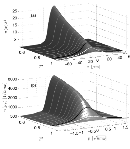
Figure 3: Density distributions versus temperature. (a) Position phase-space density and (b) momentum space density distributions. The black (white) curves mark the densities at $T_{BKT}$ ($T_{coh}$) [also see Fig. 2]. Parameters as in Fig. 2

In Fig. 3 we show the position and momentum density distributions for our system as a function of temperature. In Fig. 3(a) the position dependent phase-space density is seen to smoothly peak as the temperature decreases FN1 . We have confirmed that at low temperatures the central density is well-described by a Thomas-Fermi-type profile of the form $n(r)\sim n(0)-m^{2}\omega^{2}r^{2}/2\hbar^{2}\tilde{g}$ (also see Holzmann and Krauth (2008)). Additionally, we observe that whenever appreciable quasi-condensate is present the density profile bulges slightly (e.g. see Fig. 2(b)). Figure 3(b) shows that for temperatures below $T^{\prime}\approx 0.98$ (where coherence is observed) that a strong bimodality is apparent in the momentum space density of the system associated with the extended spatial coherence arising from the condensate. (Note that the momentum density is shown on a logarithmic scale so that the change from the flat profile at $T^{\prime}\approx 1$ is quite profound). We emphasize that this bimodality is clearly apparent at temperatures well-above $T_{BKT}$.

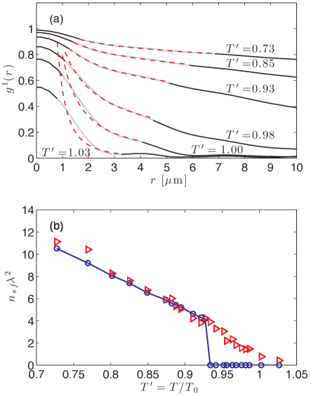
Figure 4: (color online) (a) $g^{1}(r)$ for various temperatures (solid lines). Fitting region (light colored segments of curves) and algebraic fits (dashed) are also shown. (b) Peak superfluid density determined from fits to algebraic decay (triangles) and from model density, Eq. (5) (circles). Parameters as in Fig. 2

III.2 Decay of coherence

An important prediction of the BKT theory for the uniform system is that in the superfluid regime off-diagonal correlations (phase coherence) decay algebraically, i.e. $G(r)\sim r^{-\alpha},$ where $r$ is the spatial separation and the exponent relates to the superfluid density as $\alpha=1/n_{sf}\lambda^{2}$. At $T_{BKT}$ the superfluid transition occurs with $n_{sf}\lambda^{2}=4$ (i.e. $\alpha=0.25$) Kosterlitz and Thouless (1973) and at temperatures above $T_{BKT}$ the system is normal with exponentially decaying correlations.

Here we investigate the nature of off-diagonal correlations in the trapped system Bezett et al. (2008). Because of spatial inhomogeneity the first order correlation function depends on centre-of-mass and relative coordinates, and we therefore choose to examine these correlations symmetrically about the trap center. The normalized correlation function we evaluate is FN2

$$g^{1}(\mathbf{r}) = \frac{\left\langle\Phi^{*}(\mathbf{r}/2)\Phi(-\mathbf{r}/2)\right\rangle}{\sqrt{\langle\hat{n}(\mathbf{r}/2)\rangle\langle\hat{n}(-\mathbf{r}/2)\rangle}},$$ (10)

and typical results for a range of temperatures are shown in Fig. 4(a). We least-squares fit a model decay curve of the form $g^{1}(r)\propto 1/r^{\alpha}$ over the spatial range $1.2\lambda<r<5\lambda$ to determine the exponent $\alpha$. The lower spatial limit excludes the short range contribution of normal-component atoms, while the upper limit restricts the effects of spatial inhomogeneity (typical size of cloud is of order $30\lambda$). The model fits in Fig. 4(a) are poor in the three highest temperature cases, suggesting that the algebraic fit is inappropriate. Using the fitted values of $\alpha$ we infer the superfluid density at the trap center according to $n_{sf}(0)=1/\alpha\lambda^{2}$. The results, shown in Fig. 4(b), compare well with the peak of the model superfluid density, Eq. (5), for temperatures below $T_{BKT}$ ($T^{\prime}\approx 0.93$). At higher temperatures (where $n(0)<n_{cr}$) the two results disagree, however in this temperature range the algebraic fit is poor and an exponential fit to $g^{1}(r)$ appears to be more appropriate.

These results can provide us with an indication that our identification of the superfluid transition is consistent: Using $\alpha=0.25$ as the condition for identifying the BKT transition and comparing to our numerical fits for $\alpha$ would suggest that $T_{BKT}=(0.89-0.94)T_{0}$, consistent with $T_{BKT}$ as identified according to condition (6).

III.3 Relation to experiments

Our results can be compared against the recent experiments at ENS and NIST. Krüger et al. Krüger et al. (2007) (ENS) determined the “exact critical point” by observing bimodality in the density distribution after expansion. Those results suggested that the occurrence of bimodality coincided with the emergence of superfluidity in the system. However, Cladé et al. Cladé et al. (2008) (NIST), instead saw bimodality occurring prior to the superfluid transition. It is difficult to directly compare each experiment as they differ in several aspects: the ENS experiment typically involved several 2D systems and a large $\tilde{g}$ value, whereas the NIST experiment isolated a single 2D system with a smaller $\tilde{g}$ value. Our results are for a $\tilde{g}$ value intermediate to both experiments, but suggest that bimodality is distinct from superfluidity. However, as the relative temperature separation between these phenomena is quite small they may be difficult to distinguish in practice if temperature resolution is poor. We also note that the ENS experimental procedure was to release the gas for $22\,$ms of time-of-flight before absorption imaging of the system density. This time scale is on the order of the characteristic time for expansion in the weak trap direction ($\omega_{x}\approx 2\pi\times 9.4\,$Hz). Thus the measured density distribution along $x$ is in an intermediate regime not well-represented by the in situ spatial or momentum densities, but is in some sense a convolution of the features of both. A semiclassical analysis of this expansion is presented in Hadzibabic et al. (2008). While the quasi-condensate exhibits a certain amount of spatial bulging, our conjecture is that the sharp bimodal feature seen in the experiment (Fig. 2 of Krüger et al. (2007)) is almost certainly due to the onset of coherence [see Fig. 3(b)]. This could be verified experimentally using longer expansion times to more clearly reveal the system momentum distribution.

In an earlier experiment Hadzibabic et al. (2006) the BKT transition was identified by using a heterodyning scheme to determine when off-diagonal correlations in the central region of the system had an algebraic decay coefficient of $\alpha\approx 0.25$. Our results in Fig. 4 show that $\alpha=0.25$ occurs where the peak density satisfies Eq. (6), which we have used to define $T_{BKT}$. The NIST group has developed a more precise procedure for measuring spatial coherence Cladé et al. (2008), which should allow a more systematic investigation of correlations and their relationship to superfluidity and bimodality.

Another issue of concern has been the difference in temperature between the ideal gas condensation temperature, $T_{0}$, and the emergence of the degeneracy in the interacting system. In Krüger et al. Krüger et al. (2007) the onset of bimodality was found to occur for atom numbers “…about 5 times higher than predicted by the semiclassical theory of Bose-Einstein condensation (BEC) in the ideal gas”. This roughly corresponds to the degeneracy temperature being half that of the ideal gas prediction. In a subsequent work the method for determining temperature was compared with theoretical calculations and was found to underestimate the true temperature by a factor of 0.6-0.7 Hadzibabic et al. (2008). Although residual effects of the optical lattice potential used in the ENS experiment make computing $T_{0}$ difficult it seems that the temperature at which bimodality is observed is close to $T_{0}$. Recent theoretical work Holzmann et al. (2008) has also suggested that $T_{0}$ and $T_{BKT}$ that are quite similar for the regime of the ENS experiment. Clearly additional work examining the critical temperature over a wide parameter regime will be necessary to fully understand this relationship better.

III.4 Relation to theory of Holzmann and coworkers

Recently Holzmann and coworkers have performed Quantum Monte-Carlo calculations of the quasi-2D trapped gas Holzmann and Krauth (2008). Although our results are for a system in a different parameter regime we find qualitatively the same behavior for physical predictions, e.g. the peak in central density curvature occurring in the transition region (see Fig. 3 of Holzmann and Krauth (2008)) and the appearance and behavior of condensate (see Fig. 4 of Holzmann and Krauth (2008)). The Quantum Monte Carlo results did not analyze the transition region with the resolution we have in this work, and it is possible that the appearance of coherence before superfluidity is also revealed in their results FN3 .

Holzmann and coworkers have also developed a rather elegant meanfield theory for predicting superfluid transition Holzmann et al. (2008). While providing a simple means for finding an approximate value for $T_{BKT}$, several aspects of this theory have been scrutinized in Bisset et al. (2009) and shown to be inconsistent. In particular, the use of (i) the total areal density and (ii) a temperature renormalized interaction strength in Eq. (6) to identify the superfluid transition instead of the ground transverse mode density and the bare (ground transverse mode) interaction strength, respectively. Aspects (i) and (ii) were also used to identify the superfluid transition in the Quantum Monte Carlo results and the aforementioned consistency issues may have contributed additional uncertainty in the transition temperature Holzmann and Krauth (2008). Because the system we consider here is more two-dimensional than that in Holzmann and Krauth (2008) FN4 , the distinction between total and ground transverse mode areal densities is negligible for our results. However, in general the ground transverse mode areal density is the relevant quantity to be used in expression (6) (see Bisset et al. (2009) for additional discussion). Additionally, we note that expression (6) is valid in the thermodynamic limit and it is not clear how large finite-size shifts might be. Clearly there is a need for more theoretical calculations in the transition region to better clarify the relationship between coherence and superfluidity.

IV Conclusions

We have provided a comprehensive analysis of the low-temperature properties of the trapped 2D Bose gas and have elucidated the roles of condensation and quasi-condensation. A model for the superfluid density, and the temperature $T_{BKT}$, was proposed in Holzmann and Krauth (2008), and shown to provide a reasonable description of the system’s moment of inertia. Our results show that in the finite system coherence can emerge at temperatures above $T_{BKT}$. In this regime it is not clear if the system has some finite-size induced superfluidity arising from the condensate, as the central coherent region is often penetrated by vortices [e.g. see Fig. 1(b)] which may act to destroy its superfluidity. These observations appear to be in agreement with the results presented in Cladé et al. (2008), and suggest that the strong fluctuations seen experimentally in the initial bimodal state (for $T>T_{BKT}$) are associated with vortices. Our calculations of the off-diagonal correlations reveal that extended coherence emerges at temperature well-above $T_{BKT}$, coinciding with the appearance of bimodality in the momentum distribution, whereas the field develops algebraically decaying correlations, accurately described by the uniform theory of the superfluid system, at lower temperatures $T\lesssim T_{BKT}$.

As shown in Fig. 1, the classical field microstates describe the creation of vortices and their ensuing dynamics. Future work will clarify the nature of vortex pairing, their typical production rates and lifetime, to better understand their role in the equilibrium state.

Acknowledgments

The authors acknowledge valuable discussions with the ENS and NIST groups. PBB and RNB are supported by NZ-FRST contract NERF-UOOX0703. TPS acknowledges JSPS support. MJD acknowledges the Australian Research Council support.

Appendix A Review of PGPE method and validity conditions

In this work we use the classical field method known as the projected Gross-Pitaevskii equation (PGPE) formalism, as summarized in Refs. Blakie and Davis (2005); Davis and Blakie (2006); Simula et al. (2008); Simula and Blakie (2006); Bezett et al. (2008); Blakie et al. (2008); Bradley et al. (2005); Bezett et al. (2009). In particular, in Refs. Simula and Blakie (2006); Simula et al. (2008) this formalism is developed for application to the quasi-2D trapped Bose gas. We briefly summarise this method here before discussing details and validity conditions of our calculations.

A.1 Use of PGPE for determining equilibrium properties

A randomized classical field state ($\Phi$) of definite energy, given by the functional

$$E[\Phi]=\int d^{3}x\,\left\{\Phi^{*}H_{sp}\Phi+\frac{2\pi a\hbar^{2}}{m}|\Phi|^{4}\right\},$$ (11)

is constructed according to the procedure discussed in Sec. V of Ref. Blakie (2008). This state is then evolved according to the PGPE

$$i\hbar\frac{\partial\Phi}{\partial t}=H_{sp}\Phi+\mathcal{P}\left\{\frac{4\pi a\hbar^{2}}{m}|\Phi|^{2}\Phi\right\},$$ (12)

where the projector, $\mathcal{P}$, limits the occupation of the field to single particle harmonic oscillator modes below a specified (single particle) energy cutoff $\epsilon_{\rm cut}$. The PGPE (12) has been demonstrated to be ergodic so that, after the initial field thermalizes, time averaging can be used to obtain equilibrium quantities such as density profiles Blakie and Davis (2005), correlation functions Blakie and Davis (2005); Bezett et al. (2008); Simula et al. (2008), and the temperature and chemical potential Davis and Morgan (2003); Davis and Blakie (2005).

A.2 Validity conditions

The classical field method provides an accurate description of the low energy component of the quasi-2D trapped Bose gas as long as three conditions can be satisfied (see sections 2 and 3 of Blakie et al. (2008) for further details):

1. That $\tilde{g}$ is small compared to unity: This condition ensures that classical fluctuations dominate quantum fluctuations. This condition is well-satisfied in our calculations ($\tilde{g}=0.107$) and in current experiments (for the ENS group $\tilde{g}\approx 0.13$ Hadzibabic et al. (2006) and for the NIST group $\tilde{g}\approx 0.02$ Cladé et al. (2008)).

2. Appreciably occupied modes: In order to apply the classical field description we require that modes of the classical region are appreciably occupied, i.e. that the least occupied mode of the classical region has a mean occupation ($\bar{n}_{\min}$) of order 1 or greater. In practice we analyze this validity requirement in our simulations by calculating $\bar{n}_{\min}$, taken as the average the occupation of the highest energy single particle state (i.e. states with single particle energy $\epsilon\sim\epsilon_{\rm cut}$) Blakie and Davis (2007).

3. Good basis: The energy cutoff $\epsilon_{\rm cut}$ has to be sufficiently large that the single particle eigenstates provide a good basis for describing the interacting classical region modes. The condition for this requirement is that $\epsilon_{\rm cut}^{\prime}\equiv\epsilon_{\rm cut}-\epsilon_{0}\gtrsim{\hbar^{2}}\tilde{g}n/m$, where $\epsilon_{0}$ is the single particle ground state energy, and $n$ is the average 2D spatial density of the classical field. This requirement also ensures that the fluctuation region (universal long wavelength modes) is contained in the classical region. This condition is also discussed in Ref. Prokof’ev et al. (2001).

A.3 Above cutoff atoms

Having ensured a valid classical region simulation, we can add the remaining low-density high-energy particles using a Hartree-Fock description, as discussed in Ref. Simula et al. (2008). This allows us to calculate the total number of atoms and the total density profile for the full quasi-2D Bose gas. As long as the third condition above is well-satisfied, then these high energy atoms are well-described using meanfield theory Prokof’ev et al. (2001).

Figure 5: Quantities determined from classical field evolution as a function of the classical field energy per particle. (a) Simulation temperature. (b) Average occupation of the least occupied mode. (c) Ratio of interaction energy scale to the energy cutoff.

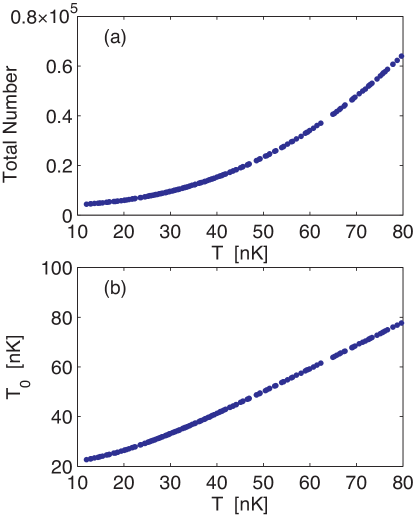
Figure 6: Relevant quantities for our classical field simulations of the quasi-2D trapped Bose gas as a function of temperature. (a) Total particle number of our results and (b) the respective quasi-2D ideal condensation temperature.

A.4 Parameters for calculation

In our calculations we have evolved classical field states with a cut off of $\epsilon_{\rm cut}=125\hbar\omega$, populated with 3750 (classical region) ⁸⁷Rb atoms FN5 for 8.5 seconds (i.e. over 80 radial trap periods). Allowing the first 40 trap periods for rethermalization, we ergodically average using 2000 sampled microstates taken over the last 40 trap periods of evolution.

In Fig. 5 we show various quantities used to establish the validity of our calculations. We choose to keep the classical region size (i.e. $\epsilon_{\rm cut}$) and number of classical region atoms fixed, and vary phase space density of the system by altering the classical region energy as given by Eq. (11). This change in energy directly affects the temperature, which we determine using Rugh’s dynamical definition of temperature (e.g. see Davis and Morgan (2003); Davis and Blakie (2005)), with the results for our parameters shown in Fig. 5(a).

Of the three validity conditions discussed above, only condition (i) can be assured a priori. Conditions (ii) and (iii) need to be verified a posterori as we now discuss. In Fig. 5(b) the average occupation of the least occupied mode is shown. For all calculations this is larger than unity (and near the transition it is typically $\gtrsim 3-4$) so that the classical field approach is well justified for these results. In Fig. 5(c) we show that the ratio $\hbar^{2}\tilde{g}n/m\epsilon_{\rm cut}^{\prime}$ is small, ensuring that our cutoff is large enough to provide a good description of the spectrum and ensuring that the fluctuating region is well contained within the classical field. In summary Figs. 5(b)-(c) show that our method provides an accurate representation of the quasi-2D system we have simulated. In Figs. 6(a)-(b) we show the total atom number [Fig. 6(a)] and associated ideal condensation temperature, $T_{0}$, [Fig. 6(b)], which we use to rescale the temperature. Finally in Fig. 7 we show the thermal activation of the tight degree of freedom as a function of the reduced temperature.

Figure 7: Relative thermal activation of $z$ direction of the system as a function of reduced temperature

References

- Mermin and Wagner (1966) N. D. Mermin and H. Wagner, Phys. Rev. Lett. 17, 1133 (1966).
- Hohenberg (1967) P. C. Hohenberg, Phys. Rev. 158, 383 (1967).
- Berezinskii (1971) V. L. Berezinskii, Sov. Phys. JETP 32, 493 (1971).
- Kosterlitz and Thouless (1973) J. M. Kosterlitz and D. J. Thouless, J. Phys. C: Solid State Physics 6, 1181 (1973).
- Bishop and Reppy (1978) D. J. Bishop and J. D. Reppy, Phys. Rev. Lett. 40, 1727 (1978).
- Resnick et al. (1981) D. J. Resnick, J. C. Garland, J. T. Boyd, S. Shoemaker, and R. S. Newrock, Phys. Rev. Lett. 47, 1542 (1981).
- Safonov et al. (1998) A. I. Safonov, S. A. Vasilyev, I. S. Yasnikov, I. I. Lukashevich, and S. Jaakkola, Phys. Rev. Lett. 81, 4545 (1998).
- Stock et al. (2005) S. Stock, Z. Hadzibabic, B. Battelier, M. Cheneau, and J. Dalibard, Phys. Rev. Lett. 95, 190403 (2005).
- Hadzibabic et al. (2006) Z. Hadzibabic, P. Krüger, M. Cheneau, B. Battelier, and J. Dalibard, Nature 441, 1118 (2006).
- Krüger et al. (2007) P. Krüger, Z. Hadzibabic, and J. Dalibard, Phys. Rev. Lett. 99, 040402 (2007).
- Popov (1983) V. N. Popov, Functional Integrals in Quantum Field Theory and Statistical Physics (Reidel, Dordrecht, 1983).
- Petrov et al. (2000) D. S. Petrov, M. Holzmann, and G. V. Shlyapnikov, Phys. Rev. Lett. 84, 2551 (2000).
- Andersen et al. (2002) J. O. Andersen, U. Al Khawaja, and H. T. C. Stoof, Phys. Rev. Lett. 88, 070407 (2002).
- Gies et al. (2004) C. Gies, B. P. van Zyl, S. A. Morgan, and D. A. W. Hutchinson, Phys. Rev. A 69, 023616 (2004).
- Trombettoni et al. (2005) A. Trombettoni, A. Smerzi, and P. Sodano, New J. Phys. 7, 57 (2005).
- Simula et al. (2006) T. P. Simula, M. D. Lee, and D. A. W. Hutchinson, Philos. Mag. Lett. 85, 395 (2006).
- Simula and Blakie (2006) T. P. Simula and P. B. Blakie, Phys. Rev. Lett. 96, 020404 (2006).
- Holzmann and Krauth (2008) M. Holzmann and W. Krauth, Phys. Rev. Lett. 100, 190402 (2008).
- Cladé et al. (2008) P. Cladé, C. Ryu, A. Ramanathan, K. Helmerson, and W. D. Phillips, arXiv:0805.3519 (2008).
- Prokof’ev et al. (2001) N. Prokof’ev, O. Ruebenacker, and B. Svistunov, Phys. Rev. Lett. 87, 270402 (2001).
- Prokof’ev and Svistunov (2002) N. Prokof’ev and B. Svistunov, Phys. Rev. A 66, 043608 (2002).
- Blakie and Davis (2005) P. B. Blakie and M. J. Davis, Phys. Rev. A 72, 063608 (2005).
- Davis and Blakie (2006) M. J. Davis and P. B. Blakie, Phys. Rev. Lett. 96, 060404 (2006).
- Simula et al. (2008) T. P. Simula, M. J. Davis, and P. B. Blakie, Phys. Rev. A 77, 023618 (2008).
- Holzmann et al. (2008) M. Holzmann, M. Chevallier, and W. Krauth, Europhys. Lett. 82, 30001 (2008).
- Bisset et al. (2009) R. Bisset, D. Baillie, and P. Blakie, Phys. Rev. A 79, 013602 (2009).
- Penrose and Onsager (1956) O. Penrose and L. Onsager, Phys. Rev. 104, 576 (1956).
- Bagnato and Kleppner (1991) V. Bagnato and D. Kleppner, Phys. Rev. A 44, 7439 (1991).
- (29) The low temperature peaking of is enhanced relative to as increases with decreasing .
- Bezett et al. (2008) A. Bezett, E. Toth, and P. B. Blakie, Phys. Rev. A 77, 023602 (2008).
- (31) The numerator of neglects the above atom contribution, whereas the denominator contains the total density. This is a good approximation for (see Bezett et al. (2008); Simula et al. (2008)).
- (32) E.g. in Fig. 4 of Holzmann and Krauth (2008) 5% condensate is observed at , whereas no noticeable suppression of rotational inertia (marking superfluidity) is apparent until .
- (33) In our results the temperature varies, but around the transition point we have (see Fig. 7). The main results for in Holzmann and Krauth (2008) have in the transition region.
- Hadzibabic et al. (2008) Z. Hadzibabic, P. Krüger, M. Cheneau, S. P. Rath, and J. Dalibard, New J. Phys. 10, 045006 (2008).
- Blakie et al. (2008) P. B. Blakie, A. S. Bradley, M. J. Davis, R. J. Ballagh, and C. W. Gardiner, Adv. Phys. 57, 363 (2008).
- Bradley et al. (2005) A. S. Bradley, P. B. Blakie, and C. W. Gardiner, J. Phys. B 38, 4259 (2005).
- Bezett et al. (2009) A. Bezett, and P. B. Blakie, Phys. Rev. A 79, 023602 (2009).
- Blakie (2008) P. B. Blakie, Phys. Rev. E 78, 026704 (2008).
- (39) The remaining atoms in energy modes above the classical region are treated using meanfield theory and vary with energy (i.e. temperature). The total number of atoms in the system are given in Fig. 6(a).
- Blakie and Davis (2007) P. B. Blakie and M. J. Davis, J. Phys. B 40, 2043 (2007).
- Davis and Morgan (2003) M. J. Davis and S. A. Morgan, Phys. Rev. A 68, 053615 (2003).
- Davis and Blakie (2005) M. J. Davis and P. B. Blakie, J. Phys. A 38, 10259 (2005).