An Attempt Towards Field Theory of D0 Branes
– Quantum M-Field Theory –

Abstract

I discuss my recent attempt in search of a new framework for quantum field theory of D branes. After explaining some motivations in the background of this project, I present, as a first step towards our goal, a second-quantized reformulation of the U($N$) Yang-Mills quantum mechanics in which the D0-brane creation-and-annihilation fields connecting theories with different $N$ are introduced. Physical observables are expressed in terms of bilinear forms of the D0 fields. The large $N$ limit is briefly treated using this new formalism.

PACS numbers: 11.25.Hf, 123.1K

1 Introduction: motivations

One of the most characteristic features of D-brane dynamics is borne out by the duality between open and closed strings. In particular, the open-closed string duality is clearly at the foundation of gravity/gauge correspondence through D branes. In spite of its paramount importance, however, the open-closed string duality has been formulated only in terms of the perturbative world-sheet picture. The current candidates of non-perturbative string theory, such as string field theory and various versions of matrix models, thus far have not been providing any deeper insight.

In this talk I would like to present some considerations, on the basis of my previous work,[1] pointing towards a possible non-perturbative understanding of the open-closed duality through the notion of quantum fields for D branes. The essential idea can be explained by drawing a simple analogy with the so-calld Mandelstam duality which holds between the sine-Gordon model and the massive Thirring model in two-dimensional field theory. On the bulk-gravity side describing their dynamics in terms of closed strings, D branes appear as lump (or soliton-like) configurations with or without sources. On the other hand, D branes are also treated using open strings propagating longitudinally along D branes. The latter description, introducing the coordinates of D branes explicitly, is a ‘configuration-space’ formulation which is similar to the ordinary multi-particle quantum mechanics. In analogy with the Mandelstam duality, the former corresponds to the sine-Gordon description of solitons, while the latter amounts to treating the D brane as an elementary excitation corresponding to the Dirac fields of the massive Thirring model. In the context of two-dimensional field theory, these two descriptions are related by the bosonization (from the latter to the former) or fermionization (vice versa). Basically, various observables of the sine-Gordon model are represented in terms of bilinear forms of the Dirac fields in the Thirring model.

It seems quite natural to expect that if we were able to reformulate the latter configuration-space formulation in a fully second-quantized form introducing fields corresponding to D branes, there is a chance to establish a similar duality relation between the above two descriptions of D branes. What we are imagining is illustrated with the following diagram. The D-brane field theory would hopefully provide the third possible formulation of string theory which could pave a new route connecting open and closed strings in a non-perturbative fashion.

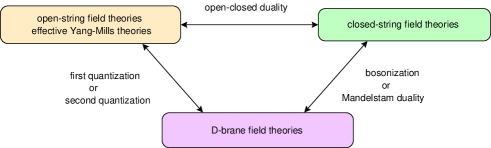
Figure 1: A trinity of dualities: D-brane field theories point toward the third possible formulation of string theory treating D-branes as elementary excitations.

As a first step to our goal, we attempt to second-quantize the Yang-Mills quantum mechanics, corresponding to the arrow on the left-hand side of this diagram. Namely, we reformulate the whole content of the Yang-Mills quantum mechanics in the Fock space which unites all different sizes of the U($N$) gauge group. As we discuss in the next section, such an attempt requires us to enlarge considerably the usual framework of field theory, especially with respect to quantum statistics.

There is another motivation for our attermpt. According to the well-known BFSS conjecture,[2] the U($N$) D0 (super) matrix quantum mechanics may also be interpreted as an exact formulation of M-theory in a special infinite-momentum frame, in which the whole system is boosted along the compactified direction, the tenth spatial dimension being a circle of radius $R_{10}=\ell_{s}g_{s}$ $\,(g_{s}\sim g_{{\rm YM}}^{2})$, with an infinitely large momentum $P_{10}=N/R\rightarrow\infty$. It is then desirable to treat $N$ as a genuine dynamical variable rather than as a mere parameter of the theory. The large $N$ limit involved here is not the usual planar limit with $g_{s}N$ begin kept fixed. Also in this aspect, it seems worthwhile to pursue an entirely new approach in which the Yang-Mills quantum mechanics is formulated in a completely unified way for all different $N$. We can hope for example that if one could find the description of the same theory in general Lorentz frame in eleven dimensional space-time, the resulting theory would necessarily include anti-D0 branes in addition to D0 branes when it is reduced to ten dimensions.

2 Gauge invariance as the quantum-statistical symmetry

From the viewpoint of second-quantization, the Yang-Mills quantum mechanics exhibits a peculiar feature with respect to quantum-statistical symmetry. In usual $N$-particle quantum mechanics in the configuration-space formulation, the wave function $\Psi(x^{i}_{1},x^{i}_{2},\ldots,x^{i}_{N})$ involves $N$ (vector) coordinates $x^{i}_{a}\,(a=1,2,\ldots,N)$ and other necessary variables of each particle. Depending on bosons or fermions, the wave functions must be totally symmetric or anti-symmetric with respect to arbitrary permutation of particles. In the Yang-Mills quantum mechanics for D particles, the coordinates of particles are replaced by $N\times N$ (vector) matrices $X^{i}_{ab}$, and the wave function $\Psi[X^{i}_{ab}]$ must be invariant under continuous U($N$) transformations,

$$X^{i}_{ab}\rightarrow\left(X^{i}\right)^{U(N)}_{ab}=\left(U(N)X^{i}U^{-1}(N)\right)_{ab}.$$ (1)

When we set the off-diagonal elements of the matrices to zero, the U($N$) transformations are restricted to the discrete permutation group S_N as a subgroup of U$(N)$. Thus, the role of permutation symmetry in ordinary particle quantum mechanics is now played by the continuous gauge symmetry. This reflects an essential feature of string theory that motion and interaction are inextricably connected by its intrinsic symmetry.

In the usual second-quantization in which the above wave function appears as a coefficient in superposing base-state vectors in the Fock space as

$$|\Psi\rangle=\frac{1}{N!}\Big{(}\prod_{a=1}^{N}\int d^{d}x_{a}\Big{)}\Psi(x_{1},x_{2},\ldots,x_{N})\psi^{\dagger}(x_{N})\psi^{\dagger}(x_{N-1})\cdots\psi^{\dagger}(x_{1})|0\rangle,$$ (2)

the validity of the canonical commutation relations for the field operators crucially depend on the permutation symmetry: $[\psi(x),\psi^{\dagger}(y)]=\delta^{d}(x-y),\quad[\psi(x),\psi(y)]=0=[\psi^{\dagger}(x),\psi^{\dagger}(y)],$ resulting

$$\psi^{\dagger}(x_{N})\psi^{\dagger}(x_{N-1})\cdots\psi^{\dagger}(x_{1})|0\rangle=\psi^{\dagger}(x_{P(N)})\psi^{\dagger}(x_{P(N-1)})\cdots\psi^{\dagger}(x_{P(1)})|0\rangle$$ (3)

and

$$\psi(y)\psi^{\dagger}(x_{N})\cdots\psi^{\dagger}(x_{1})|0\rangle={1\over(N-1)!}\sum_{P}\delta^{d}(y-x_{P(N)})\psi^{\dagger}(x_{P(N-1)})\cdots\psi^{\dagger}(x_{P(1)})|0\rangle$$ (4)

where the summation is over all permutations $(12\ldots N)\rightarrow(a_{1}a_{2}\ldots a_{N}),P(k)=a_{k}$. Here for definiteness we assumed the Bose statistics.

In the case of D particles, in addition to the fact that the permutation symmetry is replaced by the continuous unitary symmetry (1), the number of the coordinate-like degrees of freedom depends nonlinearly on $N$: the increase of the matrix-degrees of freedom from an $N$-particle system to an $(N+1)$-particle system is $d(2N+1)=d((N+1)^{2}-N^{2})$. Evidently, these features cannot be formulated in the standard canonical framework. We take this difficulty as a clue for exploring a new possible language for describing string/M theory, especially the aspect of the open-closed string duality, non-perturbatively without relying upon the world-sheet picture.

We now describe our proposal. In analogy to the usual second quantization, we first introduce ‘agents’, denoted by $\phi^{\pm}[z,\bar{z}]$, which play the role of quantum fields creating ($+$) or annihilating ($-$) one D0 brane. Here, $(z^{i},\bar{z}^{i})=\{z_{1}^{i},\bar{z}_{1}^{i},z_{2}^{i},\bar{z}_{2}^{i},\ldots\}$ is an infinite-component (complex) spatial vector as the base space of our non-relativistic field theory at a fixed time. The matrix coordinates are embedded in this infinite-dimensional space as follows: the components of the $N\times N$ matrices are identified with the components of the complex coordinates, suppressing the vector indices, as

$$z^{(b)}_{a}\equiv x_{a}^{(b)}+iy_{a}^{(b)}=X_{ab}=\bar{X}_{ba}\quad\mbox{for}\quad b\geq a,$$ (5)

which is to be interpreted as the $a$-th component of the coordinates of the $b$-th D particle. An implicit assumption here is that the field algebra, if any, should be set up such that we can effectively ignore the components $z^{(b)}_{a}$ and $\bar{z}^{(b)}_{a}$ with $a>b$ for the $b$-th operation of adding the D0 branes as dummy variables in describing the systems with a finite number of D particles. Thus in the 4-body case, for example, a $4\times 4$ matrix coordinates are reorganized into an array of four complex vectors,

$$z^{(1)}=\begin{pmatrix}x_{1}^{(1)}\cr\cdot\cr\cdot\cr\cdot\cr\cdot\cr\cdot\cr\end{pmatrix},\quad z^{(2)}=\begin{pmatrix}z_{1}^{(2)}\cr x_{2}^{(2)}\cr\cdot\cr\cdot\cr\cdot\cr\cdot\cr\end{pmatrix},\quad z^{(3)}=\begin{pmatrix}z_{1}^{(3)}\cr z_{2}^{(3)}\cr x_{3}^{(3)}\cr\cdot\cr\cdot\cr\cdot\cr\end{pmatrix},\quad z^{(4)}=\begin{pmatrix}z_{1}^{(4)}\cr z_{2}^{(4)}\cr z_{3}^{(4)}\cr x_{4}^{(4)}\cr\cdot\cr\cdot\cr\end{pmatrix}$$

The dots indicate infinitely many dummy components.

The D-particle ‘fields’ creating and annihilating a D particle connect the Fock-space states as

$$\phi^{+}:\,|0\rangle\rightarrow\phi^{+}[z^{(1)},\overline{z}^{(1)}]|0\rangle\,\rightarrow\phi^{+}[z^{(2)},\overline{z}^{(2)}]\phi^{+}[z^{(1)},\overline{z}^{(1)}]|0\rangle\,\rightarrow\cdots,$$

$$\hskip 21.33955pt\phi^{-}:\,0\,\leftarrow|0\rangle\,\leftarrow\phi^{+}[z^{(1)},\overline{z}^{(1)}]|0\rangle\leftarrow\phi^{+}[z^{(2)},\overline{z}^{(2)}]\phi^{+}[z^{(1)},\overline{z}^{(1)}]|0\rangle\leftarrow\cdots.$$

The manner in which the degrees of freedom are added (or subtracted) is illustrated in Fig. 2. Our task is then to formulate these diagrammatic operations in terms of appropriate mathematical symbols.

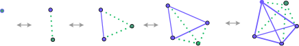
Figure 2: The D-particle coordinates and the open strings mediating them are denoted by blobs and lines connecting them, respectively. The real lines are open-string degrees of freedom which have been created before the latest operation of the creation operator, while the dotted lines indicate those created by the last operation.

3 Projection conditions and physical operators

First we have to introduce some new structures for taking into account the reduction of the components of the base-space coordinates, depending on the number of D particles. We define the following operations of projection in the infinite-dimensional base space

$$P_{n}:\,\,(w_{1},w_{2},\ldots,w_{n-1},w_{n},w_{n+1},\ldots)\rightarrow(w_{1},w_{2},\ldots,w_{n-1},r_{n},0,0,0,\ldots),$$ (6)

satisfying $P_{n}P_{m}=P_{m}P_{n}=P_{m}$ for $n\geq m.$ ($w_{n}=r_{n}+is_{n}$). If the operations are performed in the momentum space, we denote them by $\tilde{P}_{n}$ putting a tilde. Thus for arbitrary functions on the base space,

$$w_{k}f[P_{n}w,\overline{P_{n}w}]=0\quad\mbox{for}\quad k>n,\quad s_{n}f[P_{n}w,\overline{P_{n}w}]=0\,$$ (7)

or

$$\partial_{w_{k}}f[\tilde{P}_{n}w,\overline{\tilde{P}_{n}w}]=0\quad\mbox{for}\quad k>n,\quad\partial_{s_{n}}f[\tilde{P}_{n}w,\overline{\tilde{P}_{n}w}]=0.$$ (8)

The corresponding projection in the Fock space is denoted by caligraphic symbols as

$$\phi^{+}[z,\bar{z}]{\cal P}_{n}={\cal P}_{n+1}\phi^{+}[\tilde{P}_{n}z,\tilde{P}_{n}\bar{z}],\quad{\cal P}_{n}\phi^{-}[P_{n}z,P_{n}\bar{z}]=\phi^{-}[z,\bar{z}]{\cal P}_{n+1}.$$ (9)

The vacuum state vector is assumed to satisfy

$${\cal P}_{1}|0\rangle=|0\rangle,\,{\cal P}_{2}|0\rangle={\cal P}_{3}|0\rangle=\cdots=0,\quad\langle 0|{\cal P}_{1}=\langle 0|,\,\langle 0|{\cal P}_{2}=\langle 0|{\cal P}_{3}=\cdots=0.$$ (10)

At first sight, these projection conditions may look quite artificial, but should be regarded as the quantum analog of the projector property which has been known in the case of the lump solutions in the vacuum string field theory.[3] A similar feature had previously been observed in the case of non-commutative solitons.[4] In these cases, the projector property is exhibited by the classical solutions. On quantization, such classical structures must be reflected into the property of the collective coordinates, constituting the base space for soliton-fields.

It is convenient and economical to represent the multi-D-particle states by indicating only the components of the coordinates on which the field operators have nontrivial dependencies, suppressing the dummy components. We denote the effective $N$-th coordinates $(X_{1,N},X_{N,1},X_{2,N},X_{N,2},\ldots,X_{N-1,N},X_{N,N-1},X_{N,N})$ by the symbol $X_{N}$. Using this notation, the general base state of $N$-body system is expressed as

$$|N[X]\rangle\equiv{\cal P}_{N+1}[[\phi^{+}[X_{N}]\phi^{+}[X_{N-1}]\cdots\phi^{+}[X_{1}]]]|0\rangle,$$ (11)

employing a special delimiter symbol $[[***]]$ for an ordered product ($***$) of field operators, which represents the whole set of the interconnected blobs and lines for each multi-D0 state in Fig. 2.

The gauges-statistics symmetry is now expressed as the requirement

$$|N[X]\rangle\simeq|N[X^{U(N)}]\rangle.$$ (12)

Here the symbol $\simeq$ is used for the purpose of denoting that the equality is assumed to be valid when operations acting on these states are restricted to be ‘physical’. Physical operations are essentially the equivalent of gauge invariant operators in the usual first quantized formulation.

The process of adding one D0 brane is denoted by using a special symbol as

$$|(N+1)[X]\rangle=\phi^{+}[z](|N[X]\rangle)\equiv\phi^{+}[z]\triangleright|N[X]\rangle$$

$$={\cal P}_{N+2}\phi^{+}[X_{N+1}]\triangleright[[\hskip 2.5pt\phi^{+}[X_{N}]\phi^{+}[X_{N-1}]\cdots\phi^{+}[X_{1}]]]|0\rangle$$

$$={\cal P}_{N+2}[[\phi^{+}[X_{N+1}]\phi^{+}[X_{N}]\phi^{+}[X_{N-1}]\cdots\phi^{+}[X_{1}]]]|0\rangle.$$ (13)

Even though this is not a gauge invariant operation, it is useful as an intermediate tool in formulating physical operations.

On the other hand, the process of annihilating one D0 brane is expressed as

$$\phi^{-}[z,\overline{z}](|N[X]\rangle)\equiv\phi^{-}[z,\overline{z}]{\cal P}_{N+1}[[\phi^{+}[X_{N}]\phi^{+}[X_{N-1}]\cdots\phi^{+}[X_{1}]]]|0\rangle$$

$$=\phi^{-}[z,\bar{z}]{\cal P}_{N+1}\phi^{+}[X_{N}]\triangleright[[\hskip 2.5pt\phi^{+}[X_{N-1}]\phi^{+}[X_{N-2}]\cdots\phi^{+}[X_{1}]]]|0\rangle$$

$$=\int[dV(N)]\,\delta(x_{N}-X^{V(N)}_{NN})\delta^{2}(z_{1}-X^{V(N)}_{1N})\delta^{2}(z_{2}-X^{V(N)}_{2N})\cdots\delta^{2}(z_{N-1}-X^{V(N)}_{N-1,N})\sigma_{N}$$

$$\times\,{\cal P}_{N}[[\phi^{+}[X^{V(N)}_{N-1}]\phi^{+}[X^{V(N)}_{N-2}]\cdots\phi^{+}[X_{1}^{V(N)}]]]|0\rangle.$$ (14)

with $\sigma_{\ell}\equiv\delta(y_{\ell})\prod_{k>\ell}\delta^{2}(z_{k})$ corresponding to the projection condition (9) defined above. The integration volume $[dV(N)]$, which is normalized as $\int[dV(N)]=N$, over the U($N$) transformation $X_{a}\rightarrow X^{V(N)}_{a}$ is a natural generalization of the sum over all possible permutations performed in the annihilation process (4) in the usual second-quantization.

It is to be emphasized that these operations simply symbolize the processes going right or left respectively, as illustrated in Fig. 2. The multiplication rule of these field operators is maximally non-associative,[1] but can be used in order to rewrite the Yang-Mills quantum mechanics in the second-quantized language. The non-associativity is the main reason of introducing new symbols employed above. Conversely, it would not have been possible to require such a strong constraint as the gauge-statistics condition (12) unless we abandon the associativity.

We can also define bra-states by interchanging the role of $\phi^{+}$ and $\phi^{-}$ and the internal products between bra and ket states, leading to the usual probability interpretation for physical states.

As in the usual second-quantization, the whole content of configuration-space Yang-Mills quantum mechanics can be recast in terms of bilinear forms of the fields,

$$\langle\phi^{+},F\phi^{-}\rangle\equiv\int[d^{2d}z]\,\phi^{+}[z,\bar{z}]\triangleright F\phi^{-}[z,\bar{z}],$$ (15)

with $F$ being functions or operators with respect to the base-space coordinates acting on the D0 fields. For the case of functions without derivatives, we find

$$\int[d^{2d}z]\,\phi^{+}[z,\bar{z}]\triangleright F\phi^{-}[z,\bar{z}]|N[X]\rangle=\int[dU(N)]\,F[X_{1,N}^{U(N)},X_{2,N}^{U(N)},\ldots,\bar{X}_{1,N}^{U(N)},\bar{X}_{2,N}^{U(N)},$$

$$\ldots,X_{N,N}^{U(N)},0,\ldots]|N[X]\rangle,$$ (16)

the simplest example of which is the number operator with $F=1$,

$$\langle\phi^{+},\phi^{-}\rangle|N[X]\rangle=N|N[X]\rangle.$$ (17)

Another example used below is the potential term ${\rm Tr}[X^{i},X^{j}]^{2}$ appearing in the usual Hamiltonian. In terms of the bilinears, it is expressed as

$$2(\langle\phi^{+},\phi^{-}\rangle+1)(\langle\phi^{+},\Big{(}(\bar{z}^{i}\cdot z^{j})^{2}-(\bar{z}^{i}\cdot z^{j})(\bar{z}^{j}\cdot z^{i})\Big{)}\phi^{-}\rangle.$$

Remarkably, the first factor here is of order $N$ and hence that the second factor can be regarded as being well-defined in the usual large $N$ limit. It is possible to express arbitrary gauge invariants using these bilinear forms, which almost satisfy the standard algebra when acting on physical states.

4 Schrödinger equation and the large $N$ limit

Using our apparatus, the Schrödinger equation turns out to take the form ${\cal H}|\Psi\rangle=0,$ with

$${\cal H}=i(4\langle\phi^{+},\phi^{-}\rangle+1)\partial_{t}+$$

$$\hskip 42.67912pt2g_{s}\ell_{s}\Big{(}(\langle\phi^{+},\phi^{-}\rangle+1)\langle\phi^{+},\partial_{\bar{z}^{i}}\cdot\partial_{z^{i}}\phi^{-}\rangle+3\langle\phi^{+},\partial_{\bar{z}^{i}}\phi^{-}\rangle\cdot\langle\phi^{+},\partial_{z^{i}}\phi^{-}\rangle\Big{)}$$

$$+\frac{1}{2g_{s}\ell_{s}^{5}}(4\langle\phi^{+},\phi^{-}\rangle+1)(\langle\phi^{+},\phi^{-}\rangle+1)\langle\phi^{+},\Big{(}(\bar{z}^{i}\cdot z^{j})^{2}-(\bar{z}^{i}\cdot z^{j})(\bar{z}^{j}\cdot z^{i})\Big{)}\phi^{-}\rangle.$$ (18)

This is somewhat complicated. But, in the large $N$ limit and in the center-of-mass frame satisfying $\langle\phi^{+},\partial_{z^{i}}\phi^{-}\rangle=0$, it is simplified to

$$i\partial_{t}|\Psi\rangle=\Big{[}-{g_{s}\ell_{s}\over 2}\langle\phi^{+},\partial_{\bar{z}^{i}}\cdot\partial_{z^{i}}\phi^{-}\rangle-\frac{\langle\phi^{+},\phi^{-}\rangle}{2g_{s}\ell_{s}^{5}}\langle\phi^{+},\Big{(}(\bar{z}^{i}\cdot z^{j})^{2}-(\bar{z}^{i}\cdot z^{j})(\bar{z}^{j}\cdot z^{i})\Big{)}\phi^{-}\rangle\Big{]}|\Psi\rangle.$$

In terms of the M-theory parameters $R=g_{s}\ell_{s}\,,\quad\ell_{P}=g_{s}^{1/3}\ell_{s},\quad P^{+}=\langle\phi^{+},\phi^{-}\rangle/R$ after making a rescaling $(z,\bar{z})\rightarrow\left(R/\ell_{P}\right)^{-1/6}(z,\bar{z})\,,\quad t\rightarrow\left(R/\ell_{P}\right)^{-4/3}x^{+}/\ell_{P}P^{+},$ we find that the Schrödinger equation reduces to

$$P^{+}\left[P^{-}+{1\over 2\ell_{P}^{5}}\langle\phi^{+},\Big{(}(\bar{z}^{i}\cdot z^{j})^{2}-(\bar{z}^{i}\cdot z^{j})(\bar{z}^{j}\cdot z^{i})\Big{)}\phi^{-}\rangle\right]|\Psi\rangle=-{1\over 2}\langle\phi^{+},\partial_{\bar{z}^{i}}\cdot\partial_{z^{i}}\phi^{-}\rangle|\Psi\rangle,$$ (19)

which is essentially bilinear with respect to the D0 fields. This expression suggests that the potential term of the Schrödinger equation in the matrix form may now be interpreted as a light-cone component of a special external gauge field

$$A^{-}={1\over 2\ell_{P}^{5}}\left[(\bar{z}^{i}\cdot z^{j})^{2}-(\bar{z}^{i}\cdot z^{j})(\bar{z}^{j}\cdot z^{i})\right],\quad A^{+}=A_{z_{n}^{i}}=A_{\bar{z}^{i}_{n}}=0.$$

This particular form, being consistent with supersymmetry, should appear from yet unknown covariant theory through a light-cone gauge fixing.

5 Conclusion

What we have discussed in this talk is a first step towards a new framework of D-brane field theory. There remain innumerable challenging questions. An immediate problem would be to study solutions to (19). Regarding more fundamental questions, we should explore among others (i) possibility of ‘transcendental’ operator algebra associated with the continuous statistics and projection conditions; (ii) principle for making the whole formalism covariant, especially in eleven dimensional interpretation towards quantum ‘M’-field theory; (iii) ‘bosonization’ method through which the eleven dimensional supergravity as effective low-energy theory or more ambitiously closed-string field theory in ten dimensions would result.

I would like to thank the organizers for inviting me to this wonderful conference. The present work is support in part by by Grants-in-Aid for Scientific Research [No. 16340067 (B)] from the Ministry of Education, Science and Culture of Japan.

References

• [1] T. Yoneya, Prog. Theor. Phys. 135-167(2007), arXiv: 0705:1960[hep-th]; for other motivations from space-time uncertainty, see also Prog. Theor. Phys. Suppl. 171(2007)87-98. arXiv:0706.0642[hep-th].
• [2] T. Banks, W. Fschler, S. Shenker and L. Susskind, Phys. Rev. D55(1997)5112[hep-th/9610043].
• [3] L. Rastelli, A. Sen and B. Zwiebach, Adv. Theor. Math. Phys. 5(2002)353 [hep-th/0012251].
• [4] See, e. g. J. A. Harvey, P. Kraus, F. Larsen and E. J. Martinec, JHEP 0007(2000)042 [hep-th/0005031] and references therein.