Experimental continuation of periodic orbits through a fold

Abstract

We present a continuation method that enables one to track or continue branches of periodic orbits directly in an experiment when a parameter is changed. A control-based setup in combination with Newton iterations ensures that the periodic orbit can be continued even when it is unstable. This is demonstrated with the continuation of initially stable rotations of a vertically forced pendulum experiment through a fold bifurcation to find the unstable part of the branch.

Characterizing a nonlinear dynamical system typically requires the systematic investigation of stable and unstable steady-states and periodic orbits in the relevant parameter region of the system. When a mathematical model is available this task can be tackled efficiently by performing a bifurcation analysis with the method of numerical continuation. It allows one to find and follow (or continue) solutions when varying a parameter — a technique that can also be used to map out stability boundaries (bifurcations) in multiple parameters. Several software packages are available for this task; see the review papers Doedel (2007); Govaerts and Kuznetsov (2007) as an entry point to the literature.

In physical experiments the use of continuation methods has proved much more difficult. One approach is a combination of system identification and feedback control as applied by Abed et al. (1994); Siettos et al. (2004) to equilibria. In principle, it is also applicable to periodic orbits Ott et al. (1990) but, as is reported in van de Water and de Weger (2000), these methods do not generally work well when applied to real physical experiments. An alternative is extended time-delayed feedback (ETDF) Pyragas (1992, 2001), where the system is subject to a feedback loop with a delay that is given by the period of the periodic orbit one wishes to stabilize. This approach avoids system identification and, thus, is easier to implement in real experiments Schikora et al. (2006); see also the recent collection of reviews Schöll and Schuster (2007).

An important prototype problem for experimental continuation is the continuation of a stable periodic orbit through a fold (saddle-node bifurcation). As one varies a system parameter the stable periodic orbit gradually loses stability and then becomes unstable as it ‘turns around’ at the fold point. One problem is that ETDF and its modifications such as described in Pyragas (2001) do not converge uniformly near a fold of periodic orbits, meaning that they can generally not be used for tracking through a fold point; for a treatment of the autonomous case see Fiedler et al. (2007).

We present and demonstrate here a continuation method that can be used directly in an experiment to continue periodic orbits irrespective of their stability. Our method does not require a mathematical model nor the setting of specific initial conditions. Instead it relies on standard feedback control. The feedback reference signal is updated by a Newton iteration that converges to a state where the control becomes zero. The general ideas behind this method are described and tested extensively in simulations in Sieber and Krauskopf (2008a).

The implementation of feedback control requires one to measure some output of the experiment with sufficient accuracy and to provide input into the experiment in a tunable way. This requirement is quite naturally satisfied, for example, for experiments in chemistry Siettos et al. (2004); Petrov et al. (1994) and on electrical circuitry Just et al. (1997), as well as for hybrid stability tests in engineering. This type of test, where a mechanical laboratory experiment of a critical component is coupled bidirectionally to a numerical model of the remainder of the tested system Blakeborough et al. (2001), is the motivating application behind the development of experimental continuation methods Sieber and Krauskopf (2008b).

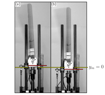
Figure 1: Photographs taken during continuation tests showing when the pendulum is at the top of a stable (a) and an unstable (b) rotation; the horizontal line ($y_{m}=0$) denotes the zero position.

The goal of this paper is to demonstrate that our method can indeed be used in an actual experiment to track periodic orbits reliably through folds to reveal branches of unstable orbits. To this end, we consider a classical mechanical experiment: the vertically forced pendulum.

In our experiment, a pendulum is attached to a pivot that moves vertically along a trajectory $y_{m}(t)$, which is controlled via a servo-mechanical actuator; this setup is as presented in Gonzalez-Buelga et al. (2007) and shown in the photos in figure 1. The actuator takes a reference trajectory $y_{r}(t)$ as its input signal and aims to match its output displacement $y_{m}(t)$ to this reference signal $y_{r}(t)$. If

$$y_{r}(t)=p\sin(\omega t)$$ (1)

then the pendulum is harmonically forced in the vertical direction with forcing frequency $\omega$ and forcing amplitude $p$. The internal dynamics of the actuator translating the reference $y_{r}$ into the actual motion $y_{m}$ is only known approximately. However, when $\omega$ is less than $10\,\mathrm{Hz}$ and if the forces exerted by the pendulum are small, the output $y_{m}$ closely follows $y_{r}$ with a small time lag ($\approx 20\,\mathrm{ms}$) and a small amplitude discrepancy (less than $0.5\,\mathrm{mm}$). The dynamics of the angular displacement $\phi$ of the pendulum are approximately a single-degree-of freedom system.

We consider here the period-one rotations of the vertically forced pendulum, which are periodic orbits where the pendulum goes over the top once per forcing period. For any fixed forcing frequency $\omega$ and sufficiently large value of the forcing amplitude $p$ one finds a dynamically stable period-one rotation. A characteristic feature of the stable rotations is the in-phase relationship between the pendulum and the forcing: the pivot is up when the pendulum is in the upside-down position; see Fig. 1(a). For the same values of $\omega$ and $p$ one also finds an unstable rotation, which is in anti-phase with the forcing; see Fig. 1(b). Both rotations are born (for a given, fixed $\omega$) in a fold bifurcation at some specific value $p_{f}(\omega)$ of the forcing amplitude, where a Floquet multiplier passes through $1$. Note that the fold point $p_{f}(\omega)$ also depends on the damping; if the damping is small and viscous then $p_{f}(\omega)\sim\omega^{-1}$ for large frequencies. (In our experiment with a pendulum of approximate effective length $0.28\,\mathrm{m}$ any frequency $\omega/(2\pi)\geq 2\,$Hz is large in this sense.)

In the experiment we measure $\phi$ and record the output

$$\theta(t)=\phi(t)-\omega t\mbox{,}$$ (2)

which is periodic for a periodic rotation (period one corresponds to a period of $T=2\pi/\omega$). The rotations are feedback stabilizable by adding control to the actuator input $y_{r}$ in (1) based on the difference between the measured relative angle $\theta(t)$ and a periodic reference signal $\tilde{\theta}(t)$. Note that feedback control via $y_{r}$ cannot achieve global stabilization because the amount of control is limited by the physical restriction of the reference signal $y_{r}$ to amplitudes less than $3\,\mathrm{cm}$. However, local feedback stabilization is sufficient for our purposes. Namely, we superimpose the feedback on the harmonic forcing (1) by setting the requested pivot trajectory $y_{r}$ to the solution of

$$\ddot{y}_{r}(t)=-\omega^{2}p\sin(\omega t)+S(\phi(t))\operatorname{PD}[\theta-\tilde{\theta}](t)$$ (3)

where $S(\phi)=1/\sin\phi$ if $|\sin\phi|>0.2$ and $0$ otherwise. The factor $S$ ensures that control is only applied at non-zero rotation angles ($\phi\neq 0,\pi$). The second term in (3) is a standard proportional-plus-derivative (PD) controller defined by $\operatorname{PD}[x]=k_{p}x+k_{d}\dot{x}$ ($k_{p}=k_{d}=0.4$ in this experiment). Since the angular velocity $\dot{\phi}$ is not directly measured, the term $\dot{x}$ is approximated by a linear filter $x_{v}=N\cdot(x-x_{f})$ where $x_{f}$ is the solution of $\dot{x}_{f}=N\cdot(x-x_{f})$ and $N$ is a large quantity ($N=100$ in this experiment). Equation (3) and the filter are linear and are solved in real-time in parallel with the experiment on a dSpace DS1104 RD real-time controller board. To ensure that the solution of (3) meets the physical restrictions on the actuator amplitude ($y_{m}\leq 3\,\mathrm{cm}$) we reset $\dot{y}_{r}$ whenever $\phi=0$.

The introduction of feedback control into the experiment via (3) adds a parameter to the overall system: the (periodic) reference signal $\tilde{\theta}(t)$. We introduce the scalar parameter $\tilde{\theta}_{0}$ and determine $\tilde{\theta}(t)$ using the recursion relation (also evaluated in real time)

$$\tilde{\theta}_{h}(t) =(1-R)\tilde{\theta}_{h}(t-T)+R\,[\theta(t-T)-\operatorname{avg}[\theta](t-T)]$$

$$\tilde{\theta}(t) =\tilde{\theta}_{0}+\tilde{\theta}_{h}(t)$$ (4)

where $T=2\pi/\omega$ is the period of the forcing, $R\in(0,1]$ is a relaxation factor and $\operatorname{avg}[\theta](t)=1/T\int_{t-T}^{t}\theta(\tau)\,\mathrm{d}\tau$ is the average of the output $\theta$ over the last forcing period (it is a constant scalar for $T$-periodic functions). We define the limit

$$\Theta(p,\tilde{\theta}_{0}):=\lim_{t\to\infty}\operatorname{avg}[\theta](t),$$ (5)

which exists (and the convergence of the time profile is uniform) for all pairs $(p,\tilde{\theta}_{0})$ that are in the vicinity of the (unknown) family of rotations near fold points. Choosing $R$ closer to zero enlarges the region where the limit (5) exists but slows down the convergence.

Equation (5) defines a smooth map $\Theta:\mathbb{R}^{2}\mapsto\mathbb{R}$ that maps the system parameter pair $(p,\tilde{\theta}_{0})$ to the asymptotic average of the output of the experiment. The map $\Theta$ is not known analytically but can be evaluated for any $(p,\tilde{\theta}_{0})$ by running the experiment with control (3) and (4) until the transients have died out. In practice the limit $\Theta(p,\tilde{\theta}_{0})$ is reached after 2–3 seconds during our experimental runs.

The reference signal $\tilde{\theta}(t)$ corresponds to a natural periodic rotation of the original (uncontrolled) vertically forced pendulum if and only if the difference $\theta-\tilde{\theta}$ is zero, making the feedback control non-invasive. This is the case when the fixed point equation

$$\Theta(p,\tilde{\theta}_{0})-\tilde{\theta}_{0}=0$$ (6)

is satisfied. For parameter pairs $(p,\tilde{\theta}_{0})$ satisfying (6) the parameter $\tilde{\theta}_{0}$ is equal to the average of the phase difference between the rotation and the forcing.

Our scheme is a modification of the classical ETDF scheme Pyragas (1992); Gauthier et al. (1994). The core of this modification is the solution of the fixed point problem (6) by means of a Newton iteration. Classical ETDF corresponds for small $R$ and a fixed $p$ to a relaxed fixed point iteration $\tilde{\theta}_{0,\mathrm{new}}=(1-R)\tilde{\theta}_{0,\mathrm{old}}+R\Theta(p,\tilde{\theta}_{0,\mathrm{old}})$ for equation (6), which is known to diverge for the unstable rotations Schöll and Schuster (2007). At the fold point $(p_{f},\tilde{\theta}_{0,f})$ the partial derivative $\partial_{2}\Theta$ equals 1, and this makes the fixed-point problem (6) singular.

To overcome this singularity we embed (6) into a pseudo-arclength continuation Doedel (2007). The pairs of $(p,\tilde{\theta}_{0})$ satisfying (6) form a curve. We introduce $y=(p,\tilde{\theta}_{0})^{T}$, and extend (6) by the pseudo-arclength condition

$$y_{t}^{T}(y-y_{\mathrm{old}})=h$$ (7)

where $h$ is the (small) stepsize along the curve, $y_{\mathrm{old}}$ is the previous point along the curve and $y_{t}$ is the unit secant through the previous two points along the curve (as a practical approximation of the tangent to the curve). Equations (6) and (7) define a system of equations of the form $F(y)=0$, which is uniformly regular near the fold. It can be solved by a relaxed quasi-Newton recursion and we choose recursion with Broyden’s rank-one update; see Sieber and Krauskopf (2008a).

To start a continuation we choose a large forcing amplitude $p$ ($2\,\mathrm{cm}$). Then the stable rotation of the uncontrolled system can be found by swinging up the pendulum manually. We measure the periodic output $\theta$ and set the initial parameter $\tilde{\theta}_{0}$ to the average of this output, thus defining the initial $y=(p,\tilde{\theta}_{0})^{T}$. In the actual implementation we scale $p$ by a factor of $20$ so that both components of the vector $y$ are of order one; the approximate initial secant to the curve is set to $y_{t}=(-1,0)^{T}$.

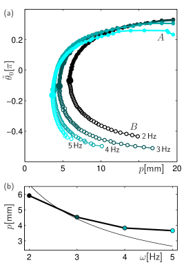
Figure 2: Experimental one-parameter bifurcation diagrams (a) for 2 Hz, 3 Hz, 4 Hz, 5 Hz, respectively, showing measured rotations (small circles: hollow for saddle rotations, full for stable rotations) and estimated fold points (large full circles). Panel (b) shows the fold points in $(\omega,p)$-plane (circles) and a viscous model estimate (thin solid line). Parameters values in (3), (4), (7) were $k_{p}=k_{d}=0.4$, $R=0.8$, $h=0.02$, and convergence tolerance $5\times 10^{-3}$.

Figure 2(a) shows four branches of rotations in the $(p,\tilde{\theta}_{0})$-plane as continued by our method. Each branch is for a different, fixed forcing frequency $\omega$ and varying forcing amplitude $p$, continued from a stable rotation near the point $A$ through the fold to an unstable rotation near the point $B$. The upper part of a branch corresponds to stable and the lower part to unstable rotations. The larger circles on each of the branches in panel (a) are the approximate values of the fold points $p_{f}(\omega)$. Figure 2(b) shows the location of the fold points in the $(\omega,p)$-plane in comparison with the theoretical prediction (thin solid curve) based on a viscous damping approximation.

Each of the four branches in Fig. 2(a) is made up of points at which the quasi-Newton recursion has converged; in practice we accept a point when the difference $\operatorname{avg}[\theta]-\tilde{\theta}_{0}$ (which is the residual of equation (6)) stays below $5\times 10^{-3}$ during one forcing period. A continuation run is performed as one continuous experiment without stopping or manual intervention; it takes about 20 minutes for a curve resolution as in Fig. 2(a). The experimental continuation stops at the lower end point of the branches, where the recursion (4) becomes unstable at a period doubling. This is a similar effect as for the classical ETDF recursion, which has been found to lose stability in a torus bifurcation Just et al. (1997).

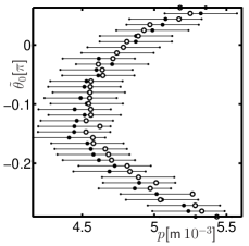
Figure 3: Variation of the phase compared to experimental accuracy near the fold for $\omega=3\,$ Hz. The error bars indicate the maximum of $|p-p_{m}|$, where $p_{m}$ is the amplitude of the pivot displacement $y_{m}$. Hollow circles: parameter $p$ as obtained by quasi-Newton iteration; full circles: $p_{m}$ as measured.

Figure 3 shows an enlargement of the branch near the fold for a forcing frequency of $\omega=3\,$ Hz. Horizontal error bars have been attached to each point (the vertical error in $\tilde{\theta}_{0}$ is invisibly small). Their size highlights the extreme difference in the scale of the axes: the range of $p$ is $1$ mm, which is of the order of a few multiples of the experimental accuracy, whereas $\tilde{\theta}_{0}$ spans a range of approximately $60$ degrees. This implies that in a small parameter region of $p$ near the fold, between $4.5\,\mathrm{mm}$ and $5.5\,\mathrm{mm}$, the average phase $\operatorname{avg}[\theta]$ of the rotation relative to the forcing changes by $60$ degrees. Thus, the fold scenario presented in Fig. 3 is an example of a very sensitive dependence of the response (the phase of the rotation) of a nonlinear dynamical system on its system parameter (the forcing amplitude $p$). This implies that the rotations shown in Fig. 3 would be extremely difficult to find by careful parameter tuning with the available experimental equipment even on the stable part of the branch near the fold. By contrast, our continuation method follows the branch of rotations through the rapid change without difficulty: the dependence of the feedback controlled pendulum on the parameter pair $(p,\tilde{\theta}_{0})$ is not sensitive and the resulting nonlinear system (6)–(7) is uniformly well-conditioned near the fold.

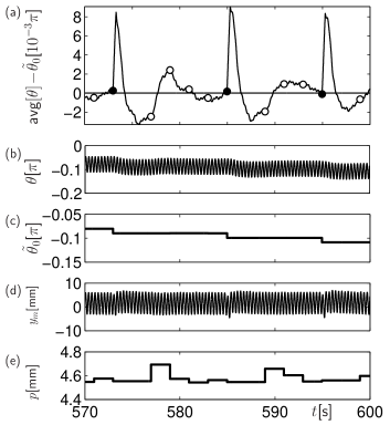
Figure 4: Time profiles during continuation for $\omega/(2\pi)=3$ Hz [(a, b, d) measured, (c, e) set by quasi-Newton iteration].

To provide more insight into how points on branches are accepted, Fig. 4 shows a $30$ s snapshot of the time profile of the experimental continuation run for $3\,$ Hz. Panel (a) shows the measured difference $\operatorname{avg}[\theta]-\tilde{\theta}_{0}$, panel (b) the output $\theta$, panel (d) the measured motion $y_{m}$ of the pivot, and panels (c) and (e) the quantities $\tilde{\theta}_{0}$ and $p$ as updated by the quasi-Newton iteration at discrete times. Filled circles in Fig. 4(a) indicate when the difference $\operatorname{avg}[\theta]-\tilde{\theta}_{0}$ is accepted as sufficiently small. Then the respective point $(p,\tilde{\theta}_{0})$ is accepted and we start the next step along the branch (by updating $y_{\mathrm{old}}$ and $y_{t}$ in the pseudo-arclength condition (7)). As a result, the difference $\operatorname{avg}[\theta]-\tilde{\theta}_{0}$ jumps briefly to a much larger value. The Newton iteration then drives the system to convergence; the open circles indicate when $\theta-\tilde{\theta}$ has been accepted as periodic. At these points $\operatorname{avg}[\theta]$ is measured and new parameters $p$ and $\tilde{\theta}_{0}$ are set to initiate the next Newton iterate.

In conclusion, we have presented a control-based continuation method and demonstrated that it is capable of tracking periodic orbits through fold bifurcations in a vertically forced pendulum experiment. Our approach does not require knowledge of an underlying mathematical model. Instead, we measure the amount of control and apply a Newton iteration to drive the control action to zero to find the next point on a branch. Importantly, this Newton iteration does not have to run in real-time, so that our method can be applied to any experiment that is feedback stabilizable. Our ongoing work focuses on control-based continuation of solutions and bifurcations in mechanical hybrid tests. It would be an interesting challenge to investigate how our approach could be extended to other application areas, such as neuroscience or cell biology, where feedback control is generally more difficult to achieve.

References

- Doedel (2007) E. Doedel, in Numerical Continuation Methods for Dynamical Systems, edited by B. Krauskopf, H. Osinga, and J. Galán-Vioque (Springer-Verlag, Dordrecht, 2007), pp. 1–49.
- Govaerts and Kuznetsov (2007) W. Govaerts and Y. Kuznetsov, in Numerical Continuation Methods for Dynamical Systems, edited by B. Krauskopf, H. Osinga, and J. Galán-Vioque (Springer-Verlag, Dordrecht, 2007), pp. 51–75.
- Abed et al. (1994) E. Abed, H. Wang, and R. Chen, Physica D 70, 154 (1994).
- Siettos et al. (2004) C. Siettos, D. Maroudas, and I. Kevrekidis, Int. J. of Bifurcation and Chaos 14, 207 (2004).
- Ott et al. (1990) E. Ott, C. Grebogi, and J. Yorke, Phys. Rev. Lett. 64, 1196 (1990).
- van de Water and de Weger (2000) W. van de Water and J. de Weger, Phys. Rev. E 62, 6398 (2000).
- Pyragas (1992) K. Pyragas, Phys. Lett. A 170, 421 (1992).
- Pyragas (2001) K. Pyragas, Phys. Rev. Lett. 86, 2265 (2001).
- Schikora et al. (2006) S. Schikora, P. Hövel, H.-J. Wünsche, E. Schöll, and F. Henneberger, Phys. Rev. Lett. 97, 213902 (2006).
- Schöll and Schuster (2007) E. Schöll and H. Schuster, eds., Handbook of Chaos Control (Wiley, New York, 2007), 2nd ed.
- Fiedler et al. (2007) B. Fiedler, V. Flunkert, M. Georgi, P. Hövel, and E. Schöll, Phys. Rev. Lett. 98, 114101 (2007).
- Sieber and Krauskopf (2008a) J. Sieber and B. Krauskopf, Nonlinear Dynamics 51, 365 (2008a).
- Petrov et al. (1994) V. Petrov, M. Crowley, and K. Showalter, Phys. Rev. Lett. 72, 2955 (1994).
- Just et al. (1997) W. Just, T. Bernard, M. Ostheimer, E. Reibold, and H. Benner, Phys. Rev. Lett. 78, 203 (1997).
- Blakeborough et al. (2001) A. Blakeborough, M. Williams, A. Darby, and D. Williams, Philosophical Transactions of the Royal Society of London A 359, 1869 (2001).
- Sieber and Krauskopf (2008b) J. Sieber and B. Krauskopf, Journal of Sound and Vibrations 315 781 (2008).
- Gonzalez-Buelga et al. (2007) A. Gonzalez-Buelga, D. Wagg, and S. Neild, Structural Control and Health Monitoring 14, 991 (2007).
- Gauthier et al. (1994) D. Gauthier, D. Sukow, H. Concannon, and J. Socolar, Phys. Rev. E 50, 2343 (1994).