1 Introduction

The Heisenberg magnet [1] is one of the very first quantum mechanical models, and it serves as the prototypical spin chain. Although it was set up almost 80 years ago it still remains a fascinating subject with many features left to be understood. Only three years after the discovery of the model and owing to its integrability, Bethe was able to write a set of equations

$$\begin{array}[b]{c}\displaystyle\left(\frac{u_{k}+{\textstyle\frac{i}{2}}}{u_{k}-{\textstyle\frac{i}{2}}}\right)^{L}=\mathop{\prod_{j=1}}_{j\neq k}^{M}\frac{u_{k}-u_{j}+i}{u_{k}-u_{j}-i}\quad\mbox{for }k=1,\ldots,M,\\[28.0pt] \displaystyle e^{iP}=\prod_{j=1}^{M}\frac{u_{j}+{\textstyle\frac{i}{2}}}{u_{j}-{\textstyle\frac{i}{2}}}\,,\qquad E=\sum_{j=1}^{M}\left(\frac{i}{u_{j}+{\textstyle\frac{i}{2}}}-\frac{i}{u_{j}-{\textstyle\frac{i}{2}}}\right),\end{array}$$ (1.1)

which determine the complete spectrum [2]. The terms “Bethe equations” or “Bethe ansatz” later became synonymous for the exact solution for generic integrable spin chain models.

Although the Bethe equations describe the complete and exact spectrum, it is virtually impossible (and perhaps not very enlightening) to solve them concretely for generic states somewhere in the middle of the spectrum. Nevertheless some corners of the spectrum are accessible (and interesting). In particular these are the low-energy and high-energy states for very long chains (the thermodynamic limit), where the Bethe equations are approximated by integral equations. Most studies have focused on the low-energy spectrum of the antiferromagnet and this regime is well-understood, see [3] for a review. For example, the antiferromagnetic state is a solution to an integral equation [4] and its excitation quanta are called spinons [5, 6].

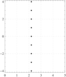
(a)

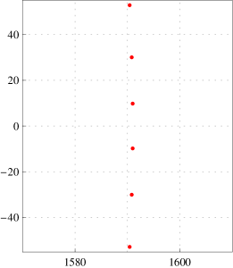
(b)

Figure 1: A Bethe string LABEL:sub@fig:bethestring and a short string LABEL:sub@fig:shortstring. Bethe strings have a strictly regular pattern and only exist on infinitely long chains. For short strings, the separation of adjacent roots is of order $\mathcal{O}(\sqrt{L})$; the string shown here lives on a chain of length $L=10,000$.

Conversely, the low-energy regime of the ferromagnet (or equivalently the high-energy regime of the antiferromagnet) is much less explored. The ferromagnetic ground state coincides with the vacuum of the Bethe ansatz, it is trivial. The excitation quanta are called magnons, and each magnon corresponds to a single Bethe root $u$ describing the rapidity of the magnon. Magnons can form bound states which are usually called Bethe strings. In a $k$-string centred at rapidity $u$ there are $k$ Bethe roots $u_{1,\ldots,k}$ arranged in a regular pattern $u_{j}=u+{\textstyle\frac{i}{2}}(k+1-2j)$, i.e. the separation of adjacent constituent magnon rapidities is $i$, see Fig. 1a. Of course this distribution pattern of Bethe roots is not exact when the length $L$ of the chain is finite and in fact large deviations are observed. Nevertheless the string hypothesis can be used to perform a counting of all states which gives the expected exact result even at finite $L$ [2] (see also [7] for a recent account including references).

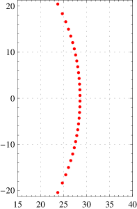
(a) $M/L=30/200$

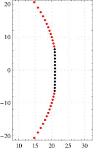
(b) $M/L=40/162$

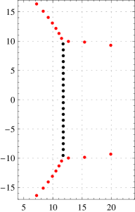
(c) $M/L=40/115$

Figure 2: Some long strings with mode number $n=1$ and various fillings $\alpha=M/L$ ($L=\text{length}$, $M=\text{number of roots}$).

An interesting type of “Bethe string” which has not found much attention until recently is one where the rapidity $u$ scales as the length $L$ of the chain. Here one distinguishes between short and long strings where the number of constituent magnons is either of $\mathcal{O}(1)$ or of $\mathcal{O}(L)$. For these strings the regular pattern is violated strongly, the distance between adjacent Bethe roots deviates much from $i$. Long strings were first investigated by Sutherland in [8]. This particular string consists of a condensate core and two tails, see Fig. 2b. Similar long strings were later considered in [9]. The distance of Bethe roots in the core is very close to $i$ while in the curved tails the density of roots decreases to $0$ at the ends. Short strings were considered in [10, 11]. Unlike for standard strings the distance of Bethe roots is of $\mathcal{O}(\sqrt{L})$, see Fig. 1b. Short strings can as well be considered as very short versions of long strings [12]. The distinction of the two types is nevertheless useful because of their different energy scales in the limit of large $L$. Furthermore, long strings can be considered as smooth classical objects for which the discrete magnon constituents play a minor role. Short strings on the other hand are quantum objects and the number of constituent magnons must be a positive integer. In fact a short string is better viewed as a coherent state of bosonic magnons. In the strict thermodynamic limit the magnons do not interact with each other, their rapidities are merely influenced by the long strings which do interact non-trivially among themselves.

Interest in the ferromagnetic regime was recently sparked by the AdS/CFT correspondence. Minahan and Zarembo showed the equivalence [11] of the spectrum of planar one-loop anomalous dimensions in the $\mathfrak{su}(2)$ sector of $\mathcal{N}=4$ supersymmetric gauge theory to the spectrum of the Heisenberg magnet with zero overall momentum. Consequently it was observed that the energies of certain long ultra-relativistic string configurations in $\mathbb{R}\times S^{3}$ [13, 14] agree precisely with the energies of certain long strings of the Heisenberg ferromagnet in the thermodynamic limit [9], see [15, 16] for reviews. This extended the earlier observation of [17] that the spectrum of magnons or short string excitations above the ferromagnetic vacuum agrees with the spectrum of quantum excitations of a short ultra-relativistic string orbiting the equator of $S^{3}$. Some time later Kruczenski related both the ultra-relativistic limit of strings on $\mathbb{R}\times S^{3}$ and the thermodynamic limit of the Heisenberg ferromagnet to one and the same Landau–Lifshitz model on $S^{2}$ [18], see also [19].

The general solution for this classical model was constructed in [20, 21] in terms of spectral curves, see [22]. It was furthermore shown that the moduli space of spectral curves of any given genus has the expected dimension. The features of the spectral curves are in one-to-one correspondence to the integral equations obtained from the above thermodynamic limit of the Bethe equations. It is therefore clear that any state of the Heisenberg ferromagnet in the thermodynamic limit is approximated by a spectral curve. Less obvious is the question if every admissible spectral curve also has a corresponding solution to the Bethe equations, and if not, what are the stability criteria? In [23] one such criterion was derived from the requirement that the mode number of a long string can be defined unambiguously and self-consistently. The statement is that the directed density $\rho$ of Bethe roots should not encircle the points $in$, $n\in\mathbb{Z}\setminus\{0\}$ when moving along the contour of a string. This is for example achieved if the density is bounded by $|\rho(x)|<1$ or $|\mathop{\mathrm{Im}}\rho(x)|<1$, i.e. the distribution of Bethe roots should not be denser than the ideal Bethe string. In particular we expect $|\rho(x)|<1$ where the cut crosses the real axis. It is in fact a natural bound for the quantum model: The values $\rho=in$ (along the imaginary axis) are distinguished because the pairwise interactions of Bethe roots in (1.1) become singular at that point. For the strictly classical model on the other hand the quantity $\rho$ does not have a meaning, and solutions with density bounded by one are not at all different from solutions where the density exceeds one. A notion of stability exists in the semiclassical theory [24]; it demands the absence of tachyonic fluctuations. This condition does not coincide with $|\rho|\leq 1$, it turns out that the latter is a stronger requirement in the case of a single cut [25].

So the question how to properly define stability remains. In this paper we would like to gain further insight into this issue by studying the general one- and two-cut solutions. The moduli space of two-cut solutions has two discrete parameters and two continuous ones, and it is sufficiently rich to investigate stability. In particular, we want to understand the role of condensate cores in the context of stability. In order to compare our analysis of the one- and two-cut spectral curves to actual solutions of the discrete Bethe equations (1.1), we further develop a numerical method for the construction of such solutions with large numbers of Bethe roots. Up to now, only few solutions that can be compared to corresponding spectral curves have been constructed [9], and they only have a comparatively small number of Bethe roots. The numerical solutions with finite numbers of Bethe roots represent quantum states on a chain of finite length and hence can also be used to examine finite-size corrections to the thermodynamic limit. For one-cut configurations these corrections were studied analytically in [23, 26, 25], some more configurations of roots were analyzed analytically and numerically in [27]. In this work we examine numerically the leading order finite-size effects explicitly for configurations beyond the one-cut case.

This paper is organised as follows. We start in Sec. 2 with a review of the general solution in the thermodynamic limit by means of spectral curves. In order to illustrate our procedure on a simple example we will first reconsider and discuss the general one-cut solution in Sec. 3. The corresponding construction within the Landau–Lifshitz model is given in App. A. Sec. 4 contains the derivation of the general two-cut solution and its properties. In Sec. 5 we will continue by applying the two-cut solution to study the issue of stability. To that end we have to determine the physical shape of the branch cuts in various regions of the parameter space. Finally in Sec. 7 we test our predictions against solutions of the Bethe equations with large but finite length, constructed numerically, in order to substantiate our claims. We conclude in Sec. 8.

2 Spectral Curves for the Heisenberg Ferromagnet

We start by reviewing the spectral curves which describe solutions of the Bethe equations (1.1) in the thermodynamic limit [21].

2.1 Baxter Equation

To derive the properties of the spectral curves it seems convenient to consider the Baxter equation as advertised in [28]

$$T(u)Q(u)=(u+{\textstyle\frac{i}{2}})^{L}Q(u-i)+(u-{\textstyle\frac{i}{2}})^{L}Q(u+i).$$ (2.1)

This equation is fully equivalent to the Bethe equations in the following way: Let $Q$ and $T$ be polynomials of degree $M$ and $L$, respectively. Then the set of solutions to the Bethe equation is equivalent to the set of Baxter equations. The Bethe roots $u_{k}$ are simply the roots of the Baxter Q-function $Q(u)=\prod_{k=1}^{M}(u-u_{k})$. Furthermore the transfer matrix eigenvalue $T(u)$ encodes the momentum eigenvalue $P$ and the energy eigenvalue $E$ in two equivalent ways as follows

$$\frac{T(u+{\textstyle\frac{i}{2}})}{(u+i)^{L}}\mathrel{} = \mathrel{}\exp\bigl{(}+iP+iuE+\mathcal{O}(u^{2})\bigr{)}+\mathcal{O}(u^{L}),$$

$$\frac{T(u-{\textstyle\frac{i}{2}})}{(u-i)^{L}}\mathrel{} = \mathrel{}\exp\bigl{(}-iP-iuE+\mathcal{O}(u^{2})\bigr{)}+\mathcal{O}(u^{L}).$$ (2.2)

In terms of the Q-function the momentum and energy read (unless $L<2$)

$$e^{iP}=\frac{Q(-{\textstyle\frac{i}{2}})}{Q(+{\textstyle\frac{i}{2}})}\,,\qquad E=\frac{iQ^{\prime}(+{\textstyle\frac{i}{2}})}{Q(+{\textstyle\frac{i}{2}})}-\frac{iQ^{\prime}(-{\textstyle\frac{i}{2}})}{Q(-{\textstyle\frac{i}{2}})}\,.$$ (2.3)

Note that for gauge theory and AdS/CFT the states are required to be cyclic, i.e. the net momentum must be zero, $e^{iP}=1$. Here we will however not restrict to cyclic states but consider states with arbitrary momentum.

Finally, the number of magnons $M$ can be read off from the transfer matrix eigenvalue expanded around $u=\infty$

$$\frac{T(u)}{u^{L}}=2+\bigl{(}{\textstyle\frac{3}{4}}L-{\textstyle\frac{1}{4}}(L-2M)(L-2M+2)\bigr{)}\frac{1}{u^{2}}+\mathcal{O}(1/u^{3}).$$ (2.4)

Note that ${\textstyle\frac{1}{4}}(L-2M)(L-2M+2)$ is the eigenvalue of the quadratic Casimir for a representation with spin ${\textstyle\frac{1}{2}}L-M$.

2.2 Thermodynamic Limit

Before we take the thermodynamic limit, we make the following substitutions: Define

$$\exp\bigl{(}ip(x)\bigr{)}=\exp(i/2x)\frac{Q(xL-{\textstyle\frac{i}{2}})}{Q(xL+{\textstyle\frac{i}{2}})}\qquad\mbox{and}\qquad t(x)=\frac{T(xL)}{(xL)^{L}}\,,$$ (2.5)

where $p(x)$ is called the quasi-momentum and $t(x)$ is the properly rescaled transfer matrix eigenvalue. It is clear that the function $p(x)$ has logarithmic singularities with opposite prefactors at $x=(u_{k}\pm{\textstyle\frac{i}{2}})/L$ and a pole with residue $i/2$ at $x=0$. Furthermore, we fix the ambiguity of $p(x)$ by shifts of $2\pi$ by setting $p(\infty)=0$. Finally, $t(x)$ is a polynomial in $1/x$ of degree $L$, i.e. it has an $L$-fold pole at $x=0$ and is analytic everywhere else. In these variables the Baxter equation reads

$$t(x)\mathrel{} = \mathrel{}(1+i/2Lx)^{L}\exp\left(-\frac{i/2}{x-i/2L}\right)\exp\bigl{(}+ip(x-i/2L)\bigr{)}$$ (2.6)

$$\mathord{}+(1-i/2Lx)^{L}\exp\left(+\frac{i/2}{x+i/2L}\right)\exp\bigl{(}-ip(x+i/2L)\bigr{)}.$$

It is now easy to take the thermodynamic limit $L\to\infty$. In this limit the magnon number is assumed to scale like $M=L\alpha$ with fixed total filling $\alpha$. The magnon rapidities scale like $u_{k}\sim L$ and are assumed to distribute smoothly along certain contours in the complex plane with distance $\mathcal{O}(L^{0})$. The distance between adjacent magnon rapidities defines the density $\rho(x)$ of Bethe roots

$$\rho(x)\approx\frac{1}{u_{k+1}-u_{k}}\,\qquad\mbox{for }u_{k}\approx u_{k+1}\approx xL.$$ (2.7)

Note that the contours typically arrange vertically in the complex plane (but not necessarily strictly along the imaginary direction). Therefore the density function $\rho(x)$ is in general complex and its phase is inversely related to the direction of the contour at the point $x$. For definiteness, let us decide that cuts generally go upwards in the complex plane, $\mathop{\mathrm{Im}}u_{k+1}>\mathop{\mathrm{Im}}u_{k}$. That means that the density will typically have a negative imaginary part, $\mathop{\mathrm{Im}}\rho(x)<0$.

The Baxter equation in the thermodynamic limit becomes simply

$$t(x)=2\cos\bigl{(}p(x)\bigr{)}.$$ (2.8)

The logarithmic singularities in $p(x)$ move together to form linear discontinuities. These discontinuities are interpreted as branch cuts connecting various Riemann sheets of $p(x)$. Apart from these and the pole at $x=0$ with residue $i/2$ the quasi-momentum $p(x)$ is analytic everywhere. The function $t(x)$ is also analytic except for an exponential singularity at $x=0$ originating from the pole of degree $L\to\infty$. Solutions $p(x),t(x)$ to the equation (2.8) with the above properties describe the spectrum in the thermodynamic limit. Let us now study the properties of the solutions in more detail.

2.3 Branch Cuts

The function $p(x)$ has discontinuities along certain branch cuts whose union shall be denoted by $\mathcal{C}$.

Density.

The discontinuity of a cut is proportional to the density $\rho(x)$ of Bethe roots (2.7) in the vicinity of the point $x$

$$\rho(x)=\frac{1}{2\pi i}\bigl{(}p(x-\varepsilon)-p(x+\varepsilon)\bigr{)},\qquad x\in\mathcal{C}.$$ (2.9)

We shall take $\varepsilon$ to be an infinitesimally small positive number, i.e. $p(x+\varepsilon)$ denotes the limiting value of $p$ at $x\in\mathcal{C}$ towards the right of the cut. Note that the combination $\mathrm{d}x\,\rho(x)$ must be real and positive which determines the direction of physical branch cuts. The integrated density along a connected cut $\mathcal{C}_{k}$ will be denoted by the filling $\alpha_{k}$

$$\alpha_{k}=\int_{\mathcal{C}_{k}}\mathrm{d}x\,\rho(x).$$ (2.10)

Standard Cut.

The function $t(x)$ must remain analytic across a branch cut of $p(x)$. Equation (2.8) tells us that $p(x)$ can change sign and shift by a multiple of $2\pi$ without causing a discontinuity in $t(x)$.

If the sign changes across a branch cut we thus have

$$p(x+\epsilon)+p(x-\epsilon)=2\pi n_{k}\qquad\mbox{for }x\in\mathcal{C}_{k},$$ (2.11)

where $n_{k}$ is the (constant) mode number associated to the connected branch cut $\mathcal{C}_{k}$. Using (2.9) we can relate the density to the quasi-momentum

$$\rho(x)=\frac{1}{\pi i}\bigl{(}p(x-\varepsilon)-\pi n_{k}\bigr{)}=\frac{1}{\pi i}\bigl{(}\pi n_{k}-p(x+\varepsilon)\bigr{)}.$$ (2.12)

This type of cut can end in a square-root singularity $x_{\ast}$ of $p(x)$ where it takes the value $p(x_{\ast})=\pi n_{k}$

$$p(x_{\ast}+\epsilon)=\pi n_{k}+\mathcal{O}(\sqrt{\epsilon})\qquad\mbox{for }x_{\ast}\in\delta\mathcal{C}_{k}.$$ (2.13)

Note that this singularity of $p(x)$ is indeed compatible with analyticity of $t(x)$ at the singularity, cf. (2.8). At $x_{\ast}$ the branch cut can be oriented in three different directions: Consider the radial coordinates $x=x_{\ast}+re^{i\varphi}$. The combination $\mathrm{d}x\rho(x)\sim e^{3i\varphi/2}\sqrt{r}\mathrm{d}r$ must be real and therefore the three possible orientations are separated by $240^{\circ}$ (where the full rotation is by $720^{\circ}$ due to the square root singularity).

Condensate Cut.

Conversely, if the sign does not change across a branch cut, the quasi-momentum must obey

$$p(x-\epsilon)-p(x+\epsilon)=2\pi n^{\prime}_{k}\qquad\mbox{for }x\in\mathcal{C}^{\prime}_{k}.$$ (2.14)

This type of cut would be required to end on a logarithmic singularity which is not compatible with analyticity of $t(x)$ in (2.8). Nevertheless such a can exist if it ends on other cuts: Indeed, we can view a logarithmic cut (2.14) as the union of two parallel standard cuts (2.11). Therefore a logarithmic cut $\mathcal{C}^{\prime}$ can split up into two parallel cuts $\mathcal{C}_{\mathrm{L}}$ (left) and $\mathcal{C}_{\mathrm{R}}$ (right) at some point, see Fig. 3. Evidence for this splitting is provided by some numerical solutions to the Bethe equations for small $L$ [10, 9]. Compatibility of (2.14) with (2.11) requires $n^{\prime}=n_{\mathrm{L}}-n_{\mathrm{R}}$. The integer $n^{\prime}_{k}$ determines the density of Bethe roots (2.9) to $\rho(x)=-in^{\prime}_{k}$ and thus a logarithmic cut has constant integral density and extends strictly along the imaginary direction.

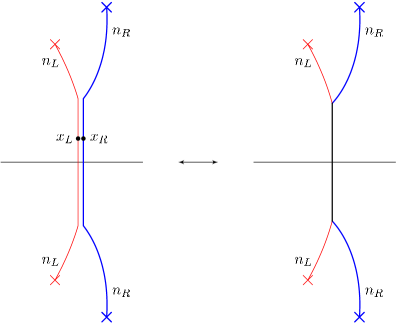
Figure 3: Two standard cuts $\mathcal{C}_{L}$ and $\mathcal{C}_{R}$ with mode numbers $n_{L}$ and $n_{R}$ whose physical contours (as determined by the condition that $\rho(x)\,\mathrm{d}x$ be real) meet at a common point. The standard cut contours start and end at square-root singularities, which are indicated by crosses. Beyond their common point, the cut contours can be placed on top of each other – the result is a condensate cut as shown in the right picture. The density $\rho_{\mathrm{c}}$ on the condensate cut can be determined by placing the individual contours infinitesimally close and parallel to each other, as shown in the left picture. It turns out that the density on the condensate cut is constant and purely imaginary: $\rho_{\mathrm{c}}(x)=i(n_{R}-n_{L})$, see (2.14). Consequently, the contour of the condensate cut must be vertical.

2.4 Observables

According to (2.3) the momentum $P$ and energy $\tilde{E}=EL$ appear in the expansion of the quasi-momentum at $x=0$

$$p(x)=\frac{1}{2x}+P+\tilde{E}x+\mathcal{O}(x^{2}).$$ (2.15)

The relation between $t(x)$ and the momentum and energy is slightly trickier: The limit of the expansion (2.1) gives two asymptotic expansions at the exponential singularity of $t(x)$ at

$$t(x)\exp(-i/2x)\mathrel{} = \mathrel{}\exp\bigl{(}+iP+ix\tilde{E}+\mathcal{O}(x^{2})\bigr{)}+\mathcal{O}(\exp(-i/x)),$$

$$t(x)\exp(+i/2x)\mathrel{} = \mathrel{}\exp\bigl{(}-iP-ix\tilde{E}+\mathcal{O}(x^{2})\bigr{)}+\mathcal{O}(\exp(+i/x)),$$ (2.16)

where the terms $\mathcal{O}(u^{L})$ in (2.1) are interpreted as exponential singularities. Putting the two expansions together and comparing with (2.8) is in agreement with (2.15).

The total filling $\alpha=M/L$ is easily obtained from the definition (2.5) of the quasi-momentum

$$p(x)=\frac{1-2\alpha}{2x}+\mathcal{O}(1/x^{2})\,.$$ (2.17)

The expansion of $t(x)$ around $x=\infty$ in (2.4) yields a compatible expression, which however does not fix the above sign

$$t(x)=2-\frac{(1-2\alpha)^{2}}{4x^{2}}+\mathcal{O}(1/x^{3}).$$ (2.18)

One can also derive two useful relations between the total and partial fillings

$$\alpha=\sum_{k}\alpha_{k}\,,$$ (2.19)

and the overall momentum and the mode numbers

$$P=\sum_{k}2\pi n_{k}\alpha_{k}\,.$$ (2.20)

2.5 Spectral Curve

For the differential $\mathrm{d}p(x)$ the analytic structure is somewhat simpler: The shifts of $p(x)$ by constants which arise when passing through a branch cut are not seen in $dp(x)$. The differential $\mathrm{d}p(x)$ thus has merely two Riemann sheets with opposite signs and it is called the spectral curve. In particular, the condensate cuts drop out in the spectral curve. Only the standard branch cuts are seen in $dp(x)$; they change the sheet or equivalently flip the sign.

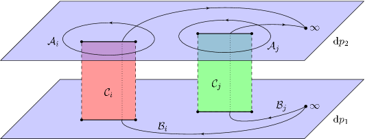
Figure 4: Cycles of the spectral curve $\mathrm{d}p$. Shown are the two sheets $\mathrm{d}p_{1}$, $\mathrm{d}p_{2}$ of the Riemann surface of the spectral curve $\mathrm{d}p$. The two sheets are connected by cuts $\mathcal{C}_{i}$. To each cut $\mathcal{C}_{i}$ is associated an A-cycle $\mathcal{A}_{i}$ and a B-cycle $\mathcal{B}_{i}$. The A-cycle encircles the cut contour, staying on the same sheet, while the B-cycle starts at $x=\infty$ on one sheet, passes through the cut and ends at $x=\infty$ on the other sheet.

The above parameters of the solution can be read off from the spectral curve. First we need to introduce A-cycles and B-cycles for the cuts. A-cycles wind around the cuts while B-cycles extend from $x=\infty$ through a cut and back to $x=\infty$ but on the other Riemann sheet, see Fig. 4.For a normal cut the A-cycle does not intersect with any branch cut of the quasi-momentum. The A-period of $\mathrm{d}p(x)$ is therefore zero

$$\oint_{\mathcal{A}_{k}}\mathrm{d}p(x)=0.$$ (2.21)

The B-period yields the mode number $n_{k}$ of the cut

$$\int_{\mathcal{B}_{k}}\mathrm{d}p(x)=2\pi n_{k}.$$ (2.22)

To understand this we split up the contour into the two parts before and after crossing the cut at point $x$. The first part yields $p(x+\varepsilon)-p(\infty)=p(x+\varepsilon)$ due to our normalisation $p(\infty)=0$. On the other sheet the sign of the quasi-momentum is flipped and consequently the second part yields $-p(\infty)+p(x-\varepsilon)=p(x-\varepsilon)$. Altogether we obtain $p(x+\varepsilon)+p(x-\varepsilon)$ and by (2.11) this equals $2\pi n_{k}$. Note that a vanishing A-period of $\mathrm{d}p$ enables us to be rather unspecific about how the B-period returns to $x=\infty$ on the second sheet.

Finally, the partial filling (2.10) of a cut can be expressed through the A-period of $x\,\mathrm{d}p(x)$

$$\alpha_{k}=\int_{\mathcal{C}_{k}}\mathrm{d}x\,\rho(x)=-\frac{1}{2\pi i}\oint_{\mathcal{A}_{k}}\mathrm{d}x\,p(x)=\frac{1}{2\pi i}\oint_{\mathcal{A}_{k}}x\,\mathrm{d}p(x).$$ (2.23)

This follows by substitution of (2.9) and partial integration. Note that the partial integration assumes that the A-period of $\mathrm{d}p$ is zero.

The above discussion shows that the cut contours and corresponding cycles can be deformed continuously without affecting the parameters of the solution. However, special care has to be taken when a cycle moves into a cut or passes through a singularity. In particular, the reality condition $\mathrm{d}\rho(x)\geq 0$ appears to play no important role in the purely classical approximation.

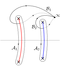
(a)

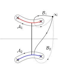
(b)

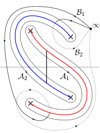
(c)

Figure 5: Possible cut contours (blue/red,thick) and corresponding cycles for a core with four tails. In the standard configuration LABEL:sub@fig:cycles.vertical, complex conjugate pairs of branch points are connected more or less directly. In this case, the A-periods vanish and the B-periods are non-ambiguous, even when the central cut segments join and form a condensate core as in Fig. 3. When the branch points are connected horizontally LABEL:sub@fig:cycles.horizontal, the mode numbers (B-periods) of the cuts are ambiguous, hence the configuration requires a condensate (black,vertical) between the two cuts. This implies that the A-periods do not vanish. Branch cuts that wind around each other LABEL:sub@fig:cycles.wild also require a condensate cut, hence complex conjugate branch points carry different mode numbers.

In the case of many cuts the assignment of cycles is not necessarily unique anymore. Let us discuss what happens when two standard cuts join to form a condensate cut with four tails. Now there are various ways in which the four branch points could be connected, see Fig. 5. The standard method to set up the cuts is to connect complex conjugate pairs of branch points more or less directly, as in Fig. 5a. Then the above assignments of parameters works well. All cuts are of the standard kind and condensate cuts arise from two standard cuts running parallel for a while, see Fig. 3.

Another option would be to connect the branch points horizontally with a condensate cut forming between the two standard cuts (Fig. 5b). This option leads to non-zero A-periods

$$\oint_{\mathcal{A}_{k}}\mathrm{d}p(x)=\pm 2\pi n^{\prime}_{j},$$ (2.24)

where $n^{\prime}_{j}$ is the density of the condensate cut being intersected by the A-cycles. The non-trivial A-cycles then lead to ambiguities in the definition of mode numbers $n_{k}$ and fillings $\alpha_{k}$. Also non-technically it is unclear how to associate suitable $n_{k}$ and $\alpha_{k}$ to these two individual cuts. The situation becomes even worse if the cuts wind around the branch points (Fig. 5c). Therefore the standard straight connection of complex conjugate pairs of branch points appears best to describe the parameters.

2.6 Finite Gap Solutions

The simplest types of spectral curves with the desired properties are the finite-gap solutions. These have finitely many branch cuts (“gaps”) and therefore finitely many branch points. The general ansatz for $p^{\prime}(x)$ is given by

$$p^{\prime}(x)^{2}=\frac{g(x)^{2}}{x^{4}h(x)}\,,$$ (2.25)

where $g(x)$ and $h(x)$ are polynomials of degree $K$ and $2K$, respectively

$$g(x)=\sum_{k=0}^{K}c_{k}x^{k},\qquad h(x)=\prod_{k=1}^{2K}(x-x_{k}).$$ (2.26)

The roots $x_{k}$ are the square root branch points which must come in (complex conjugate) pairs. A pair is typically connected by a branch cut and therefore $K$ is the number of standard branch cuts. The genus of the algebraic curve $p^{\prime}(x)$ equals $g=K-1$.

2.7 Stability

Stability addresses the question which classical spectral curves with real and positive densities on the cuts can be realised approximately by solutions of the Bethe equations with large but finite $L$. An important stability criterion was derived in [23]

$$\int_{\mathcal{C}_{k}}d\log\frac{n+i\rho(x)}{n-i\rho(x)}=0\quad\mbox{for all }n\in\mathbb{Z}.$$ (2.27)

The criterion implies that the branch of the above logarithm can be uniquely defined on an isolated standard branch cut $\mathcal{C}_{k}$. The argument of the logarithm

$$\frac{n+i\rho(x)}{n-i\rho(x)}\approx\frac{n(u_{k+1}-u_{k})+i}{n(u_{k+1}-u_{k})-i}\approx\frac{u_{k+n}-u_{k}+i}{u_{k+n}-u_{k}-i}$$ (2.28)

approximates the scattering term in the Bethe equation (1.1). In a logarithmic form of the Bethe equations the condition implies that mode numbers can be unambiguously associated to the cuts, even in the full quantum theory. Unlike the classical quantities, here the density appears independently of the differential $\mathrm{d}x$ and therefore it is crucial to use the physical contour of the cut $\mathcal{C}_{k}$.

The most interesting case is $n=1$; the conditions for $n>1$ appear to be less constraining and perhaps redundant. It is quite clear that if the absolute density is bounded by unity everywhere,

$$|\rho(x)|<1,$$ (2.29)

the stability criterion will be satisfied. However this condition is too restrictive in general. Nevertheless, for a stand-alone cut the density is typically highest at the centre $x_{0}$ where the cut crosses the real axis and where the density becomes purely imaginary. It is then necessary to obey

$$|\rho(x_{0})|<1,$$ (2.30)

in order to satisfy the stability condition. Otherwise the argument of the logarithm in (2.27) will cross the negative real axis at $x_{0}$ and wind around the origin once.

What remains obscure at this point is how to interpret the stability condition for two standard cuts joined by a condensate. Also it is not clear if (2.27) alone can ensure that a given configuration of cuts can be realised by a concrete solution of the Bethe equations. In the following we shall study the general one-cut and two-cut solutions in order to shed some light on the various classically allowed configurations of cuts and when the stability condition is satisfied.

3 One-Cut Solution

In this section we review the simplest type of spectral curve with one cut. It has two parameters, the mode number $n$ and the filling $\alpha$. Its genus is zero and thus we will only encounter algebraic and trigonometric functions. We also review the corresponding construction for the Landau–Lifshitz model in App. A.

3.1 Solution

The general one-cut solution was obtained in [21]. It has one mode number $n$, one filling $\alpha$ and it takes the form

$$p(x)=\pi n+\frac{1-2\pi nx}{2x}\sqrt{1+\frac{8\pi n\alpha x}{(1-2\pi nx)^{2}}}\,.$$ (3.1)

The derivative of the quasi-momentum defines the spectral curve

$$p^{\prime}(x)^{2}=\frac{(1-2\pi nx(1-2\alpha))^{2}}{4x^{4}\bigl{(}(1-2\pi nx)^{2}+8\pi n\alpha x\bigr{)}}$$ (3.2)

and matches with (2.25,2.26). The quasi-momentum is in agreement with the expansions at $x=0,\infty$ (2.15,2.17) and with the condition for the branch points (2.13). The higher terms in the expansion at $x=0$ yield the total momentum and energy

$$P=2\pi n\alpha,\qquad\tilde{E}=4\pi^{2}n^{2}\alpha(1-\alpha).$$ (3.3)

If we choose to restrict to cyclic states as required for AdS/CFT we have to set $P=2\pi m$ with integer $m$. Then the total filling must be a rational number $\alpha=m/n$. However, all these solutions are unstable. As we shall see later this is related to the fact that the total momentum leaves the first Brillouin zone, $|P|>\pi$.

3.2 Cut Contour

The physical contour of the cut is not a simple function. In particular, it is not given by the natural branch cut of the square root in $p(x)$; it lies somewhat closer to the origin. In order to find the contour, we shall make use of the identity (2.12) which relates the density to the quasi-momentum. The integrated density must be real and positive; therefore we will need the integral of the quasi-momentum

$$\mathnormal{\Lambda}(x)=\int p(x)\,\mathrm{d}x\mathrel{} = \mathrel{}\pi nx+\frac{1-2\pi nx}{2}\sqrt{1+\frac{8\pi n\alpha x}{(1-2\pi nx)^{2}}}$$ (3.4)

$$\mathord{}-\mathop{\mathrm{artanh}}\left(\frac{1-2\pi nx}{1+2\pi nx}\sqrt{1+\frac{8\pi n\alpha x}{(1-2\pi nx)^{2}}}\right)$$

$$\mathord{}-\alpha\mathop{\mathrm{arcoth}}\left(\frac{1-2\pi nx}{1-2\pi nx-2\alpha}\sqrt{1+\frac{8\pi n\alpha x}{(1-2\pi nx)^{2}}}\right).$$

On the cut the combination $\mathnormal{\Lambda}(x)-\pi nx$ must be real. At the branch points

$$x_{\pm}=\frac{1-2\alpha\pm 2i\sqrt{\alpha(1-\alpha)}}{2\pi n}$$ (3.5)

it takes the values $\mathnormal{\Lambda}(x_{\pm})-\pi nx_{\pm}=\pm{\textstyle\frac{i}{2}}\pi\alpha$ and thus the contour is defined by $\mathnormal{\Lambda}(x)-\pi nx\in{\textstyle\frac{i}{2}}\pi\alpha[-1,1]$. In Fig. 6 we have plotted the contour of a sample cut.

In fact as discussed below (2.13), a branch cut with positive density can, in principle, originate from a branch point in three different directions. The shortest path will turn out to be the only physical choice.

The longer circular path which encircles the origin is equivalent to the one-cut solution with opposite mode number $n^{\prime}=-n$ and conjugate filling $\alpha^{\prime}=1-\alpha$. This can be seen as follows: We deform the shorter cut continuously to the longer cut by rotating it towards the right by $240^{\circ}$. At some point the cut has to pass the point $x=\infty$. This has the following two effects. Firstly, the A-cycle describing the filling (2.23) intersects $x=\infty$ twice. This adds to $\alpha$ the residues ${\textstyle\frac{1}{2}}-\alpha$ and ${\textstyle\frac{1}{2}}-\alpha$ (the opposite sheet with opposite circulation) so we obtain $\alpha^{\prime}=\alpha+2({\textstyle\frac{1}{2}}-\alpha)=1-\alpha$. Secondly, the point $x=\infty$ now resides on a different sheet. This implies $p(\infty)=2\pi n$ and we have to subtract the constant $2\pi n$ to normalise to $p(\infty)=0$. At the branch point that leads to $p(x_{\ast})=-\pi n$, i.e. the new mode number is $n^{\prime}=-n$. Note that this configuration has a large filling $\alpha\geq{\textstyle\frac{1}{2}}$ because the shorter cut has $\alpha\leq{\textstyle\frac{1}{2}}$. It is therefore unphysical.

For the third choice we rotate the contour towards the left by $240^{\circ}$. This contour escapes towards $\pm i\infty$ on both sides. Moreover the density $\rho$ on the contour approaches a finite value at infinity. Therefore the total filling on the contour is infinite, and the configuration is inconsistent.

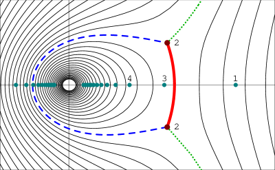
Figure 6: Physical position of the cut (solid/red) for a one-cut solution with $n=2$, $\alpha=0.05$. Two alternative contours with positive filling originating from the same branch points are shown: The second (dashed/blue) contour corresponds to the conjugate one-cut solution with $n=-2$, $\alpha=0.95$. This contour is unphysical because the filling exceeds $0.5$. The third contour (dotted/green) extends to infinity, it is inconsistent because the filling is infinite. The remaining lines depict possible cuts with real filling not ending on the branch points. Fluctuation points are marked by dots.

3.3 Stability

We are now ready to consider the issue of stability. The stability condition for the one-cut solutions implies that the density must be bounded by unity where the cut crosses the real line. Assume the cut crosses the real axis at $x_{0}$ which must be the solution of the equation $\mathnormal{\Lambda}(x_{0})=\pi nx_{0}$. This equation is transcendental and we can only solve it numerically for given values of $n$ and $\alpha$. Once we have the value $x_{0}$ the absolute density is given by

$$\bigl{|}\rho(x_{0})\bigr{|}=\frac{1}{\pi}\,\bigl{|}p(x_{0})-\pi n\bigr{|}.$$ (3.6)

The density for solutions with $n=1$ is plotted in Fig. 7.

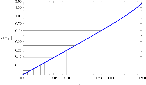
Figure 7: Absolute density $|\rho(x_{0})|$ at the centre of a single cut with mode number $|n|=1$ versus the cut’s filling fraction $\alpha$ (blue/thick). Also displayed are the lines $1/m$ for integer $m$. According to equation (3.7), the intersection points of these lines with the density mark the maximal fillings $\alpha_{\mathrm{cond}}$ of stable solutions with mode numbers $m$ (see also Tab. 1).

We are interested in the filling $\alpha_{\mathrm{cond}}$ where the density reaches the maximum allowed value, $|\rho(x_{0})|=1$ or $p(x_{0})=\pi(n+1)$. Let us assume for simplicity that $n>0$. Because of the way $p(x)$ and $\mathnormal{\Lambda}(x)$ scale with $x$ and $n$, the intersection point of a cut with mode number $n$ and filling $a$ and the density at that point are directly related to the intersection point and the density of the cut with mode number $1$ and the same filling:

$$x_{0}(n,\alpha)=\frac{x_{0}(1,\alpha)}{n}\,,\qquad\rho_{n}(x_{0}(n,\alpha))=n\rho_{1}(x_{0}(1,\alpha))\,.$$ (3.7)

Hence it is sufficient to obtain the fillings $\alpha$ at which the absolute density at the centre of the cut with mode number $1$ equals $1/n$. These fillings are exactly the maximal fillings of the cuts with mode number $n$ that are allowed by the stability criterion; they are indicated in Fig. 7.

Alternatively, one can solve the equation $p(x_{0})=\pi(n+1)$ for $x_{0}$ in terms of $\alpha$ and $n$. The solution is substituted in $\mathnormal{\Lambda}(x_{0})=\pi nx_{0}$ which yields the equation

$$2(q+n)\mathop{\mathrm{arcoth}}(q+2n)-\frac{1-q^{2}}{2n}\mathop{\mathrm{artanh}}\left(\frac{1-q^{2}-2nq}{2n}\right)=1\,.$$ (3.8)

Here $q$ is an auxiliary variable that encodes the maximal filling $\alpha_{\mathrm{cond}}$ and the intersection point $x_{0}$

$$\alpha_{\mathrm{cond}}=\frac{1-q^{2}}{4n(q+n)}\,,\qquad x_{0}=\frac{1}{2\pi(q+n)}\,.$$ (3.9)

We list the first few values of $\alpha_{\mathrm{cond}}$ in Tab. 1. Note that $\alpha_{\mathrm{cond}}<1/2n$, which implies that stable solutions have a momentum $P<\pi$. Hence, cyclic one-cut solutions cannot be stable. In fact one can solve the above equation perturbatively using that $q\sim 1/n$. The expansion of $\alpha_{\mathrm{cond}}$ reads

$$\alpha_{\mathrm{cond}}=\frac{1}{4n^{2}}-\frac{7}{144n^{4}}+\frac{367}{38880n^{6}}-\frac{540373}{293932800n^{8}}+\frac{1895953}{5290790400n^{10}}+\mathcal{O}(1/n^{12}).$$ (3.10)

$|n|$	$\alpha_{\mathrm{cond}}$	$\tilde{E}_{\mathrm{cond}}/4\pi^{2}$
1	0.2092896452	0.1654874896
2	0.0596024470	0.2241999811
3	0.0271903146	0.2380590127
4	0.0154373897	0.2431852264
5	0.0099228217	0.2456089819

$|n|$	$\alpha_{\mathrm{cond}}$	$\tilde{E}_{\mathrm{cond}}/4\pi^{2}$
6	0.0069071371	0.2469394280
7	0.0050818745	0.2477464054
8	0.0038944180	0.2482720935
9	0.0030790284	0.2486333844
10	0.0024951483	0.2488922545

Table 1: Maximal fillings $\alpha_{\mathrm{cond}}$ and the corresponding energies $\tilde{E}_{\mathrm{cond}}$ for one-cut solutions for the first few mode numbers $n$. Above these fillings, solutions require a condensate for stability.

3.4 Fluctuations

Fluctuations are very small cuts which can exist in a background the one long cut [9]. For the one-cut solution they were discussed in [9, 29, 25]. Their position $x_{\ast}$ is determined by the long cut,

$$p(x_{\ast})=\pi n_{\ast},$$ (3.11)

but they are not strong enough to back-react on the position of the long cut substantially. We shall again assume that $n>0$. The solution to the above equation reads

$$\frac{1}{x_{\ast}}=2\pi n(1-2\alpha)+2\pi(n_{\ast}-n)\sqrt{1-\frac{4n^{2}\alpha(1-\alpha)}{(n_{\ast}-n)^{2}}}\,.$$ (3.12)

The momentum and energy of a fluctuation mode quantum with $\delta\alpha=1/L$ are given by [29, 25]

$$\delta P=\frac{2\pi n_{\ast}}{L}\,,\qquad\delta\tilde{E}=\frac{4\pi^{2}}{L}\left(n(2n_{\ast}-n)(1-2\alpha)+(n_{\ast}-n)^{2}\sqrt{1-\frac{4n^{2}\alpha(1-\alpha)}{(n_{\ast}-n)^{2}}}\right).$$ (3.13)

If the long cut is rather short, the fluctuations will reside close to their vacuum positions $x_{\ast}\approx 1/2\pi n_{\ast}$. For fluctuations of the same mode number as the cut, $n_{\ast}=n$, the condition $p(x_{\ast})=\pi n_{\ast}$ is solved by the branch points, which means that this particular fluctuation will increase the size of the long cut. The longer the long cut gets the more will it attract fluctuations with nearby mode numbers $n_{\ast}\approx n$ towards it [25]. At some value of $\alpha$, the fluctuation with $n_{\ast}=n+1$ collides with the long cut (from the left). This happens precisely when the density reaches unity at the real axis, cf. (3.6), and so the above discussion applies. Note that at this point the fluctuation with $n_{\ast}=n-1$ is still at some distance from the cut.

In conclusion, we can infer that for all stable one-cut solutions the fluctuations are well-separated from the long cut. When the fluctuation collides with the cut we can actually argue independently for an instability: Now the long cut can be filled not only from both ends, but also from the middle. In practice we expect that a condensate cut (with unit density) will form in the middle of the long cut.

3.5 Condensate Formation

Let us add a vertical condensate cut ending on the existing branch cut, see Fig. 8. This is achieved by shifting the quasi-momentum $p(x)$ by $-2\pi$ in the region enclosed by the two contours, cf. Fig. 9. Clearly the new curve satisfies all conditions for the classical spectral curve. In effect, the shift decreases the mode number on the inner part of the original branch cut by one unit according to (2.11). Furthermore, the density function is changed according to (2.9,2.12) and thus the inner part of the branch cut has to be moved to obtain a real density

$$\rho(x)=\frac{1}{\pi i}\bigl{(}\pi(n-1)-p(x+\varepsilon)\bigr{)}.$$ (3.14)

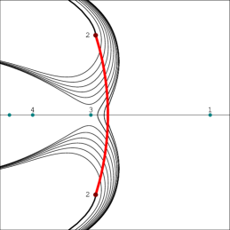
(a) $\alpha<\alpha_{\mathrm{cond}}$

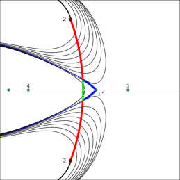
(b) $\alpha_{\mathrm{cond}}<\alpha<\alpha_{\mathrm{crit}}$

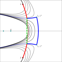
(c) $\alpha_{\mathrm{crit}}<\alpha$

Figure 8: Potential deformations (thin/black) of a branch cut (solid/red) after inserting a condensate (dashed/green) for $n=2$ and LABEL:sub@fig:onebubblecutsa $\alpha=0.03$, LABEL:sub@fig:onebubblecutsb $\alpha=0.065$, LABEL:sub@fig:onebubblecutsc $\alpha=0.8$. The physical deformation (solid/blue) exists only for $\alpha>\alpha_{\mathrm{crit}}$. The contours originating from near the ends of the branch cut close up after encircling the origin.

The condensate cut can end on any point of the branch cut, and we show the various potential configurations in Fig. 8. Any of these configurations with a condensate appear to be possible from the point of view of spectral curves. However, the Bethe equations will single out one particular configuration as the distribution of Bethe roots in the thermodynamic limit. To understand the physical distribution we have to distinguish three qualitatively different cases, see Fig. 8.

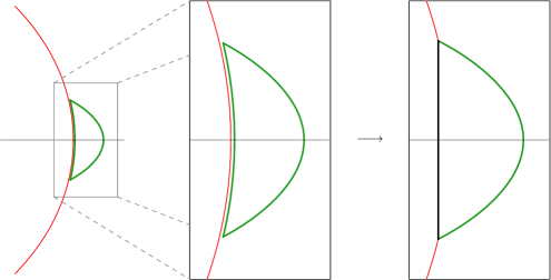
Figure 9: Possible deformation of a branch cut: For large enough filling $\alpha>\alpha_{\mathrm{cond}}$, a closed loop cut (thick/green) can be added to the branch cut (thin/red). In the region enclosed by the loop cut, the quasi-momentum $p(x)$ is changed to $-p(x)+2\pi n_{\mathrm{L}}$, where $n_{\mathrm{L}}$ is the mode number of the loop cut. As shown in Fig. 3, the density $\rho_{\mathrm{C}}$ on the common part of the two contours equals $i(n_{\mathrm{L}}-n_{\mathrm{B}})$, where $n_{\mathrm{B}}$ is the mode number of the branch cut. Hence the resulting configuration has a condensate core, as shown in the right Figure.

In the first case the filling is below the threshold for condensate formation, $\alpha<\alpha_{\mathrm{cond}}$, as discussed in the previous subsections. Here all potential deformations leave the branch cut almost vertically and then circle around the origin. Due to the residue at the origin the filling of the configuration is altered and becomes larger than ${\textstyle\frac{1}{2}}$. Inserting a condensate cut therefore leads to an unphysical configuration when $\alpha<\alpha_{\mathrm{cond}}$.

At $\alpha=\alpha_{\mathrm{cond}}$ the fluctuation point with mode number $n_{\ast}=n+1$ crosses the branch cut and effectively acquires the mode number $n_{\ast}=n-1$. We now have two fluctuation points with the same mode number $n-1$. For definiteness, let us call the new point $n_{\ast}=(n-1)^{\prime}$. When increasing $\alpha$ further, it will eventually collide with the other fluctuation point. This happens at $\alpha=\alpha_{\mathrm{crit}}$ with

$$\alpha_{\mathrm{crit}}=\frac{1}{2}-\frac{1}{2}\sqrt{1-\frac{1}{n^{2}}}\,.$$ (3.15)

Consider now the case $\alpha_{\mathrm{cond}}<\alpha<\alpha_{\mathrm{crit}}$. The deformations originating from the branch cut can now have two qualitatively different shapes. The contours originating from near the ends of the branch cut behave like in the first case above and are thus unphysical. The contours originating from near the centre however are just small deformations of the original cut and consequently they lead to the same filling. All of these configurations are in principle okay, however, only one can be physical. Indeed one of the configurations is special: the limiting shape, i.e. the largest possible small deformation. It is distinguished by a cusp at the fluctuation point for $n_{\ast}=(n-1)^{\prime}$, see Fig. 8b. We can argue that this is the physical configuration: When we add macroscopically many Bethe roots to the fluctuation point, it will split up and form two square root singularities. The deformed cut will split at the cusp and form a condensate with four tails as in Fig. 10b. This configuration is a genuine two-cut solution as we shall see in the next section. When we take the new Bethe roots away we should return to the one-cut solution. This is possible only if the deformed contour meets the fluctuation point with mode number $n_{\ast}=(n-1)^{\prime}$, as in Fig. 8b,10a. In conclusion the one-cut solution for $\alpha_{\mathrm{cond}}<\alpha<\alpha_{\mathrm{crit}}$ is a degenerate case of a two-cut solution.

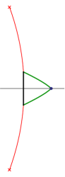
(a)

(b)

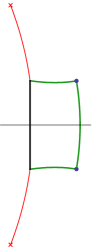
(c)

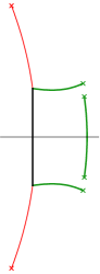
(d)

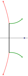
(e)

Figure 10: For large fillings $\alpha$, one-cut solutions are degenerate cases of two- and three-cut solutions. When a macroscopic number of Bethe roots gets added to the fluctuation point (blue dot) in LABEL:sub@fig:onecut2, two square-root branch points form, the closed loop cut splits at its cusp and yields a genuine two-cut solution LABEL:sub@fig:onecut2reg. This singles out the deformation shown in LABEL:sub@fig:onecut2 as the physical one for the case $\alpha_{\mathrm{cond}}<\alpha<\alpha_{\mathrm{crit}}$. At even higher fillings $\alpha>\alpha_{\mathrm{crit}}$ LABEL:sub@fig:onecut3 an excitation of the fluctuation points results in a three-cut solution LABEL:sub@fig:onecut3reg. A local minimum of the energy is reached when all roots from the third cut are moved to the second, leaving a two-cut configuration and a bare fluctuation point as in LABEL:sub@fig:onecut32.

The final case is $\alpha_{\mathrm{crit}}<\alpha$. Here the two fluctuation points with mode numbers $n_{\ast}=(n-1)^{\prime}$ and $n_{\ast}=(n-1)$ have joined and branched off into the complex plane. The configurations are similar to the above case of $\alpha_{\mathrm{cond}}<\alpha<\alpha_{\mathrm{crit}}$, but now the limiting shape meets both fluctuation points and thus has two cusps joined by an approximately vertical contour. In this case we cannot add Bethe roots to any of the two fluctuation points individually because it would violate the reality condition (reflection symmetry of the configuration about the real axis). They can only be excited in pairs to create four new square root singularities and a three-cut solution as in Fig. 10d. In other words, the configuration is a degenerate case of a three-cut solution. The third cut is the line segment joining the two fluctuation points. By removing Bethe roots from this cut one lowers the energy and we might therefore call this solution unstable. Nevertheless we expect it to be a perfectly well-behaved solution of the Bethe equations in the thermodynamic limit albeit with non-minimal energy. A local minimum is obtained by shifting all Bethe roots from the third cut to the second, as in Fig. 10e. This is a true two-cut solution which will be discussed in generality in the next section.

Finally we remark that for $n=1$ the third case does not exist because $\alpha_{\mathrm{crit}}={\textstyle\frac{1}{2}}$. This is because the fluctuation point with $n_{\ast}=0$ is always at $x_{\ast}=\infty$ and cannot join with the one for $n_{\ast}=0^{\prime}$. Therefore the solution with $n=1$ represents a local minimum of the energy for all $0<\alpha<1/2$.

4 The General Two-Cut Solution

As described in Sec. 2, a solution to the Bethe equations (1.1) in the thermodynamic limit is given by a quasi-momentum $p$, whose domain is a multi-sheeted cover of $\bar{\mathbb{C}}$. The corresponding spectral curve $\mathrm{d}p$ has B-periods in $2\pi\mathbb{Z}$ and vanishing A-periods, while the quasi-momentum $p(x)$ has a simple pole of residue $1/2$ at $x=0$. In this section, the general spectral curve with two cuts will be constructed and its properties will be investigated. Spectral curves with two cuts have a Riemann surface of genus one and thus can be described in terms of complete elliptic integrals of the first, second and third kind. These are denoted by $\mathop{\smash{\operator@font K}\vphantom{a}}\nolimits$, $\mathop{\smash{\operator@font E}\vphantom{a}}\nolimits$ and $\mathop{\smash{\operator@font\Pi}\vphantom{a}}\nolimits$ and are defined as

$$\mathop{\smash{\operator@font K}\vphantom{a}}\nolimits(q) :=\int_{0}^{1}\frac{1}{\sqrt{(1-t^{2})(1-qt^{2})}}\,\mathrm{d}t\,,$$

$$\mathop{\smash{\operator@font E}\vphantom{a}}\nolimits(q) :=\int_{0}^{1}\frac{\sqrt{1-qt^{2}}}{\sqrt{1-t^{2}}}\,\mathrm{d}t\,,$$

$$\mathop{\smash{\operator@font\Pi}\vphantom{a}}\nolimits(z\mathpunct{|}q) :=\int_{0}^{1}\frac{1}{(1-zt^{2})\sqrt{(1-t^{2})(1-qt^{2})}}\,\mathrm{d}t\,.$$ (4.1)

The two-cut solution can be obtained by direct integration of the general ansatz (2.25). Here a different approach will be followed which makes use of the result obtained for the symmetric case in [30].

4.1 The Symmetric Two-Cut Solution

We will obtain the general two-cut solution by generalising the symmetric solution [31, 30]

$$p_{0}(z):=-\frac{\Delta n\,a_{0}}{z}\sqrt{\frac{a_{0}^{2}(b_{0}^{2}-z^{2})}{b_{0}^{2}(a_{0}^{2}-z^{2})}}\,\mathop{\smash{\operator@font\Pi}\vphantom{a}}\nolimits\Bigl{(}\frac{qz^{2}}{z^{2}-a_{0}^{2}}\mathpunct{\Big{|}}q\Bigr{)},$$ (4.2)

where $q=1-a_{0}^{2}/b_{0}^{2}$. As a function of $z$, the elliptic integral of the third kind $\mathop{\smash{\operator@font\Pi}\vphantom{a}}\nolimits(z\mathpunct{|}q)$ has branch points at $z=1$ and $z=\infty$. Its discontinuity across the branch cut between these two points (from the lower to the upper half plane) equals $2\pi i$ times the residue of the integrand in (4.1) at $t=1/\sqrt{z}$:

$$\mathop{\smash{\operator@font\Pi}\vphantom{a}}\nolimits(z+i\varepsilon\mathpunct{|}q)-\mathop{\smash{\operator@font\Pi}\vphantom{a}}\nolimits(z-i\varepsilon\mathpunct{|}q)\mathrel{} = \mathrel{}\oint\limits_{1/\sqrt{z}}\frac{1}{(1-zt^{2})\sqrt{(1-t^{2})(1-qt^{2})}}\,\mathrm{d}t$$ (4.3)

$$= \mathrel{}-\pi i\sqrt{\frac{z}{(z-1)(z-q)}}\,.$$

The function $\mathop{\smash{\operator@font\tilde{\Pi}}\vphantom{a}}\nolimits(z):=\mathop{\smash{\operator@font\Pi}\vphantom{a}}\nolimits\bigl{(}qz^{2}/(z^{2}-a_{0}^{2})\mathpunct{|}q\bigr{)}$ used in (4.2) is chosen such that it has branch points $\left\{a_{0},b_{0},-a_{0},-b_{0}\right\}$, hence $\mathop{\smash{\operator@font\tilde{\Pi}}\vphantom{a}}\nolimits(z)$ has two branch cuts that lie symmetrically around $z=0$. In principle, $a_{0}$ and $b_{0}$ can be arbitrary complex numbers. However, physical branch cuts must be symmetric about the real axis, therefore only the case $b_{0}=\bar{a}_{0}$ is physical. The discontinuity across the cuts can be inferred from (4.3) and equals

$$\mathop{\smash{\operator@font\tilde{\Pi}}\vphantom{a}}\nolimits(z+\epsilon)-\mathop{\smash{\operator@font\tilde{\Pi}}\vphantom{a}}\nolimits(z-\epsilon)=\pm\frac{\pi z}{a_{0}}\sqrt{\frac{b_{0}^{2}(a_{0}^{2}-z^{2})}{a_{0}^{2}(b_{0}^{2}-z^{2})}}\,.$$ (4.4)

In (4.2), the factor in front of $\mathop{\smash{\operator@font\tilde{\Pi}}\vphantom{a}}\nolimits(z)$ makes the discontinuity constant, but also switches sign across the cut. As a result, the sum of the limiting values of $p_{0}$ on either side of a cut is

$$p_{0}(z+\epsilon)+p_{0}(z-\epsilon)=\pm\pi\Delta n\,.$$ (4.5)

This means that for $\Delta n\in 2\mathbb{Z}$, the Bethe equations (1.1) are satisfied and the cuts $(a_{0},b_{0})$ and $(-a_{0},-b_{0})$ have mode numbers $\Delta n/2$ and $-\Delta n/2$ respectively. Since $\mathop{\smash{\operator@font\tilde{\Pi}}\vphantom{a}}\nolimits(0)=\mathop{\smash{\operator@font K}\vphantom{a}}\nolimits(q)$, $p_{0}(z)$ has a simple pole at $z=0$ with residue

$$p_{0}(z)=-\Delta n\,a_{0}\mathop{\smash{\operator@font K}\vphantom{a}}\nolimits(q)\,\frac{1}{z}+\ldots$$ (4.6)

For $b_{0}=\bar{a}_{0}$, $q=1-\exp(4i\arg a_{0})$ lies on a unit circle centred at $1$ and hence depends only on the argument of $a_{0}$, not on its modulus. As a result, one real degree of freedom remains after imposing the condition $\mathop{\mathrm{res}}\nolimits_{0}p_{0}(z)=1/2$, which corresponds to the filling of the two symmetric cuts.

4.2 Construction of the General Two-Cut Solution

The solution (4.2) can be generalised to the non-symmetric case by forming the composition $p_{0}\circ\mu$, where $\mu$ is a Möbius transformation

$$\mu:\bar{\mathbb{C}}\rightarrow\bar{\mathbb{C}},\quad x\mapsto z=\mu(x)=\frac{tx+u}{rx+s}\,.$$ (4.7)

It turns out that transforming the symmetric solution this way preserves enough of its structure while providing sufficient freedom for constructing arbitrary two-cut solutions. By suitably choosing the Möbius transformation $\mu$ and the modulus $q$, one can map any four points $\left\{a,b,c,d\right\}\in\bar{\mathbb{C}}$ onto the branch points $\left\{a_{0},b_{0},-a_{0},-b_{0}\right\}$, i.e. one can construct a function with any four branch points $\left\{a,b,c,d\right\}$ by solving the system of equations

$$\mu(a)=a_{0}\,,\quad\mu(b)=b_{0}\,,\quad\mu(c)=-a_{0}\,,\quad\mu(d)=-b_{0}$$ (4.8)

for $a_{0}$, $b_{0}$ and the parameters of the transformation $\mu$. In fact, the equations (4.8) do not completely fix $a_{0}$, $b_{0}$ and $\mu$. However, only solutions whose cuts are symmetric under reflection about the real axis are physical. Hence it is useful to set $b_{0}=\bar{a}_{0}$ and restrict oneself to real Möbius transformations (i.e. $s,t,u,r\in\mathbb{R}$), which map complex conjugate pairs to complex conjugate pairs.

Applying the transformation to $p_{0}$ directly would move the pole from $z=0$ to $x=\mu^{-1}(0)=u/t$. In order to have the pole at $x=0$ in the transformed function, it has to be moved to $z=\mu(0)=u/s$ in the original function $p_{0}$. This can be achieved by adding a term to $p_{0}$

$$\tilde{p}_{0}(z):=p_{0}(z)-\sqrt{\frac{a_{0}^{2}(b_{0}^{2}-z^{2})}{b_{0}^{2}(a_{0}^{2}-z^{2})}}\,\frac{a_{0}^{2}-z^{2}}{a_{0}^{2}}\,\frac{\Delta n\,a_{0}\mathop{\smash{\operator@font K}\vphantom{a}}\nolimits(q)u}{z(zs-u)}\,.$$ (4.9)

The prefactor is necessary for retaining the structure of cuts of the original function without introducing additional poles at $z=\pm a_{0}$. The function to be transformed now reads

$$\tilde{p}_{0}(z)\mathrel{} = \mathrel{}-\frac{\Delta n}{a_{0}z(zs-u)}\sqrt{\frac{a_{0}^{2}(b_{0}^{2}-z^{2})}{b_{0}^{2}(a_{0}^{2}-z^{2})}}$$ (4.10)

$$\mathord{}\left(u(a_{0}^{2}-z^{2})\mathop{\smash{\operator@font K}\vphantom{a}}\nolimits(q)+a_{0}^{2}(zs-u)\mathop{\smash{\operator@font\Pi}\vphantom{a}}\nolimits\Bigl{(}\frac{qz^{2}}{z^{2}-a_{0}^{2}}\mathpunct{\Big{|}}q\Bigr{)}\right)\,,$$

and the candidate for the generalised solution is

$$p:=\tilde{p}_{0}\circ\mu+C\,.$$ (4.11)

The constant $C$ must be chosen such that $p(\infty)=0$, therefore it has to be defined as

$$C:=-\tilde{p}_{0}\circ\mu(\infty)=-\tilde{p}_{0}\left(t/r\right)\,.$$ (4.12)

The function $p$ has branch points $\left\{a,b,c,d\right\}=\mu^{-1}(\left\{a_{0},b_{0},-a_{0},-b_{0}\right\})$ and branch cuts $\mathcal{C}_{1}:=(a,b)$, $\mathcal{C}_{2}:=(c,d)$. As can be verified directly by computing the derivative of (4.11), $\mathrm{d}p$ is of the form (2.25). The following sections will show that the function $p$ indeed meets all requirements for being a valid quasi-momentum while providing maximal freedom in the choice of physical parameters.

4.3 A-periods and Mode Numbers

For being a valid quasi-momentum, $p$ must have vanishing A-periods and integral mode numbers (B-periods), as was established in Sec. 2.5. Because the function (4.11) is single-valued by construction, the integrals of $\mathrm{d}p$ over A-cycles vanish, as long as one chooses the cuts $\mathcal{C}_{1}$ and $\mathcal{C}_{2}$ of $p$ between the branch points $(a,b)=\mu^{-1}(\left\{a_{0},b_{0}\right\})$ and $(c,d)=\mu^{-1}(\left\{-a_{0},-b_{0}\right\})$ in a way that they do not cross each other. Since $p$ vanishes at infinity, its mode numbers $n_{1}$ and $n_{2}$ are (cf. (2.22))

$$2\pi n_{1}\mathrel{} := \mathrel{}p_{0}(x+\epsilon)+p_{0}(x-\epsilon)$$ (4.13)

$$= \mathrel{}\tilde{p}_{0}(\mu(x+\epsilon))+\tilde{p}_{0}(\mu(x-\epsilon))+2C$$

$$= \mathrel{}2C+\pi\Delta n,\qquad x\in\mathcal{C}_{1},$$

and similarly

$$2\pi n_{2}:=p_{0}(x+\epsilon)+p_{0}(x-\epsilon)=2C-\pi\Delta n,\qquad x\in\mathcal{C}_{2}.$$ (4.14)

For obtaining physical solutions, the parameters of the function $p$ must be chosen such that $n_{1}$ and $n_{2}$ are integer numbers.

4.4 Energy and Momentum

The residue of the pole as well as the total energy and the total momentum of a solution $p$ are encoded in the expansion of $p(x)$ at $x=0$. Performing this expansion, comparing with (2.15) and demanding that the residue of the pole be $1/2$ yields the equations

$$\frac{1}{2} =\frac{\Delta n\,s^{2}W(u/s)}{b_{0}(st-ru)}\mathop{\smash{\operator@font K}\vphantom{a}}\nolimits(q)\,,$$ (4.15)

$$P =\frac{\Delta n\,a_{0}s^{2}W(u/s)}{b_{0}(a_{0}^{2}s^{2}-u^{2})}\Biggl{(}\frac{a_{0}s}{u}\mathop{\smash{\operator@font\tilde{\Pi}}\vphantom{a}}\nolimits(u/s)$$

$$\mspace{60.0mu}-\frac{u^{3}\left(b_{0}^{2}rs-tu\right)+a_{0}^{2}s\left(ru^{3}+b_{0}^{2}s^{2}(st-2ru)\right)}{a_{0}u\left(st-ru\right)\left(b_{0}^{2}s^{2}-u^{2}\right)}\mathop{\smash{\operator@font K}\vphantom{a}}\nolimits(q)\Biggr{)}-C,$$

$$\tilde{E} =\frac{\Delta n(st-ru)s^{2}W(u/s)}{b_{0}(a_{0}^{2}s^{2}-u^{2})(b_{0}^{2}s^{2}-u^{2})}\cdot$$

$$\mspace{60.0mu}\cdot\Biggl{(}b_{0}^{2}\mathop{\smash{\operator@font E}\vphantom{a}}\nolimits(q)-\frac{a_{0}^{4}b_{0}^{2}s^{4}+b_{0}^{2}u^{4}+a_{0}^{2}(b_{0}^{4}s^{4}-4b_{0}^{2}s^{2}u^{2}+u^{4})}{2(b_{0}^{2}s^{2}-u^{2})(a_{0}^{2}s^{2}-u^{2})}\mathop{\smash{\operator@font K}\vphantom{a}}\nolimits(q)\Biggr{)}\,,$$ (4.16)

where

$$W(z):=\frac{b_{0}(a_{0}^{2}-z^{2})}{a_{0}}\sqrt{\frac{a_{0}^{2}(b_{0}^{2}-z^{2})}{b_{0}^{2}(a_{0}^{2}-z^{2})}}=\pm\sqrt{(a_{0}^{2}-z^{2})(b_{0}^{2}-z^{2})}\,.$$ (4.17)

4.5 Fillings

The partial filling fractions $\alpha_{1},\alpha_{2}$ can be obtained by finding the total filling $\alpha$ with the help of (2.17),

$$\alpha=\frac{1}{2}-\frac{\Delta n}{r^{2}W(t/r)}\left(\frac{(a_{0}^{2}rs-tu)(b_{0}^{2}rs-tu)}{b_{0}(st-ru)}\mathop{\smash{\operator@font K}\vphantom{a}}\nolimits(q)-b_{0}(st-ru)\mathop{\smash{\operator@font E}\vphantom{a}}\nolimits(q)\right)\,,$$ (4.18)

and using $\alpha=\alpha_{1}+\alpha_{2}$ together with $n_{1}\alpha_{1}+n_{2}\alpha_{2}=P/2\pi$ (2.20).

Alternatively, $\alpha_{1}$ and $\alpha_{2}$ can be calculated directly by performing the contour integration (2.23) over $p(x)$ along A-cycles around the cuts. This is done explicitly in App. C, the result is

$$\begin{split}\alpha_{1,2}=\frac{\Delta n}{b_{0}\pi}\Biggl{(}&\frac{b_{0}^{2}\pi(st-ru)}{2r^{2}W(t/r)}\mathop{\smash{\operator@font E}\vphantom{a}}\nolimits(q)+\frac{\pi s^{2}}{2(st-ru)}\biggl{(}W(u/s)-\frac{(a_{0}^{2}-\frac{tu}{rs})(b_{0}^{2}-\frac{tu}{rs})}{W(t/r)}\biggr{)}\mathop{\smash{\operator@font K}\vphantom{a}}\nolimits(q)\\ &\pm\frac{b_{0}u}{t}\mathop{\smash{\operator@font E}\vphantom{a}}\nolimits(q)\mathop{\smash{\operator@font K}\vphantom{a}}\nolimits(q)\mp\frac{a_{0}^{2}b_{0}s^{2}}{ut}\mathop{\smash{\operator@font K}\vphantom{a}}\nolimits^{2}(q)\pm\frac{a_{0}^{2}(b_{0}^{2}s^{2}-u^{2})s}{b_{0}u(st-ru)}\mathop{\smash{\operator@font K}\vphantom{a}}\nolimits(q)\mathop{\smash{\operator@font\tilde{\Pi}}\vphantom{a}}\nolimits(u/s)\\ &\pm\frac{b_{0}r(st-ru)}{r^{2}t-t^{3}}\mathop{\smash{\operator@font E}\vphantom{a}}\nolimits(q)\mathop{\smash{\operator@font\tilde{\Pi}}\vphantom{a}}\nolimits(t/r)\pm\frac{a_{0}^{2}r(a_{0}^{2}rs-tu)(b_{0}^{2}rs-tu)}{b_{0}t(st-ru)(t^{2}-a_{0}^{2}r^{2})}\mathop{\smash{\operator@font K}\vphantom{a}}\nolimits(q)\mathop{\smash{\operator@font\tilde{\Pi}}\vphantom{a}}\nolimits(t/r)\Biggr{)}\end{split}$$ (4.19)

Provided that $\mathop{\mathrm{res}}\nolimits_{0}p(x)=1/2$ holds (which can be implemented by imposing (4.15)), one can verify that indeed $\alpha_{1}+\alpha_{2}=\alpha$ and $n_{1}\alpha_{1}+n_{2}\alpha_{2}=P/2\pi$, as required by (2.19) and (2.20).

4.6 Solving for Physical Parameters

The parameters of the solution (4.11) are $a_{0}$, $b_{0}$, $\Delta n$ and the three parameters of the Möbius transformation $\mu$. The solution $p$ is only physical if these parameters are adjusted such that all physicality conditions are satisfied. Namely, the mode numbers (4.13) and (4.14) must be integral, the filling fractions (4.19) must be real and (4.15) must hold. The correct behaviour at infinity (2.17) is provided by construction.

Setting $b_{0}=\bar{a}_{0}$ and restricting to real Möbius transformations results in complex conjugate branch points, which guarantees that the filling fractions are real. Further, equation (4.15) can be solved for $t$ (or $r$, alternatively):

$$t=\frac{ru}{s}-\frac{2\Delta ns}{b_{0}}\,W(u/s)\mathop{\smash{\operator@font K}\vphantom{a}}\nolimits(q)\,.$$ (4.20)

Imposing these constraints leaves the complex $a_{0}$, the real $\Delta n$ and two real parameters of $\mu$ as free parameters. Taking into account that the curve $p$ is invariant under the rescaling $\left\{a_{0},t,u\right\}\rightarrow\lambda\left\{a_{0},t,u\right\}$, $\lambda\in\mathbb{R}$, only four real parameters remain. They correspond to the freedom in the choice of the mode numbers $n_{1}$, $n_{2}$ and the filling fractions $\alpha_{1}$, $\alpha_{2}$. This is consistent with the result of [21], according to which the algebraic curve with $k$ cuts has $2k$ parameters: $k$ discrete mode numbers and $k$ continuous fillings.

The expressions for the mode numbers (4.13) and (4.14) can be easily solved for $\Delta n$, yielding

$$\Delta n=n_{1}-n_{2}\,.$$ (4.21)

The physicality constraints cannot be solved analytically for the remaining parameters, hence one has to resort to numerical methods for finding explicit solutions $p$ for given mode numbers and filling fractions (or other sets of physical quantities, such as energy $\tilde{E}$ and total filling $\alpha$).

4.7 Finding the Cut Contours and the Density

For a given solution $p$, the physical contours of the two branch cuts are determined by the condition that $\rho(x)\mathrm{d}x$ be real. Together with the relation (2.12) between the density and the quasi-momentum, this condition yields a first-order differential equation for the cut contours. The physical cut contours can be obtained by numerically integrating this equation. Alternatively, one can obtain an explicit expression for the integrated density, similar to (3.4) in the one-cut case. The integral of the density reads

$$\int_{x_{*}}^{x}\rho(y)\mathrm{d}y=\frac{1}{\pi i}\int_{x_{*}}^{x}\bigl{(}p(y)-\pi n_{j}\bigr{)}\mathrm{d}y=\frac{1}{\pi i}\bigl{(}\mathnormal{\Lambda}(x)-\mathnormal{\Lambda}(x_{*})\bigr{)}+in_{j}(x-x_{*})\,,$$ (4.22)

where $\mathnormal{\Lambda}(x)$ is the integral of the two-cut quasi-momentum $p(x)$ and $n_{j}$ is the mode number of the respective cut. The integral $\mathnormal{\Lambda}$ can be calculated analytically and is given in App. D. On the physical contour, the expression (4.22) must be real when $x_{*}$ is one of the branch points.

Note that the function $\mathnormal{\Lambda}(x)$ can also be used for obtaining initial positions of Bethe roots for the computation of discrete Bethe root distributions. Namely, when one wants to approximate a given two-cut spectral curve $p$ with a solution to the discrete Bethe equations on a chain of length $L$, then this solution has to consist of $M=\alpha L$ roots. $M_{j}=\alpha_{j}L$ of these roots have mode number $n_{j}$ and must lie on or close to cut $\mathcal{C}_{j}$, $j=1,2$. Taking the solutions $x_{k}$ to the equations

$$\frac{1}{\pi i}\bigl{(}\mathnormal{\Lambda}(x_{k})-\mathnormal{\Lambda}(x_{*,j})\bigr{)}+in_{j}(x_{k}-x_{*,j})=\frac{k-1/2}{L}\,,\quad k=1,\dots,M_{j}\,,\quad j=1,2$$ (4.23)

as initial positions for the Bethe roots reproduces the density function on the respective classical cut well and thus gives a good chance of numerically finding an approximating solution of the Bethe equations. Of course, the same method can be employed for the one-cut solution, using the respective integral (3.4). This way, the solutions shown in Fig. 1b,2 were obtained.

In Sec. 7.1, we describe another simple way for obtaining discrete distributions of Bethe roots which become exact in the limit of large length $L$ and fixed number of roots $M$. They can be easily constructed for any number of cuts and we use them to obtain numerical solutions of the Bethe equations in Sec. 7.2. However (4.23) gives a better approximation when $L$ is not sufficiently large.

5 Moduli Space for Consecutive Mode Numbers and Stability

In the last section, the general two-cut spectral curve has been constructed. For given mode numbers $n_{1}$ and $n_{2}$, the moduli space of this solution is two-dimensional. It can be parametrised by the two fillings $\alpha_{1}$ and $\alpha_{2}$, by the total filling $\alpha$ and the energy $\tilde{E}$ or by any other pair of physical quantities. In this section, the moduli space of configurations with two consecutive mode numbers is investigated. It turns out that this space has a very rich structure and even is globally connected, that is the spaces of different pairs of mode numbers are interconnected. Some features of the moduli space for non-consecutive mode numbers are presented in the following section.

5.1 General Features of the Moduli Space

As discussed in Sec. 3, a single cut with mode number $n_{\mathrm{c}}$ and a small filling is centred around $1/(2\pi n_{\mathrm{c}})$. When the filling of the cut increases, the neighbouring excitation points with mode numbers $n_{\mathrm{c}}\pm 1$ get attracted by the cut, until the excitation $n_{\mathrm{c}}+1$ (for positive $n_{\mathrm{c}}$) collides with the cut when the absolute density at its centre reaches unity. The same happens when the excitation $n_{\mathrm{c}}+1$ has a small but finite filling, i.e. when it is replaced by a small cut. As will be shown in more detail below, larger cuts in general attract smaller cuts when their filling is increased.

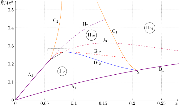
Figure 11: Moduli space of configurations with mode numbers $n_{1}=1$, $n_{2}=2$, shown in the $(\alpha,\tilde{E})$ plane. Regions of the space are named by roman numbers $\mathrm{I}$-$\mathrm{III}$, while lines are assigned Latin letters $\mathrm{A}$-$\mathrm{J}$. Special points have labels $\mathrm{X}$-$\mathrm{Z}$. The dotted area is magnified in Fig. 12. The moduli spaces of higher mode numbers look very similar, cf. Fig. 14.

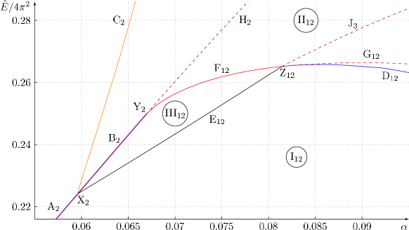
Figure 12: Magnification of the dotted area in Fig. 11

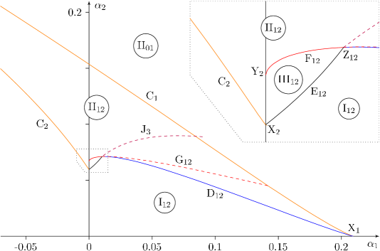
Figure 13: The same moduli space as in Fig. 11, shown in the $(\alpha_{1},\alpha_{2})$ plane. The lines $\mathrm{A}_{1}$, $\mathrm{B}_{1}$, $\mathrm{A}_{2}$ and $\mathrm{H}_{2}$ lie on the axes.

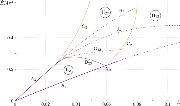
Figure 14: Moduli space of configurations with mode numbers $n_{1}=2$, $n_{2}=3$, shown in the $(\alpha,\tilde{E})$ plane. The dotted area is magnified in Fig. 15. Structurally, the moduli spaces of higher pairs of mode numbers like this one are very similar to the case $n_{1}=1$, $n_{2}=2$ shown in Fig. 11. One can already see that the part of the space shown here is connected to the part shown in Fig. 11.

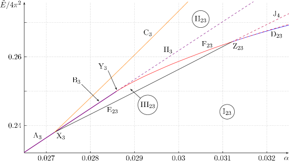
Figure 15: Magnification of the dotted area in Fig. 14

To begin with, the moduli spaces of configurations with two consecutive mode numbers can be divided into several regions, as is shown in Fig. 11,12,13,14,15 for the cases of $n_{1}=1$, $n_{2}=2$ and $n_{1}=2$, $n_{2}=3$. Solutions in each region and on each line separating the regions share certain characteristics. In the following sections, the different regions, lines and points of the moduli space will be discussed in detail and examples will be given. For simplicity, only non-negative mode numbers $n_{i}\geq 0$ are considered, which correspond to cuts that lie to the right of the imaginary line. The discussion for negative mode numbers is completely analogous. The two cuts are named “cut one” and “cut two”. Unless otherwise stated, the mode number $n_{1}$ of cut one is smaller than the one of cut two, $n_{2}=n_{1}+1$.

In all figures that show cut contours or densities, cut one has blue colour (thick lines), while cut two has red colour (thin lines). Plots of cut contours in the complex plane always have an aspect ratio of $1:1$. In all density plots, the density is shown versus the distance from the cut’s centre, measured along the cut’s contour.

5.2 Regions

The moduli space of configurations with two given consecutive mode numbers can be divided into three regions. Configurations in each region share certain characteristics: In region $\mathrm{I}$, the two cuts are disjoint; in region $\mathrm{II}$, the cuts join with each other and form a condensate with four tails; in region $\mathrm{III}$, the two cuts are disjoint but require a third, closed cut and a condensate for stability. In the following paragraphs, the characteristics of the different regions are described in more detail and example solutions are shown.

Region $\mathrm{I}_{n,n+1}$: Two Disjoint Cuts.

In this region, the contours of the two cuts with mode numbers $n$ and $n+1$ are disjoint, and the cut with mode number $n+1$ lies further left (closer to the origin) than the one with mode number $n$. The absolute density is bounded above by $1$ everywhere on both cuts. An example is shown in Fig. 16. When the filling of one of the cut increases, this cut attracts the other one, as can be seen in Fig. 17,18.

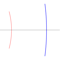
(a) Cut contours

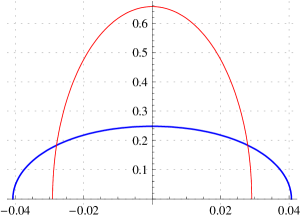
(b) Absolute densities along the cuts vs. distance from the cuts’ centres (measured along the contour)

Figure 16: Cut contours and absolute densities of an example solution in region $\mathrm{I}_{12}$ (see Fig. 11). The fillings are $\alpha_{1}=0.016$ (blue/thick, $n_{1}=1$) and $\alpha_{2}=0.03$ (red/thin, $n_{2}=2$).

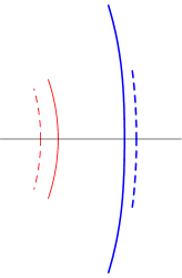
(a) Cut contours

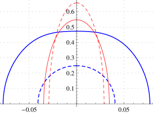
(b) Absolute densities along the cuts vs. distance from the cuts’ centres (measured along the contour)

Figure 17: Another configuration in region $\mathrm{I}_{12}$. The cut contours and densities of Fig. 16 are shown with dashed lines. Cut one has a larger filling than in Fig. 16 and attracts cut two ($\alpha_{1}=0.06$, $\alpha_{2}=0.03$).

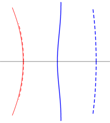
(a) Cut contours

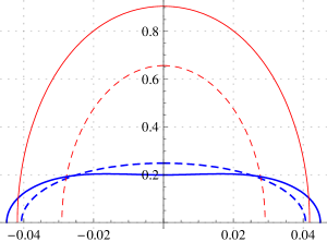
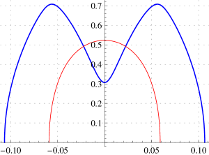
(b) Absolute densities along the cuts vs. distance from the cuts’ centres (measured along the contour)

Figure 18: A third configuration in region $\mathrm{I}_{12}$. The cut contours and densities of Fig. 16 are shown with dashed lines. Cut two has a larger filling than in Fig. 16 and attracts cut one ($\alpha_{1}=0.016$, $\alpha_{2}=0.06$).

Region $\mathrm{II}_{n,n+1}$: Condensate with Four Tails.

In this region, the standard contours of the two cuts bend towards and cross each other. An example is shown in Fig. 19.

(a) Cut contours

(b) Absolute densities along the cuts vs. distance from the cuts’ centres (measured along the contour)

Figure 19: Standard cut contours and absolute densities of an example configuration in region $\mathrm{II}_{12}$ (see Fig. 11). The fillings fractions are $\alpha_{1}=0.11$ (blue/thick, $n_{1}=1$) and $\alpha_{2}=0.05$ (red/thin, $n_{2}=2$). This particular configuration lies below line $\mathrm{G}_{12}$ in the $(\alpha,\tilde{E})$ plane. The physical version of the configuration has a condensate and is shown in Fig. 20.

As explained below (2.14), the sum of the densities at the two common points of the standard contours equals $-i$ (since the difference of the mode numbers is $n_{1}-n_{2}=-1$) and solutions in this region allow for straight condensate cuts with constant density $\rho_{\mathrm{c}}(x)=-i$ between the two common points of the cuts. The condensate-cut version of the configuration in Fig. 19 is shown in Fig. 20.

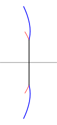
(a) Cut contours

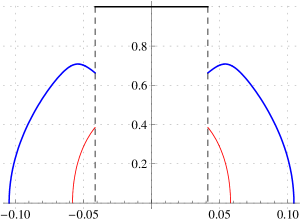
(b) Absolute densities along the cuts vs. distance from the cuts’ centres (measured along the condensate and the cuts’ contour)

Figure 20: Physical version of the configuration shown in Fig. 19. The two common points of the standard contours are connected by a condensate.

Beyond the two common points, the remaining parts of the standard cut contours form four tails that are attached to the ends of the condensate. The tails of cut two (with mode number $n+1$) lie further left than the ones of cut one (with mode number $n$).

Whenever a particular solution $p$ allows for a condensate cut, it will be assumed that the configuration with the condensate cut is the physical version of the solution. This assumption may not seem very motivated at the moment, but will become more justified during the subsequent discussion. A first sign of its verity is the fact that there is no well-defined direction on standard cut contours that cross each other. This can be seen as follows: According to (2.12), the density $\rho$ on a standard cut contour is proportional to the difference between the limiting values of $p(x)$ on either side of the cut contour: $\rho(x)\sim p(x+\epsilon)-p(x-\epsilon)$. When a standard cut contour crosses another standard cut contour, the value of $p(x\pm\epsilon)$ on either side of the contour changes to $-p(x\pm\epsilon)+2\pi n$, where $n$ is the mode number of the cut that is traversed; this follows from the Bethe equations (1.1). Hence the density $\rho$ on the contour switches its sign, and in order that the corresponding root density $\rho(x)\,\mathrm{d}x$ stays positive, the direction on the contour must change as well. However a unique direction on each contour was assumed in the derivation of the spectral curve and quasi-momentum in Sec. 2.3. This argument makes it seem very unlikely that configurations with crossing standard cut contours can be realised as limits of Bethe root distributions.

As indicated by the dashed lines in Fig. 11,12,13,14,15, region $\mathrm{II}_{n,n+1}$ can be further subdivided. Between the lines $\mathrm{D}_{n,n+1}$, $\mathrm{G}_{n,n+1}$ and $\mathrm{C}_{n}$, the standard cut contours have the usual form, as in Fig. 19: Neither do they encircle the origin, nor do they extend to infinity. In contrast, beyond line $\mathrm{G}_{n,n+1}$ the standard contour of cut one encircles the origin, as in the example in Fig. 21.

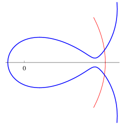
(a) Cut contours

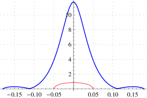
(b) Absolute densities along the cuts vs. distance from the cuts’ centres (measured along the contour)

Figure 21: An example configuration in region $\mathrm{II}_{12}$ beyond line $\mathrm{G}_{12}$ (see Fig. 11). The filling fractions are $\alpha_{1}=0.032$ (blue/thick, $n_{1}=1$) and $\alpha_{2}=0.07$ (red/thin, $n_{2}=2$). The physical version of this solution has a condensate cut and is shown in Fig. 22.

Moving a contour with filling $\alpha_{1}$ past the pole at the origin changes its filling to $\alpha_{1}^{\prime}=\alpha_{1}+1$; this follows from the expression of the filling fraction as a contour integral (2.23), the residue theorem and the fact that the residue at $x=0$ switches its sign as the contour moves past it. As a result, the absolute density on the standard contour typically exceeds unity at its centre, as in Fig. 21. This and the fact that the pole at the origin has the wrong sign in this configuration are strong indications that the physical realisation of such a solution is the one with a condensate cut, as in Fig. 22.

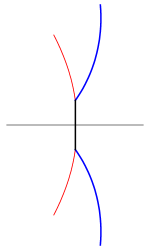
(a) Cut contours

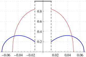
(b) Absolute densities along the cuts vs. distance from the cuts’ centres (measured along the condensate and the cuts’ contours)

Figure 22: Physical version of the solution shown in Fig. 21. The part of cut one that encircles the origin is hidden in the condensate cut.

Physically, there is no qualitative difference between configurations on either side of line $\mathrm{G}_{n,n+1}$, as their physical versions always contain a condensate cut and thus do not see the central part of the standard cut contours. Note that below line $\mathrm{G}_{n,n+1}$, as in the example in Fig. 19, the absolute density does not exceed unity on the standard cut contours. Hence the stability criterion (2.29) is obeyed by the standard contours and no condensate is necessary to fulfil (2.27). Yet a condensate version of the configuration is possible. Beyond line $\mathrm{G}_{n,n+1}$ a condensate is necessary for stability, and for continuity reasons one would assume that also below line $\mathrm{G}_{n,n+1}$ the physical version is the one with a condensate cut. This is another sign in favour of the assumption that if a condensate cut is possible, it is also realised physically.

The other dashed lines $\mathrm{H}_{n,n+1}$ and $\mathrm{J}_{n,n+1}$ that further subdivide region $\mathrm{II}_{n,n+1}$ are discussed in Sec. 5.3 below.

Region $\mathrm{III}_{n,n+1}$: Two Disjoint Cuts, One with a Condensate.

In this region, the contours of the two cuts are disjoint as in region $\mathrm{I}_{n,n+1}$, but the absolute density exceeds unity at the centre of cut two, i.e. the stability condition (2.29) is violated. An example configuration is shown in Fig. 23.

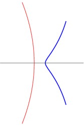
(a) Cut contours

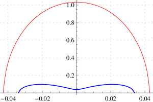
(b) Absolute densities along the cuts vs. distance from the cuts’ centres (measured along the contour)

Figure 23: An example solution in region $\mathrm{III}_{12}$ (see Fig. 11). The fillings are $\alpha_{1}=0.0038$ (blue/thick, $n_{1}=1$) and $\alpha_{2}=0.07$ (red/thin, $n_{2}=2$). The absolute density exceeds unity at the centre of cut two, hence the stability criterion (2.29) is violated. The physical version of the configuration involves a condensate cut and is shown in Fig. 24.

Configurations in this region are still physical, because the same discussion as in Sec. 3.5 is applicable: A third, closed cut can be added in order to form a condensate at the centre of cut two. Since the absolute density at the centre of cut two exceeds unity, the excitation point with mode number $n+2$ has already passed through the contour of cut two and changed its mode number to $n$. The closed cut originates and ends at this excitation point. The resulting physical version of such a configuration is shown in Fig. 24.

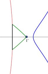
(a) Central part of the cut contours

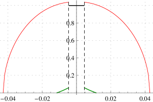
(b) Absolute density along cut two, the closed cut and the condensate vs. distance from the condensate’s centre (measured along the contour)

Figure 24: Physical version of the configuration shown in Fig. 23. A third, closed cut forms a condensate with cut one, as in the one-cut case discussed in Sec. 3.5. The closed cut starts and ends at the excitation point $1^{\prime}$, which passed through cut two as the density at the centre of cut two reached unity.

5.3 Lines

In the following paragraphs, the features of configurations on the various lines shown in Fig. 11,12,13,14,15 are presented and appropriate examples are given.

Line $\mathrm{A}_{n}$: Only One Cut.

This line represents configurations where only the cut with mode number $n$ is present and has a filling $\alpha<\alpha_{\mathrm{cond}}$ (cf. Tab. 1), such that the absolute density at the cut’s centre always stays below unity. Among all configurations with mode numbers $n$ and $n+1$ and given total filling, the state on this line is the one with the lowest energy. Adding a second cut with higher mode number while keeping the total filling constant obviously increases the energy. Conversely, adding a second cut with lower mode number while keeping the total filling constant decreases the total energy.

Line $\mathrm{B}_{n}$: Only One Cut with a Condensate.

This line is the continuation of line $\mathrm{A}_{n}$. Solutions on this line have only one cut with mode number $n$ which has a filling $\alpha_{\mathrm{cond}}<\alpha<\alpha_{\mathrm{crit}}$ and were discussed in Sec. 3. The absolute density at the centre of the cut’s standard contour exceeds unity; hence a second, closed cut that starts and ends at the excitation $(n-1)^{\prime}$ and forms a condensate with the central part of the cut is required for stability, as in the second example in Fig. 8.

Line $\mathrm{C}_{n}$: Condensate with Two Tails.

Line $\mathrm{C}_{n}$ separates region $\mathrm{II}_{n,n+1}$ from region $\mathrm{II}_{n-1,n}$, which both consist of solutions with a condensate cut. Solutions on line $\mathrm{C}_{n}$ consist of a larger cut (cut one) with mode number $n$ and a smaller cut (cut two), whose end points lie exactly on the standard contour of the larger cut. Therefore, the physical version of such a configuration consists of a condensate with one tail at each of its ends; the smaller cut is completely hidden in the condensate. Since the density of cut two at the cut’s end points vanishes, the density of cut one at these points must equal $-i$, as explained below (2.14). Consequently, also the direction of cut one at these points is purely imaginary, i.e. vertical. Hence, the cut contour of the condensate version of this configuration and the density along it are smooth. Solutions on this line were investigated by Sutherland in [8], refer to Figure 2 in that reference for a picture of the absolute density on the condensate and the tails.

A series of configurations in which the branch points of cut two pass the contour of cut one is shown in Fig. 25.

(a) 0.12

(b) 0.13

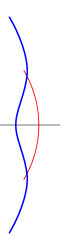
(c) 0.14

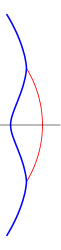
(d) 0.1487

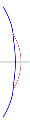
(e) 0.1487

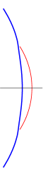
(f) 0.155

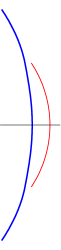
(g) 0.165

Figure 25: A Series of configurations that passes through line $\mathrm{C}_{1}$ in Fig. 11. At all points of the series, the filling fraction of the small cut equals $\alpha_{2}=0.04$. The filling fraction $\alpha_{1}$ of the large cut is indicated below each plot. Configurations (d) and (e) are the same in terms of mode numbers, fillings and branch points, but, as explained in the main text, this solution allows for two different contours for cut one. All solutions have a condensate in their physical version as displayed in Fig. 28.

The sequence passes line $\mathrm{C}_{1}$ from left to right in Fig. 11. During the series, the filling fraction of cut two stays constant, while the filling fraction of cut one increases. At the beginning, the configuration is in region $\mathrm{II}_{12}$: The branch points of cut two lie to the left of cut one, and the mode number of cut two is $n_{2}=2$, while the mode number of cut one is $n_{1}=1$ (Fig. 25a,25b,25c). While the filling fraction of cut one increases, cut two gets attracted by it and moves further right. During this process, the cuts increasingly bend towards each other and both become longer. At a certain value of the large cut’s filling, the end points of the small cut lie exactly on the large cut’s contour, the configuration has arrived at line $\mathrm{C}_{1}$ (Fig. 25d). One can see that the contour of cut one is indeed vertical at the end points of cut two. The filling of cut two stays constant during the series, but its length increases, hence the absolute density along its contour decreases.

When the filling of cut one increases further, the small cut’s branch points move on to its other side and the configuration reaches region $\mathrm{II}_{n-1,n}$ (Fig. 25f,25g). While the end points of cut two pass the large cut, multiple quantities change: According to (4.13), the mode number of a cut is $n_{i}=\pi p(x_{*})$, where $x_{*}$ is a branch point of the cut. Across a cut with mode number $n_{1}$, $p$ switches sign and shifts by $2\pi n_{1}$ (2.11). Therefore, a cut with mode number $n_{2}$ whose branch points pass another cut with mode number $n_{1}$ changes its mode number to $n_{2}^{\prime}=-n_{2}+2n_{1}$. Specifically, if $n_{2}=n_{1}+1$, as in the series in Fig. 25, then $n_{2}^{\prime}=n_{1}-1$. Further, while cut two passes through the contour of cut one, the sign of the density (2.12) along cut two changes, as shown above in the discussion of region $\mathrm{II}_{n,n+1}$. This does not affect the density of roots along the cut, but it switches the sign of the filling: $\alpha_{2}\rightarrow\alpha_{2}^{\prime}=-\alpha_{2}$. Thirdly, the contour of cut one and its filling change by a finite amount when cut two passes. The filling changes from $\alpha_{1}$ to $\alpha_{1}^{\prime}=\alpha_{1}+2\alpha_{2}$, which is consistent with the fact that the total filling $\alpha_{1}+\alpha_{2}$, as a coefficient of the expansion of $p$ at infinity (2.17), must vary continuously during the series. Also the total momentum $m=n_{1}\alpha_{1}+n_{2}\alpha_{2}$ varies continuously during the transition from region $\mathrm{II}_{n,n+1}$ to region $\mathrm{II}_{n-1,n}$.

For a qualitative picture of the densities on the cuts in the series, refer to Fig. 19b,26b. As a consequence of the change in the contour and the filling of cut one, in all solutions beyond line $\mathrm{C}_{n}$ (right of $\mathrm{C}_{n}$ in the $(\alpha,\tilde{E})$ plane) the absolute density exceeds unity at the centre of cut one’s standard contour. The standard contour of cut two is disjoint from cut one, as in Fig. 26.

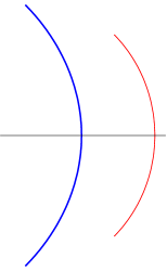
(a) Cut contours

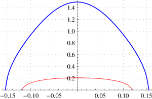
(b) Absolute densities along the cuts vs. distance from the cuts’ centres (measured along the contour)

Figure 26: Standard cut contours and absolute densities of an example solution in region $\mathrm{II}_{n-1,n}$, beyond line $\mathrm{C}_{1}$ (see Fig. 11). The fillings are $\alpha_{1}=0.25$ (blue/thick, $n_{1}=1$) and $\alpha_{2}=0.04$ (red/thin, $n_{2}=0$). The absolute density exceeds unity at the centre of cut one, hence this configuration is unstable. The physical, stable form of this solution is shown in Fig. 27.

In this form, the configuration does not allow for a condensate cut and is therefore unstable. However, there still is a stable version of such solutions: As discussed below (2.13), there are three possible starting directions for a cut at each branch point. Choosing a different direction for cut two, this cut’s contour can be made to cross the contour of the first cut, and the unphysical density at the first cut’s centre becomes hidden in a condensate. For the solution in Fig. 26, his type of configuration is shown in Fig. 27.

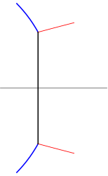
(a) Cut contours

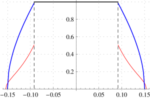
(b) Absolute densities along the cuts vs. distance from the cuts’ centres (measured along the condensate and the cuts’ contours)

Figure 27: Physical version of the solution shown in Fig. 26. Cut two (red/thin) has a different starting direction than in Fig. 26 and hence a different contour, which allows for the formation of a condensate cut that hides the central part of cut one (blue/thick) and renders the configuration stable.

These condensate-cut versions of the solutions beyond line $\mathrm{C}_{n}$ not only cure the instability at the centre of cut one, they also allow for a smooth transition from configurations on line $\mathrm{C}_{n}$ to solutions beyond line $\mathrm{C}_{n}$. This can be seen in Fig. 28, where the physical version of the series of Fig. 25 is displayed.

(a) 0.12

(b) 0.13

(c) 0.14

(d) 0.1487

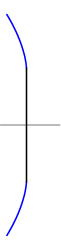
(e) 0.1487

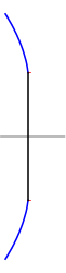
(f) 0.155

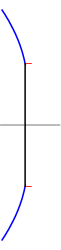
(g) 0.165

Figure 28: Physical version of the series of solutions in Fig. 25. The configurations LABEL:sub@fig:12_lineD_series_cond_f and LABEL:sub@fig:12_lineD_series_cond_g show the physical, smooth continuation of the series beyond line $\mathrm{C}_{1}$.

The changes that occur when the branch points of cut two pass the contour of cut one imply that configurations on line $\mathrm{C}_{n}$ have an ambiguity in the mode number of cut two and in the standard contour of cut one. This can be seen in the example in Fig. 25d,25e. In the limit where cut two approaches cut one from the left, the mode number of cut two is $n_{2}=n_{1}+1$, and the contour of cut one is bent to the left. In the other limit, where cut two approaches cut one from the right, the mode number of cut two is $n_{2}=n_{1}-1$, and cut one is bent to the right. The fillings of the cuts behave accordingly, as described in the discussion of the series above. On line $\mathrm{C}_{n}$, the contour of cut one is unique between its end points and the branch points of cut two. The fact that the contour is ambiguous between the two branch points of cut two is consistent with the fact that the expansion of $p$ has a square root term at the branch points $x_{*}$ (cf. (2.13)):

$$p(x_{*}+\varepsilon)=p(x_{*})+A\sqrt{\varepsilon}+\mathcal{O}(\varepsilon)\,,$$ (5.1)

because this results in the expansion of the density (as follows from (2.12))

$$\rho_{1}(x_{*}+\varepsilon)=\frac{1}{\pi i}\left(p(x_{*}+\varepsilon)-\pi n_{1}\right)=i\left(n_{1}-n_{2}-\pi A\sqrt{\varepsilon}\right)+\mathcal{O}(\varepsilon)\,,$$ (5.2)

which implies that the solution of the differential equation $\rho_{1}(x)\mathrm{d}x\in\mathbb{R}$ has an ambiguous second derivative at the branch points $x_{\pm}$ and hence there are two choices for the continuation of the contour beyond the branch points $x_{*}$. However, this ambiguity has no physical significance, as the physical configuration with the condensate is non-ambiguous.

Line $\mathrm{D}_{n,n+1}$: Two Tangential Cuts.

This line separates region $\mathrm{I}_{n,n+1}$ from region $\mathrm{II}_{n,n+1}$. The two cut contours of configurations on this line bend towards each other and touch each other in one point on the real axis. At the common point of the contours, the sum of the two densities equals $-i$. An example is shown in Fig. 29. Beyond this line, the formation of condensate cuts begins.

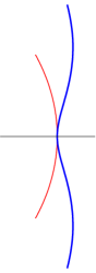
(a) Cut contours

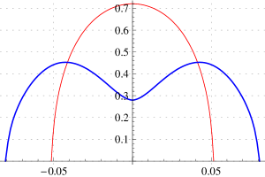
(b) Absolute densities along the cuts vs. distance from the cuts’ centres (measured along the contour)

Figure 29: An example configuration on line $\mathrm{D}_{12}$. The fillings are $\alpha_{1}=0.05833$ (blue/thick, $n_{1}=1$) and $\alpha_{2}=0.06$ (red/thin, $n_{2}=2$). The cuts touch at one point on the real axis, where the sum of their densities equals $-i$.

Line $\mathrm{E}_{n,n+1}$: Cut Two Violating Stability.

This line can be reached from region $\mathrm{I}_{n,n+1}$ by increasing the filling of cut two while keeping the filling of cut one small, such that the two cuts stay disjoint. Line $\mathrm{E}_{n,n+1}$ is reached when the absolute density at the centre of cut one reaches unity. At this point, the excitation with mode number $n+2$ collides with the contour of cut two from the left. Further increasing the filling of cut two makes the excitation pass to the right of the contour and change its mode number to $n$. The absolute density on the standard contour of cut two now exceeds unity and a third, closed cut is required for stability; the configuration has reached region $\mathrm{III}_{n,n+1}$ (cf. Fig. 24).

Line $\mathrm{F}_{n,n+1}$: Two Disjoint Cuts and a Cusp on Cut One.

This line separates region $\mathrm{III}_{n,n+1}$, where the standard cut contours of the two cuts are disjoint, from solutions in region $\mathrm{II}_{n,n+1}$, in which cut one encircles the origin and consequently crosses the contour of cut two. A sequence of configurations that passes line $\mathrm{F}_{12}$ from region $\mathrm{III}_{12}$ to region $\mathrm{II}_{12}$ is shown in Fig. 30.

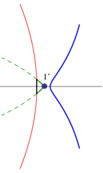
(a) 0.0703

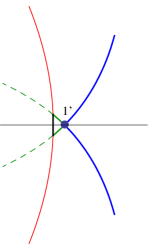
(b) 0.07042

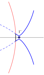
(c) 0.0705

Figure 30: A sequence of configurations that passes line $\mathrm{F}_{12}$. Cut one (blue/thick) has mode number $n_{1}=1$ and constant filling $\alpha_{1}=0.005$, cut two (red/thin) has mode number $n_{2}=2$ and its filling $\alpha_{2}$ is indicated below each subfigure. The excitation with mode number $1$ is shown and carries a closed cut (green/thick) which forms a condensate cut at the centre of cut two. Configuration (a) lies in region $\mathrm{III}_{12}$, configuration (b) lies on line $\mathrm{F}_{12}$ and configuration (c) lies in region $\mathrm{II}_{12}$. The dashed contours all close around the origin. The energy increases during the sequence.

The transition happens when the excitation $n^{\prime}$, which carries a closed loop that forms a condensate with cut two, reaches the contour of cut one. At this point, the contour of the closed loop merges with cut one, whose standard contour encircles the origin afterwards. The transition point is marked by line $\mathrm{F}_{n,n+1}$. On this line, the density (2.9) on cut one decreases to zero at the merging point $x_{0}$, as $p(x_{0})=\pi n$. Around this point, the density expands to $\rho_{1}(x_{0}+\varepsilon)\mathrm{d}\varepsilon\sim\varepsilon^{2}$, which implies that the contour has a cusp with opening angle $90^{\circ}$.

Line $\mathrm{G}_{n,n+1}$: Condensate with Tails and a Virtual Cusp.

This line in region $\mathrm{II}_{n,n+1}$ separates solutions in which the standard contour of cut one closes on the right side of the origin from solutions in which it encircles the origin (cf. Fig. 19,21). The qualitative change that happens to cut one’s contour when crossing this line is the same as on line $\mathrm{F}_{n,n+1}$: The excitation point $n^{\prime}$ collides with the standard contour, making the density decay to zero at its centre. Unlike on line $\mathrm{F}_{n,n+1}$, here the process is less significant because the central part of cut one is hidden in the condensate. An example configuration that lies on line $\mathrm{G}_{12}$ is displayed in Fig. 31.

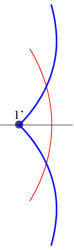
(a) Cut contours

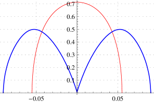
(b) Absolute densities along the cuts vs. distance from the cuts’ centres

Figure 31: An example configuration on line $\mathrm{G}_{12}$. The fillings are $\alpha_{1}=0.0635$ (blue/thick, $n_{1}=1$) and $\alpha_{2}=0.064$ (red/thin, $n_{2}=2$). The excitation with mode number $1$ is shown and lies on the standard contour of cut one, which implies that the density (2.12) decays to zero at that point.

Line $\mathrm{H}_{n}$: One Cut with Vanishing Virtual Filling.

On this line, the filling $\alpha_{1}$ of cut one (with mode number $n-1$) vanishes. However, as shown above in the discussion of region $\mathrm{II}_{n,n+1}$, the standard contour of cut one encircles the origin and the filling on this contour equals one. Since most of cut one is hidden in the condensate cut, the vanishing filling of the physical cut contour does not have any further implications for the physical configuration. An example is given in Fig. 32. Because the filling of cut one vanishes, there is a one-cut solution with the same mode numbers and fillings for each solution on this line. These one-cut solutions are of the type shown in Fig. 8c and have a higher total energy than the corresponding solutions on line $\mathrm{H}_{n}$. Refer to the discussion of point $\mathrm{Y}_{n}$ below for more details on the relation between these two types of solutions.

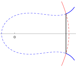
(a) Physical version of the cut contours. Dashed lines show the hidden part of the standard contours.

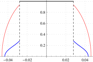
(b) Absolute densities along the condensate and the tails vs. distance from the condensate’s centre (measured along the contour).

Figure 32: An example configuration on line $\mathrm{H}_{2}$. The fillings are $\alpha_{1}=0$ (blue/thick, $n_{1}=1$) and $\alpha_{2}=0.085$ (red/thin, $n_{2}=2$). The parts of the standard contours that are hidden in the condensate cut are shown as dashed lines. Since the standard contour of cut one encircles the origin, the integral of the absolute density along it is not zero, but unity.

Line $\mathrm{J}_{n}$: Excitation $n$ Collides with the Condensate.

These lines mark all configurations where the excitation point with mode number $n$ is located on the condensate cut. When line $\mathrm{J}_{n}$ gets traversed, the excitation point with mode number $n$ collides with the condensate from the left and passes to the right (for positive mode numbers), thereby changing its mode number to $n-2$. But unlike an excitation point passing a standard cut, this process does not create an additional, closed cut (as on line $\mathrm{E}_{n,n+1}$); in fact, the passage of the excitation point has no effect on the configuration at all.

5.4 Special Points

As a result of the discussion of the various regions and lines in the previous sections, three types of special points emerge, labelled by $\mathrm{X}_{n}$, $\mathrm{Y}_{n}$ and $\mathrm{Z}_{n,n+1}$ in the Fig. 11,12,13,14,15. These points will be discussed in the following.

Point $\mathrm{X}_{n}$: Excitation Point Meets Single Cut.

The points $\mathrm{X}_{n}$ mark the one-cut solutions with mode number $n$ whose absolute density equals unity at the cut’s centre, which means that the excitation point with mode number $n+1$ is located on the cut’s contour. The filling fractions of these solutions for $n\leq 10$ can be found in Tab. 1. The point $\mathrm{X}_{n}$ connects line $\mathrm{A}_{n}$, on which the absolute density on the single cut’s centre falls below unity, with line $\mathrm{B}_{n}$, on which the absolute density at the centre of the standard contour exceeds unity and a condensate begins to form with the help of a second, closed cut. Also the lines $\mathrm{C}_{n}$, $\mathrm{D}_{n,n+1}$ and $\mathrm{E}_{n-1,n}$ begin at the point $\mathrm{X}_{n}$ (the last one only if $n>1$). Among all configurations on line $\mathrm{A}_{n}$, the one at this point has the highest energy (cf. Tab. 1).

Point $\mathrm{Y}_{n}$: The Two Excitation Points with the Same Mode Number Collide.

Point $\mathrm{Y}_{n}$ marks the end of line $\mathrm{B}_{n}$ and thus represents a one-cut solution with a condensate. On line $\mathrm{B}_{n}$, the two excitation points $(n-1)^{\prime}$ and $(n-1)$ both lie on the real line, as in Fig. 8b. At the point $\mathrm{Y}_{n}$, these two excitation points collide. Analytically continuing line $\mathrm{B}_{n}$ beyond point $\mathrm{Y}_{n}$ lets the branch points diverge into the complex plane and leads to one-cut solutions of the type shown in Fig. 8c. This analytic continuation of line $\mathrm{B}_{n}$ shall be called line $\mathrm{B}_{n}^{\prime}$. As discussed in Sec. 3.5, solutions on this line are limiting cases of three-cut solutions. Hence line $\mathrm{B}_{n}^{\prime}$ is not part of the moduli space of two-cut solutions (or of its boundary).

The only way to continue beyond point $\mathrm{Y}_{n}$ while staying in the regime of consecutive mode numbers is to enter either region $\mathrm{II}_{n-1,n}$ or region $\mathrm{III}_{n-1,n}$. In both cases, the excitation points $(n-1)^{\prime}$ and $(n-1)$ separate again. The former stays on the real line, while the latter splits into two square root branch points that diverge into the complex plane. Upon entering region $\mathrm{III}_{n-1,n}$, the excitation point $(n-1)^{\prime}$ continues to carry a closed cut as on line $\mathrm{B}_{n}$ while the new branch points form the ends of a second standard cut, as in Fig. 30a. When the configuration enters region $\mathrm{II}_{n-1,n}$, the afore closed cut opens up at its cusp and becomes a standard cut that ends on the new pair of branch points, as in Fig. 30c. Either way, a second standard cut emerges, which can have a positive, negative or vanishing filling. Configurations with vanishing filling belong to line $\mathrm{H}_{n}$ and lie in region $\mathrm{II}_{n-1,n}$. Since the closed cut in the solutions on line $\mathrm{B}_{n}$ also has zero filling, line $\mathrm{H}_{n}$ seems to be the most natural continuation of line $\mathrm{B}_{n}$.

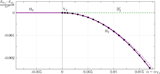
Figure 33: Deviation of the energy on line $\mathrm{H}_{2}$ from the energy on line $\mathrm{B}_{2}^{\prime}$ (green/dashed), which is the analytic continuation of line $\mathrm{B}_{2}$ (purple/solid). Shown are the energies of numerically obtained solutions on line $\mathrm{H}_{2}$ (black dots), the corresponding function $\tilde{E}_{\mathrm{H}_{n}}-\tilde{E}_{\mathrm{B}_{n}^{\prime}}$ (purple/solid) and the quadratic term of (5.3) (purple/dashed). The energy deviation is measured between solutions with the same total filling $\alpha$ and shows that a second order phase transition occurs upon the passage from line $\mathrm{B}_{n}$ to line $\mathrm{H}_{n}$.

As noted at the end of Sec. 3, solutions on line $\mathrm{B}_{n}^{\prime}$ can be transformed into the corresponding solutions on line $\mathrm{H_{n}}$ by separating the two segments of the closed cut in Fig. 8c. In doing so, the two excitation points in the complex plane split into two square-root branch points each, which results in a three cut solution. The filling of the third, vertical cut can then be decreased to zero while the filling of the second cut increases to zero, such that the total filling fraction $\alpha$ stays constant. During this process, the energy decreases. Comparing the energy of solutions on line $\mathrm{H}_{n}$ to the energy of the corresponding one-cut solutions on line $\mathrm{B}_{n}^{\prime}$ (Fig. 33) shows that a second order phase transition occurs as a configuration follows line $\mathrm{B}_{n}$ and continues on line $\mathrm{H}_{n}$. For example, the deviation of the energy on line $\mathrm{H}_{n}$ from the energy on line $\mathrm{B}_{n}^{\prime}$ has the following expansion in the total filling at point $\mathrm{Y}_{n}$:

$$(\tilde{E}_{\mathrm{H}_{n}}-\tilde{E}_{\mathrm{B}_{n}^{\prime}})(\alpha)=-8\pi^{2}n^{2}(\alpha-\alpha_{\mathrm{Y}_{n}})^{2}+\mathcal{O}((\alpha-\alpha_{\mathrm{Y}_{n}})^{3})\,.$$ (5.3)

The prefactor of the quadratic deviation, including its dependency on $n$, has been guessed on the basis of numerical data which, for the first few values of $n$, matches this form with high accuracy. On a technical level, this phase transition is related to the one discussed by Douglas and Kazakov in [32]: It involves a transition between the same classes of algebraic curves and it is also related to a density threshold, see App. B for a technical review. The authors study the large-$N$ limit of the partition function of continuous pure Yang-Mills theory on the two-sphere and find a phase transition with respect to the area of the sphere.

Point $\mathrm{Z}_{n,n+1}$: Cusp on Cut One Meets Cut Two.

At this point, the lines $\mathrm{F}_{n,n+1}$ and $\mathrm{G}_{n,n+1}$ meet: Cut one has a cusp at the centre of its contour whose tip lies on the contour of cut two. Since the tip of the cusp marks the excitation point with mode number $n+2$, this implies that the absolute density of cut two at this point equals unity and that lines $\mathrm{E}_{n,n+1}$ and $\mathrm{J}_{n+2}$ also end on point $\mathrm{Z}_{n,n+1}$. The two cuts touch each other only in one point, thus also line $\mathrm{D}_{n,n+1}$ ends here.

5.5 Global Structure of the Moduli Space

As a consequence of the discussion about the lines $\mathrm{C}_{n}$ in Sec. 5.3, all moduli spaces of two consecutive mode numbers are analytically connected through the lines $\mathrm{C}_{n}$. Pictures of the resulting global space are shown in Fig. 34,35. In the latter, also the lines of unstable one-cut solutions $\mathrm{B}_{n}^{\prime}$ are shown for comparison, while in the former these lines are the same as the lines $\mathrm{H}_{n}$. In particular, the global connectedness of the space shows that mode numbers lose their intuitive meaning at large filling fractions: A small change in the number of excitations (filling fractions) can alter the mode numbers, hence they can no longer be interpreted as the number of periods of a coherent state on the spin chain.

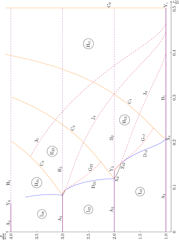
Figure 34: Global structure of the moduli space for consecutive mode numbers, shown in the $(P,P/\alpha)$ plane.

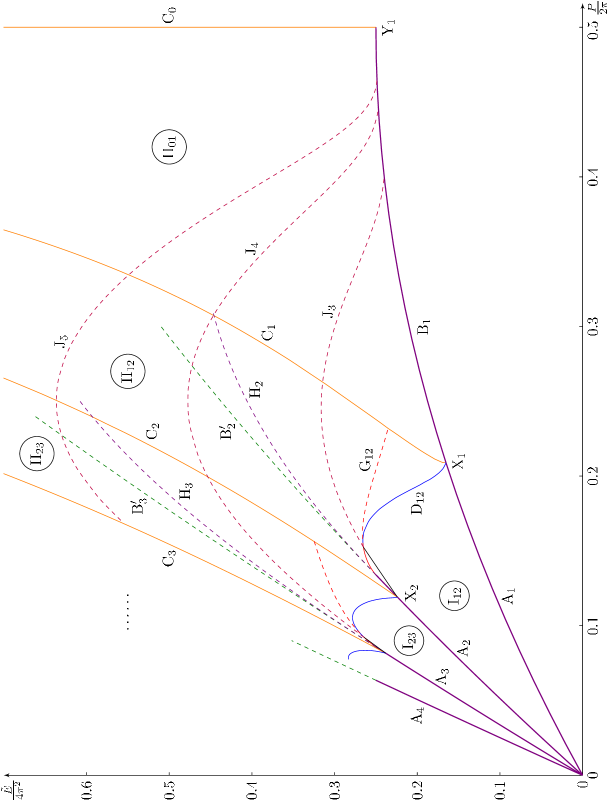
Figure 35: Global structure of the moduli space for consecutive mode numbers, shown in the $(P,\tilde{E})$ plane.

Note that the case $n_{1}=0$ (cut one), $n_{2}=1$ (cut two) qualitatively differs from the other cases with consecutive mode numbers. The excitation point $n_{*}=0$ always lies at $x=\infty$ and hence cannot be excited, only the excitation point $n_{*}=0^{\prime}$ can. Consequently, line $\mathrm{B}_{1}$ cannot be crossed, and cut one always has a negative filling and its standard contour winds around the origin. That means that solutions with mode numbers $n_{1}=0$, $n_{2}=1$ always have a condensate and regions $\mathrm{I}_{01}$ and $\mathrm{III}_{01}$ do not exist.

The one-cut lines $\mathrm{A}_{n}$ and $\mathrm{B}_{n}$, $n>1$, form branch cuts of the global moduli space; across them, the derivatives of physical quantities such as the energy and the momentum are discontinuous. The points $\mathrm{Y}_{n}$, $n>1$ are the corresponding branch points.

As mentioned at the end of Sec. 3.5, at point $\mathrm{Y}_{1}$ the excitation point $n_{*}=0^{\prime}$ reaches $x=\infty$. At that point, the filling fraction of cut two equals $\alpha_{2}=1/2$ and cut one extends along the whole imaginary line while the branch points of cut two are $x_{\pm}=\pm i/2\pi$. The absolute density of this solution is shown in Fig. 36.

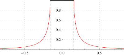
Figure 36: Absolute density along the condensate and the two tails of the solution at point $\mathrm{Y}_{1}$. Cut one ($n_{1}=0$, $\alpha_{1}=0$, red/thin) extends along the whole imaginary line, while the branch points of cut two ($n_{2}=1$, $\alpha_{2}=1/2$) are $x_{\pm}=\pm i/2\pi$. The absolute density on the tails falls off as $1/|x|$.

When the filling of cut one gets reduced to finite negative values while $\alpha_{2}$ stays at $1/2$, the condensate and the tails of the configuration remain on the imaginary line, but their length decreases. Solutions of this type constitute line $\mathrm{C}_{0}$; an example is shown in Fig. 37. All solutions on this line have a momentum of $P=2\pi(n_{1}\alpha_{1}+n_{2}\alpha_{2})=\pi$.

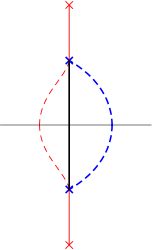
(a) Cut contours

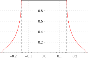
(b) Absolute densities along the condensate and the tails

Figure 37: An example solution on line $\mathrm{C}_{0}$. The condensate and the tails lie on the imaginary line. The standard contours are shown as dashed lines. The filling fractions are $\alpha_{1}=-0.14$ (red/thin, $n_{1}=0$, $x_{\pm}=\pm 0.2726i$) and $\alpha_{2}=1/2$ (blue/thick, $n_{2}=1$, $x_{\pm}=0.146434i$). Cut one is completely hidden in the condensate.

As mentioned, a consequence of the fact that the phase space of consecutive mode numbers is connected is that the mode numbers can change by a continuous variation of the fillings. In particular, if one follows a straight horizontal line in Fig. 34 from the left to the right, the branch points cycle around each other while the mode numbers decrease until the configuration reaches line $\mathrm{C}_{0}$ and both pairs of branch points and the contour lie on the imaginary line. A schematic sketch of this process is shown in Fig. 38.

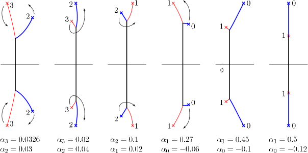
Figure 38: A sequence of configurations that evolves through the global moduli space of consecutive mode numbers. During the sequence, the branch cuts cycle around each other. The mode numbers are indicated next to each branch point. Each time a branch point passes a contour, its mode number decreases by two. The total filling fraction $\alpha$ increases during the sequence; the individual filling fractions are indicated below each subfigure. The sequence roughly follows a straight horizontal line in Fig. 35 at $\tilde{E}/4\pi^{2}\approx 0.3$. The final configuration lies on line $\mathrm{C}_{0}$, i.e. all branch points lie on the imaginary line. The size of the cuts increases from left to right, the rightmost configuration is about 15 times larger than the leftmost.

The sequence can even be continued further by following it in reverse, but in the other (left) half of the complex plane: The mode numbers become negative, but all other physical quantities are the same as in the mirror solution with positive mode numbers. This means that there exist two copies of the space in Fig. 34, one for positive and one for negative mode numbers, and the two parts are connected through line $\mathrm{C}_{0}$.

Also the lines $\mathrm{B}_{n}^{\prime}$, $n>0$ of unstable one-cut solutions (as shown in Fig. 8c) can be followed until the branch points reach the imaginary axis, similar to the sequence of two-cut solutions that approaches line $\mathrm{C}_{0}$. At this point, also the fluctuation points $n_{*}=(n-1)$ and $n_{*}=(n-1)^{\prime}$ lie on the imaginary line and the filling of the branch cut reaches $\alpha=1/2$, as follows from (3.5). But, according to (3.3), this implies that $P=\pi n>\pi$. Since the maximal physical momentum on a lattice is $P=\pi$, the physical momentum is $P-2\pi$ for $P>\pi$. The maximal physical momentum $P=\pi$ is reached by the configurations on line $\mathrm{B}_{n}^{\prime}$ long before the branch points arrive at the imaginary axis. Reaching the regime of such high momenta is prevented by the phase transition discussed at the end of Sec. 5.4, which makes the one-cut solution transform into a two-cut solution at the critical value of the filling $\alpha_{\mathrm{crit}}=\alpha_{\mathrm{Y}_{n}}$. Physically, nothing peculiar would happen when the momentum would increase to values larger than $\pi$, but it is interesting to see that the two-cut solutions by themselves implement the restriction to momenta $|P|\leq\pi$, as can be seen in the pictures of the phase space in Fig. 34,35.

5.6 Stability and Gauge Theory States

The expositions of this section show that the moduli space of two-cut solutions has a very rich structure, even though only solutions with consecutive mode numbers have been considered. Most remarkably, there seem to be no unstable two-cut solutions: For all spectral curves with consecutive mode numbers there is a configuration of standard and condensate cuts that generate the curve and that do not violate the stability condition. Here, by stability condition is meant that the absolute density never exceeds unity at any point on the cut contour whose tangent is vertical:

$$|\rho(x_{0})|\leq 1\quad\text{for }\rho(x_{0})\sim i$$ (5.4)

Such critical point are always hidden in a condensate cut. Thus it may be conjectured that all classically admissible two-cut solutions are solutions of the Bethe equations in the thermodynamic limit. In fact, numerical tests show strong evidence in favour of this conjecture: For most of the cases discussed in the previous section, numerically exact Bethe root distributions that approximate the cut contours have been obtained, see Sec. 7.

A remark about suitable gauge theory states is appropriate at this point. Only spin chain states with a momentum $P\in 2\pi\mathbb{Z}$ correspond to gauge theory states. None of the solutions studied in this chapter satisfies this condition: All two-cut configurations with consecutive mode numbers have a non-zero momentum $0<P\leq\pi$. Nevertheless, all qualitative results should generalise to valid gauge theory states. Namely, configurations whose cut structure is point symmetric about the origin manifestly have a vanishing momentum $P$. It is reasonable to expect that such point symmetric solutions with mode numbers $(n,n+1)$ and $(-n,-n-1)$ and with symmetric fillings exhibit the same qualitative features as the solutions investigated here (such as condensate formation and connectedness of the moduli space). Some point-symmetric configurations of two-cut and degenerate multi-cut solutions are studied in the next section.

6 Moduli Space of Non-Consecutive Mode Numbers

All qualitative features of the general moduli space with arbitrary mode numbers can already be seen in the case of consecutive mode numbers, which was studied in the previous section. In general, cuts with non-consecutive mode numbers lie further away from each other and hence influence each other less. Some examples will be studied in this section.

6.1 Mode Numbers $n_{1}=1$, $n_{2}=3$

First, the comparatively simple space of solutions with mode numbers $n_{1}=1$ (cut one), $n_{2}=3$ (cut two) shall be exposed. It is shown in the $(\alpha,P/2\pi\alpha)$ plane in Fig. 39.

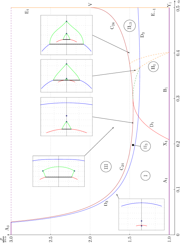
Figure 39: The space of solutions with mode numbers $n_{1}=1$, $n_{2}=3$, shown in the $(\alpha,P/2\pi\alpha)$ plane. Some example solutions in different regions are shown.

In region $\mathrm{I}$, the fillings of both cuts are small, their contours are disjoint and their absolute densities are bound by unity, hence there are no condensates. Line $\mathrm{D_{1}}$ marks the configurations in which the density on cut one equals $-i$. Beyond this line lies region $\mathrm{II_{1}}$, whose configurations have a condensate on cut one and an associated closed loop-cut with mode number $0=2^{\prime}$. Similarly, configurations on line $\mathrm{D_{2}}$ have an absolute density of $-i$ at the centre of cut two; beyond this line lies region $\mathrm{II_{3}}$, where cut two has a condensate core and an associated closed loop-cut with mode number $2=4^{\prime}$. In region $\mathrm{II_{13}}$, both cuts have a condensate core and associated closed loop-cuts. Finally, line $\mathrm{C_{24}}$ marks configurations in which the excitation points with mode numbers $n=2$ and $n=4$ have collided. Configurations beyond this line are unstable in the sense that they are degenerate cases of solutions with higher genus (higher number of cuts).

Regions $\mathrm{II_{1}}$ and $\mathrm{II_{13}}$ can be further subdivided, which is signified by the dashed and dotted lines in Fig. 39. To the left of these lines (at low total filling $\alpha$), the two cuts with their condensates and loop-cuts are disjoint. On the green, dashed line, the excitation point with mode number $2^{\prime}=4$ (which is the cusp of the loop-cut of cut two) collides with the condensate core of cut one. Upon further increasing the total filling, the condensate core of cut two (or its standard contour) collides with the condensate core of cut one; this event is marked by the orange, dotted line. At even higher total filling, the branch points of cut two pass through the condensate core of cut one (orange, dashed line), such that the whole contour of cut two (with its associated loop-cut) is encircled by the loop-cut of cut one. Nothing special happens to the condensate core of cut one during the passage of cut two – this is sensible, as the condensate core is invisible in the spectral curve $\mathrm{d}p$, which contains all the information about the solution. When cut two has completely passed through the condensate core of cut one, its mode number has changed to $n_{2}^{\prime}=n_{2}-2=1$.

When the total filling gets increased up to $\alpha=1/2$ (line $\mathrm{E_{-1}}$), the excitation point with mode number $2=0^{\prime}$, which marks the cusp of the closed loop-cut that is connected to cut one, reaches $x=\infty$. This results in a configuration similar to the one at the point $\mathrm{Y_{1}}$ (see Fig. 36): The contour of the closed cut passes through the branch points of cut one, such that cut one is completely hidden in a condensate that has two vertical, infinitely long tails. Consequently, the mode number of cut one is ambiguous: It is either $n_{1}=1$ or $n_{1}=-1$. In addition, there is cut two, whose mode number is $n_{2}^{\prime}=1$. It has a standard contour (below line $\mathrm{D_{3}}$), or a standard contour with a condensate core and a closed loop-cut (above line $\mathrm{D_{3}}$). At the upper end of line $\mathrm{E_{-1}}$ lies point $\mathrm{V}$, at which also the excitation point that marks the cusp of cut two’s closed loop-cut has reached $x=\infty$ and the configuration is completely symmetric about the origin (Fig. 40a).

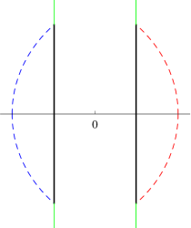
(a)

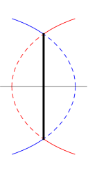
(b)

Figure 40: Configuration at point $\mathrm{V}$ in Fig. 39. This solution is symmetric about the origin and hence represents a valid gauge-theory state (The momentum equals $P=2\pi$). Figure LABEL:sub@fig:point_V_1 shows the configuration that is reached when coming from region $\mathrm{II_{13}}$ or from line $\mathrm{E_{-1}}$ in Fig. 39. There is a dual configuration of cuts, shown in LABEL:sub@fig:point_V_2, that generates the same solution. It has a “double-condensate” with root density $|\rho|=2$ at it’s centre.

$\longleftrightarrow$

Consequently, the momentum vanishes at this point, $P=2\pi$, and the solution represents a valid gauge-theory state. Fig. 40b shows another cut configuration that realises the solution at point $\mathrm{V}$. It can be constructed by taking another possible standard contour for each cut and replacing their common centre with a double condensate, that is a condensate with root density $|\rho|=2$. Bethe root distributions that show this type of pattern have been found before [10, 9]. Behind point $\mathrm{V}$ lies line $\mathrm{E_{1}}$. Configurations on this line are “mirror solutions” of the ones on line $\mathrm{E_{-1}}$: Cut three has mode number $1/-1$ and consists of a condensate with two vertical tails that extend to infinity, while cut one has mode number $-1$ and consists of a standard contour with or without a condensate core and an associated closed loop-cut.

6.2 Mode Numbers $n_{1}=1$, $n_{2}=-1$

The moduli space of solutions with mode numbers $n_{1}=1$ (cut one), $n_{2}=-1$ (cut two) is shown in Fig. 41,42 in the $(\alpha,P/2\pi\alpha)$ and in the $(\alpha,E)$ plane.

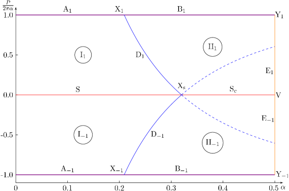
Figure 41: The space of configurations with mode numbers $n_{1}=1$, $n_{2}=-1$, shown in the $(\alpha,P/2\pi\alpha)$ plane. Configurations in regions $\mathrm{I}_{\pm 1}$ have plain standard contours, while configurations in regions $\mathrm{II}_{\pm 1}$ have condensates on either or both of the contours.

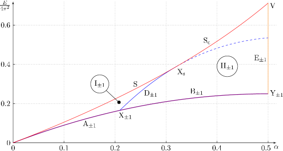
Figure 42: The space of configurations with mode numbers $n_{1}=1$, $n_{2}=-1$, shown in the $(\alpha,E)$ plane. Configurations that only differ by a reflection about the imaginary line have the same energy, hence the upper and the lower lines and regions of Fig. 41 lie on top of each other in this representation.

Regions, lines and points with the same labels but subscripts $1$ and $-1$ fall together in Fig. 42, since their configurations only differ by a reflection about the imaginary line and hence have the same energy.

As in previous examples, the lines $\mathrm{A}_{\pm 1}$ and $\mathrm{B}_{\pm 1}$ represent solutions with a single cut with mode number $n$, solutions on the lines $\mathrm{A}_{\pm 1}$ have a standard contour without a condensate core, while solutions on the lines $\mathrm{B}_{\pm 1}$ have a condensate core and a closed loop-cut. In the regions $\mathrm{I}_{\pm 1}$ and $\mathrm{II}_{\pm 1}$, both cuts with mode numbers $n_{1}=1$ and $n_{2}=-1$ are present. Line $\mathrm{D}_{\pm 1}$ separates solutions that only have a standard contour (region $\mathrm{I}_{\pm 1}$) from solutions that have a condensate core with a closed loop-cut (region $\mathrm{II}_{\pm 1}$). The closed loop-cut has mode number $n=0$ for both cuts. Hence on line $\mathrm{D}_{\pm 1}$, the absolute density at the centre of the cut with mode number $\pm 1$ equals $|\rho|=1$.

In the regions $\mathrm{I}_{1}$ and $\mathrm{II}_{1}$, the filling fraction of cut one is larger than the filling fraction of cut two, $\alpha_{1}>\alpha_{2}$. In the regions $\mathrm{I}_{-1}$ and $\mathrm{II}_{-1}$, it is the other way round, $\alpha_{1}<\alpha_{2}$. These regions are separated by the lines $\mathrm{S}$ and $\mathrm{S_{c}}$, which consist of symmetric solutions with $\alpha_{1}=\alpha_{2}$. Such solutions have vanishing momentum $P$ and hence represent valid gauge theory states, they were studied in [30]. Obviously, solutions on line $\mathrm{S}$ have plain standard contours, while solutions on line $\mathrm{S_{c}}$ have condensate cores in both contours. Point $\mathrm{X_{s}}$ marks the symmetric solution with maximal filling that does not have condensates. The lines $\mathrm{E}_{\pm 1}$ and point $\mathrm{V}$ are the same as the ones discussed above in Sec. 6.1, hence the diagrams in Fig. 39,41 are connected. The points $\mathrm{Y}_{\pm 1}$ actually both represent the same solution, namely the one shown in Fig. 36 whose cut configuration lies entirely on the imaginary line.

7 Numerical Solution of the Bethe Equation

In this section we develop a method for obtaining numerically exact distributions of Bethe roots for the Heisenberg spin chain. The main goal of this section is to test our predictions from the analysis of the one-cut and two-cut spectral curves in Sec. 3,5,6. Thus we are especially interested in distributions which can be compared with the spectral curve, i.e. solutions with large numbers of roots that align on a set of contours.

We examine in detail some subtle points of the previous analysis, such as stability (Sec. 2.7), condensate formation (Sec. 3.5) and phase transitions between spectral curves with different topologies (Sec. 5.4). We will see that condensate cores with roots separated by $\Delta u\approx i$ indeed appear in all cases considered. We will also confirm that the phase transition from one-cut to two-cut solutions indeed happens. Furthermore, in Sec. 7.3 we will analyse small deviations from the thermodynamic limit. In particular we will numerically analyse the leading finite-size corrections and show that they do not exhibit any non-analyticity due to the formation of the condensate.

The numerical configurations shown in this section are approximate solutions to the discrete Bethe equations (1.1) with finite length $L$. It is astonishing to observe how well the predictions from the thermodynamic limit describe the actual distributions of Bethe roots.

7.1 Description of the Numerical Method

Here we describe the numerical method used to solve the Bethe equations (1.1) in detail. In order to find roots of a set of equations numerically, it is important to specify a good set of starting points that are sufficiently close to the exact solution. We will focus on this problem first and then describe a simple programme for finding numerical solutions.

Starting Points.

In Sec. 2.3 we introduced the mode number associated to a branch cut in the thermodynamic limit. We will need to generalise the notion of mode numbers to the quantum case. The mode numbers naturally appear in the quantum theory when one takes the logarithm of (1.1):

$$iL\log\frac{u_{k}+\frac{i}{2}}{u_{k}-\frac{i}{2}}+2\pi n_{k}=\sum_{j\neq k}^{M}i\log\frac{u_{k}-u_{j}+i}{u_{k}-u_{j}-i}\,,\qquad k=1,\dots,M.$$ (7.1)

The integers $n_{k}$ represent the $2\pi i$-ambiguity of the logarithm, in the thermodynamic limit they exactly become the mode numbers introduced in equation (2.11). This can be seen by taking the large-$L$ limit of (7.1), as in [8, 9, 21]. The solution to (7.1) is uniquely specified by a set of integers $n_{k}$ (at least for large $L$ and small $M$).

In order to find the solution numerically by Newton’s method, one has to specify starting points for the search. For generic parameters it is very difficult to give suitable starting points that lead to convergent iterations. However, as we will see it is pretty simple to find good starting points in the limit of small filling fractions $L\gg M$ where the Bethe equations (7.1) can be solved approximately [10]:

To the leading order we can drop the r.h.s. of (7.1) and, assuming that $u_{k}\sim L$ (which is true in the case we are interested in), we get that $u_{k}\simeq L/2\pi n_{k}$. We conclude that Bethe roots with the same mode number $n_{k}$ are close to each other and separated by $\Delta u\sim L$ from other groups of roots with different mode numbers.

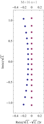
(a) $L=400$

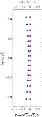
(b) $L=1600$

Figure 43: Approximation of a solution to the Bethe equations (1.1) by zeros of the Hermite polynomial for $M=16$ roots with mode number $n=1$ and chain lengths $L=400$, $L=1600$. Squares represent points given by $u_{k}=L/(2\pi n)+iz_{k}\sqrt{2L}/(2\pi n)$, where $z_{k}$ are zeros of Hermite polynomial of degree $M$, while circular dots represent numerically exact Bethe roots. This approximation provides us with a good set of starting points.

For resolving the positions of the Bethe roots with the same mode number $n$, we can neglect terms in the r.h.s. of (7.1) containing roots with different mode numbers and use the ansatz

$$u_{k}=\frac{1}{2\pi n}\left(L+iz_{k}\sqrt{2L}+\mathcal{O}(1/L^{0})\right).$$ (7.2)

Assuming that $n\sim 1$ and $z_{k}\sim 1$, we expand (7.1) and get [10]

$$\frac{1}{z_{k}-z_{j}}-z_{k}=0\,,$$ (7.3)

which is the equation for the zeros of the Hermite polynomial, $\mathrm{H}_{M}(z_{k})=0$. Numerically exact values of Bethe roots are plotted against their large-$L$ approximation (7.2) in Fig. 43, and one clearly sees that the relative mismatch is indeed smaller for larger $L$. It is possible to continue the $1/\sqrt{L}$ expansion in a systematic way to get a better description of Bethe roots for large $L$ and mode number $n$ fixed. For our goal the leading approximation of the Bethe roots by zeros of Hermite polynomials provides us with a good set of starting points for sufficiently large $L$.

Iteration Procedure.

Having starting points at hand it is almost immediate to construct a numerical solution of the Bethe equations using Newton’s method. However, we know the starting points only for large $L$. To overcome this difficulty we can view the Bethe root distributions as functions of the length $L$ while keeping the magnon number $M$ fixed. We can solve the Bethe equations numerically, gradually varying $L$ from a sufficiently large value $L\gg M$ to the desired value with $L=\mathcal{O}(M)$. In each step we use the numerical solution obtained in the previous step as new starting values for smaller $L$. In this way we obtain a series of configurations whose filling $\alpha=M/L$ slowly increases. Some important examples of such series will be considered in the next subsection.

For various reasons it is favourable to use the Bethe equations in product form (1.1) and not in logarithmic form (7.1) for the Newton iteration. Using this method, the mode numbers enter into the calculation only through the starting points. Since we vary $L$ slowly, at each step we inherit the information about the mode numbers from the previous step, and hence the resulting configuration corresponds to the analytically continued curve from the regime of large $L$.

Note that for large $L$ and fixed $M$ the roots are separated by $\Delta u\sim\sqrt{L}$ and thus the stability condition is satisfied, $|\rho|\approx 1/\Delta u\ll 1$. However, when we decrease $L$, at some point the separation between Bethe roots approaches $\Delta u=i$. The Bethe equations (1.1) are singular at this point which leads to a numerical instability at small $L$. Therefore the step size for $L$ must be chosen sufficiently small in this regime. For practical purposes one can even choose $L$ to take real intermediate values. We expect the above numerical procedure to lead to a reasonably unambiguous final configuration if $L$ is changed in sufficiently small steps.

Sample Programme.

Let us give a basic realisation of above method in Mathematica. For simplicity the programme presented in Tab. 2 is restricted to the one-cut case. To generalise it, it is enough to change the set of starting points u0 according to the discussion in the previous section. We tested this programme on Mathematica versions 5.2 and 6.0, but it should be compatible with earlier versions as well.

(*define mode number, number of roots, initial length and finial length*)
n = 1; M = 12; L = 100; Lfinal = 30;

(*starting points*)
u0 = (L/(2 Pi) + I Sqrt[2 L]/(2 Pi n) zk /. NSolve[HermiteH[M, zk] == 0, zk])

(*solve the Bethe equations while slowly decreasing the length L*)
Do[u0 = Table[u[k], {k, M}] /. FindRoot[Table[((u[k] + I/2)/(u[k] - I/2))^L ==
-Product[(u[k] - u[j] + I)/(u[k] - u[j] - I), {j, M}], {k, M}],
Table[{u[k], u0[[k]]}, {k, M}], WorkingPrecision -> 50, AccuracyGoal -> 20];
L-- // Print;
, {L - Lfinal + 1}]

(*plot the result*)
ListPlot[Transpose[{u0//Re,u0//Im}], PlotRange -> All, AspectRatio -> Automatic]

Table 2: Mathematica programme for the generation of a finite-length numerical Bethe root distribution corresponding to a one-cut spectral curve.

This programme can be optimised to work much faster, especially for the case of a large number of Bethe roots: A major improvement can be achieved by replacing the built-in FindRoot function, which is too general and inefficient, by a simple implementation of Newton’s method. Furthermore the step size for $L$ can be made adaptive. One can even decrease $L$ in small steps during each Newton iteration and thus avoid an excessively precise calculation which is merely used for new starting values.

7.2 Some Series of Numerical Solutions

In this section we will exploit numerical solutions of the Bethe equations obtained with our programme to test the predictions from the thermodynamic limit. We begin with a study of the simplest one-cut solution, subsequently proceed to more complex configurations with two cuts and consecutive mode numbers, and finish with a two-cut solution with non-consecutive mode numbers. In the last configuration, one of the two cuts transforms into a two-cut complex in a phase transition, the result being a three-cut solution.

One-Cut Solution, $n=1$.

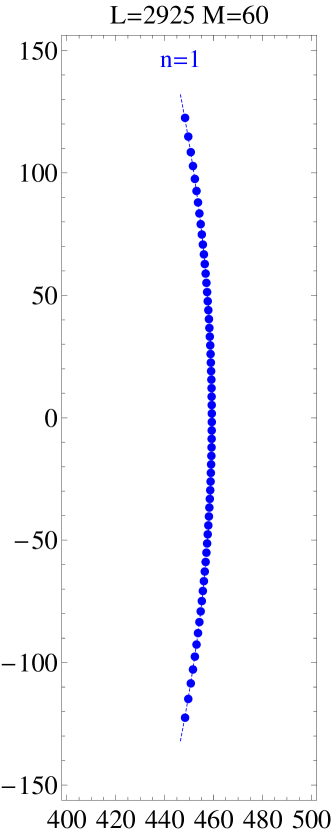
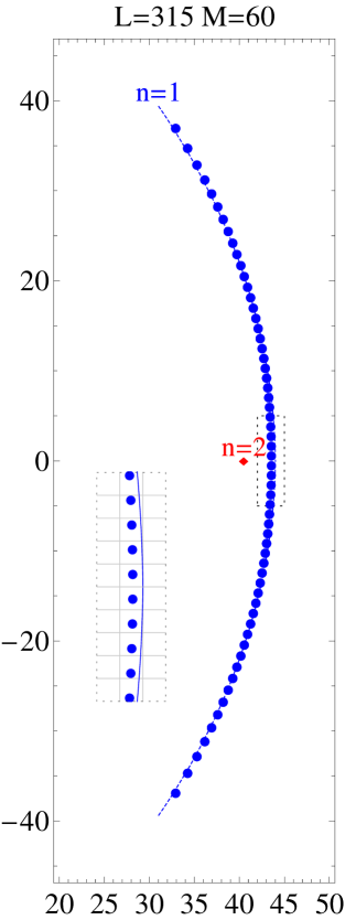
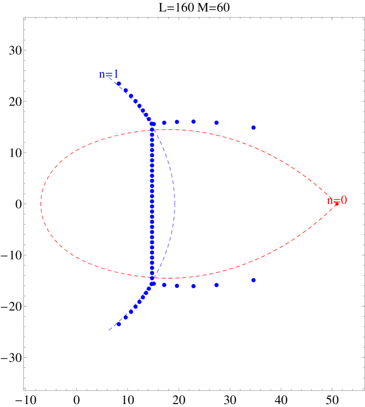
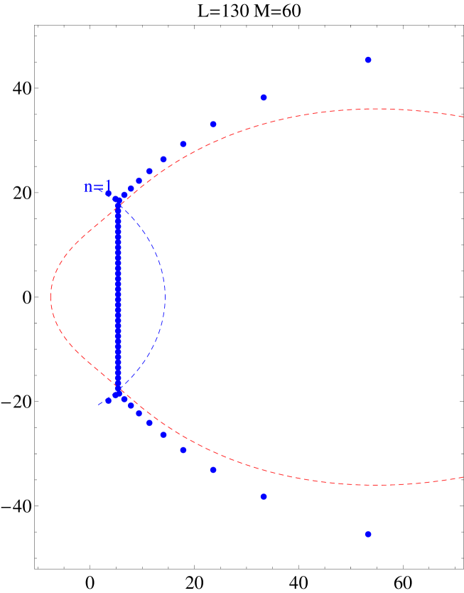
Figure 44: One-cut solutions with mode number $n=1$ and lengths $L=2925,315,160,130$. Shown are the cut contours of the spectral curve together with numerical solutions. When the maximum density along the cut exceeds $|\rho|=i$, the fluctuation point with mode number $n=2$ touches the cut. When we continue decreasing $L$, a condensate develops in the middle of the original cut and two extra tails appear. In fact in the scaling limit $L\sim M$ the two tails to the right are touching at the point of the virtual excitation, cf. Sec. 3.5.

In the thermodynamic limit this solution is discussed in Sec. 3. An interesting phenomenon which we expect to arise for this configuration is the appearance of a closed loop-cut for filling fractions above $\alpha_{\mathrm{cond}}$ (see Fig. 8b).

The spectral curve of the one-cut solution can be discussed very explicitly, in particular the quasi-momentum is given by a simple algebraic formula (3.1) and one can find the shape of the physical branch cut quite easily. In the first figure of Fig. 44 the contour is shown together with the numerical solution for $M=60$ roots and length $L=2925$. We almost do not see any deviation of the roots from the asymptotical curve. On the next picture we considerably increased the filling fraction to $M/L=60/315\approx 0.19$, and one can see that the distance between roots close to the real axis is just slightly above $i$. This means that the filling $\alpha$ is very close to $\alpha_{\mathrm{cond}}$ and the stability condition is almost violated. According to the discussion in Sec. 3.5, this implies that the fluctuation with mode number $2$ is very close to the cut. In the figure, we indicate it by a red diamond.

When we continue increasing the filling fraction to values above $\alpha_{\mathrm{cond}}$, the fluctuation point passes through the cut contour and produces a loop cut. At the intersection point of the loop cut with the original standard cut we expect the condensate to be formed. As is demonstrated in Fig. 44, this is indeed the case.

We can almost reach the maximal filling $\alpha={\textstyle\frac{1}{2}}$ numerically. As discussed in Sec. 5.5, this would correspond to a configuration with a condensate centred at the origin together with two tails that extend along the imaginary axis towards the fluctuation point, which has diverged to infinity.

Finally, we notice that the roots belonging to the two tails on the right of the condensate do not seem to align on the contour predicted by the spectral curve (red/dashed). In fact this is an artefact of the finiteness of the number of roots. One can observe that the situation becomes better when the number of roots $M$ is increased (while the filling fraction $M/L$ is held fixed). The finite-size effects become very relevant at the tip of the loop because the density drops to zero at the fluctuation point forming the tip. Close to a standard branch point the roots align on the contour more accurately, because the density decreases only as the square root of the distance from the branch point, whereas at the cusp of the loop the density is proportional to the distance itself and hence the deviation from the spectral curve is more severe.

One-Cut Solution, $n=2$.

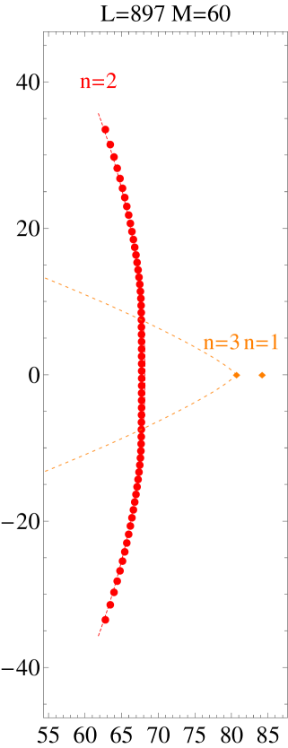
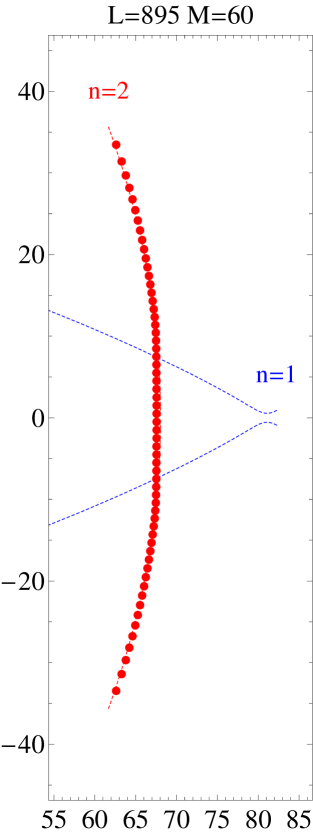
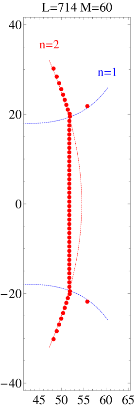
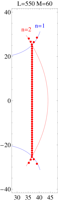
Figure 45: The one-cut configuration with mode number $n=2$ transforms into a two-cut configuration after the collision of the two fluctuation points with mode numbers $n=1,3$.

For larger mode numbers, the one-cut solution behaves similarly to the $n=1$ case when the filling fraction is increased. However, we expect that a configuration with $n>1$ exhibits a new type of behaviour when its filling fraction reaches $\alpha_{\mathrm{crit}}$ given by (3.15). As discussed in Sec. 3.5, we expect that a phase transition from one cut to two cuts occurs.

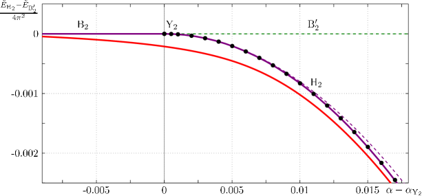
Figure 46: Shown is the same diagram as in Fig. 33. In addition, the energies of a series of numerical solutions to the discrete Bethe equations that start as a one-cut solution with mode number $n=2$ (red/solid) are displayed. The graph shows that the one-cut solution (line $\mathrm{B_{2}}$) indeed transforms into a two-cut solution (line $\mathrm{H_{2}}$) when the two fluctuation points collide (point $\mathrm{Y_{2}}$). The deviation from the exact thermodynamic lines is due to the finite length and number of roots in the numerical solutions.

In Fig. 45, we compare the distributions of numerical Bethe roots with mode number $n=2$ for different filling fractions. We see that the condensate forms when the nearest fluctuation from the left crosses the cut contour at $\alpha=\alpha_{\mathrm{cond}}$, which is in full agreement with the prediction of Tab. 1. In contrast to the $n=1$ case, there is also a fluctuation point to the right of the cut (with mode number $n=1$), even at small fillings $\alpha$. When we increase $\alpha$, the fluctuation point with mode number $n=3$, which initially was on the left of the standard cut, passes through the cut and approaches the fluctuation point with mode number $n=1$ (second figure in Fig. 45). Beyond the point of collision there are two possibilities – the configuration could continue as a one-cut solution (with a loop cut with two cusps that could naturally be decomposed into two standard cuts), or it could transform into a two-cut solution with lower energy as explained in Sec. 3.5. We found that in our study always the second possibility is realised, our numerical method prefers the two-cut configuration with lower energy. It seems that this configuration is numerically more stable. In particular we see that in the last two pictures of Fig. 45 the roots perfectly follow the two standard contours of the two-cut spectral curve. Accordingly, Fig. 46 shows that the energy of the numerical configuration after the point of collision matches the energy of the two-cut configuration (up to deviations due to finite-size effects), which clearly indicates that the phase transition is indeed taking place.

Two-Cut Solution, $n=1,2$.

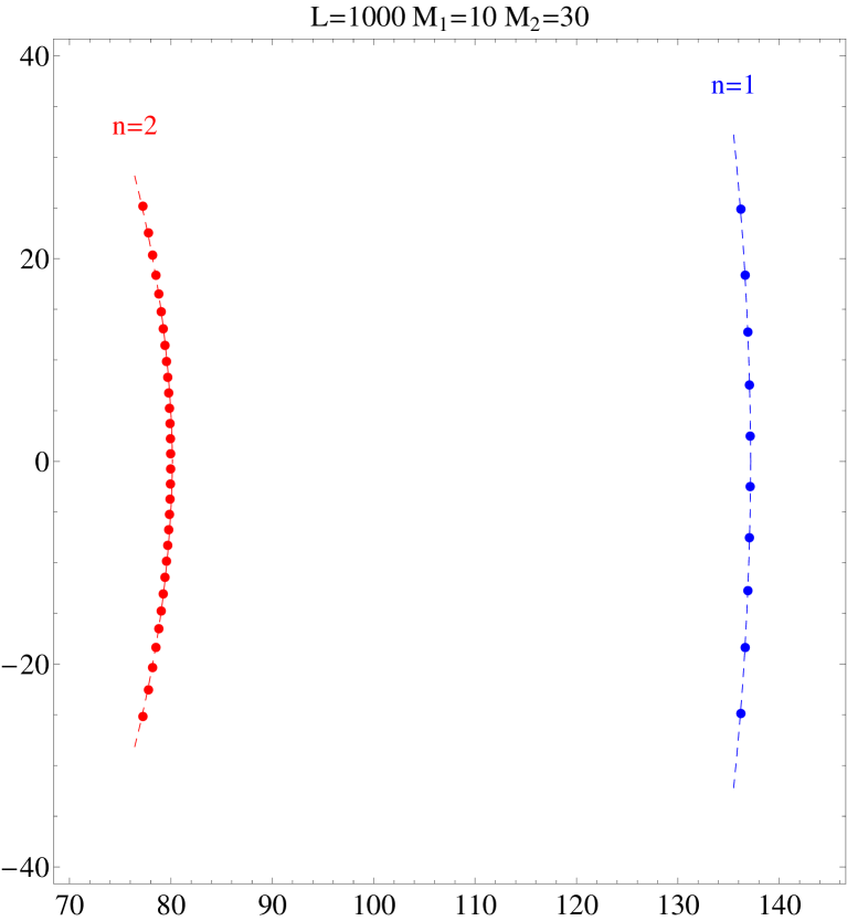
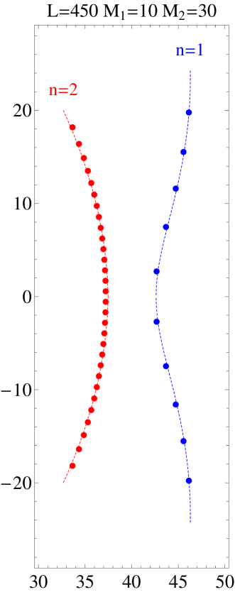
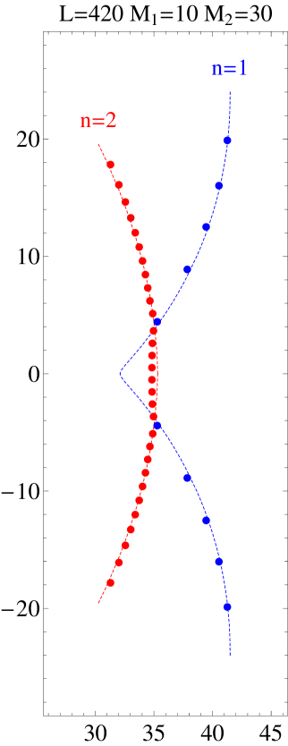
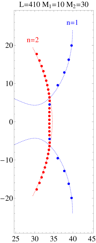
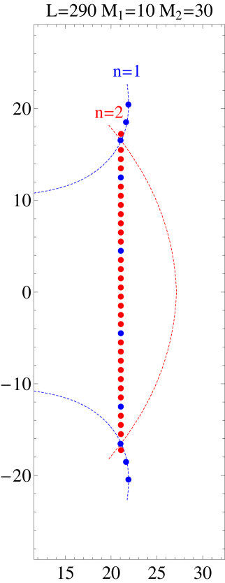
Figure 47: Two-cut solutions with consecutive mode numbers $n=1$ (right, blue) and $n=2$ (left, red) for different values of the length $L$. The intersection points of the two standard contours are connected by a vertical condensate cut.

The spectral curve for two-cut solutions was constructed in Sec. 4 and is less simple than the one-cut curve. The moduli space of two-cut configurations is also much more complicated, for the case of consecutive mode numbers it is described in detail in Sec. 5. Numerically, however, it is not difficult to construct a solution with an arbitrary number of cuts. We mainly want to show here that, in accordance with the prediction of Sec. 5, an intersection of the two cuts leads to the formation of a condensate that connects the two intersection points.

In Fig. 47 we compare numerical two-cut solutions with mode numbers $n=1,2$ with the predictions from the spectral curve. In the first two pictures the two cuts are disjoint and hence we are in region $\mathrm{I}_{12}$ of the phase diagram shown in Fig. 11. The last three configurations belong to region $\mathrm{II}_{12}$, and we see that indeed a condensate with roots separated by approximately $i$ connects the intersection points of the two contours.

On the third picture, the right (blue) $n=1$ cut does not encircle the origin of the complex plane, but it has a cusp at the point of intersection with the real axis. This means that this configuration lies exactly on the line $\mathrm{G}_{12}$. In the last configuration shown in Fig. 47, the branch points of the $n=2$ cut (red) are almost touching the $n=1$ cut (blue) which means that the configuration is very close to the line $\mathrm{C}_{1}$.

Two-Cut Solution, $n=1,3$.

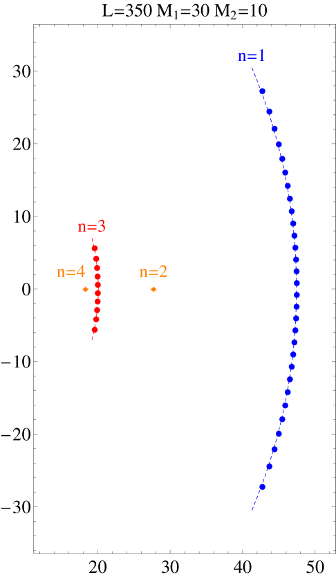
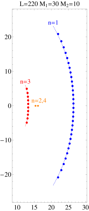
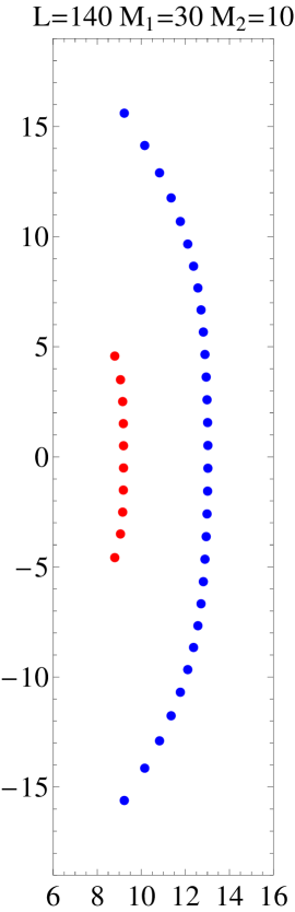
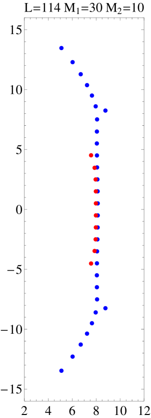
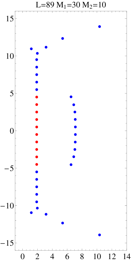
Figure 48: Two-cut solutions with non-consecutive mode numbers $n=1$ (blue) and $n=3$ (red) for different values of the length $L$. Both cuts develop condensates before they intersect each other. We see that the passage of one cut through the condensate core of the other does not affect the relative positions of the roots inside each cut.

Two-cut solutions with non-consecutive mode numbers allow for even richer properties. As is explained in Sec. 6.1, for some values of filling fractions both cuts can develop condensate cores before intersecting with each other. At higher fillings the cut with the higher mode number, which initially lies further left, can pass through the condensate core of the other cut. As explained in Sec. 6.1, this should not affect the inner structure of the cuts.

From the distributions of numerical roots for different values of the fillings in Fig. 48, we see indeed that the group of $n=3$ Bethe roots (left, red) reaches the condensate core of the $n=1$ roots (right, blue) and passes through the condensate. These numerical solutions confirm that the passage of a cut complex through a condensate core does not affect the structure of the individual complexes, i.e. their shape and their root densities.

We did not plot cut contours for all configurations in this case, because similarly as in the previous example, the configuration undergoes a phase transition. Namely, this series of configurations follows the line $P/2\pi\alpha=1.5$, which is slightly above the critical value $\sim 1.4$ so that we are crossing the line $\mathrm{C}_{24}$ of the Fig. 39. When the two fluctuations denoted by the orange diamonds ($n=2,4$) collide, the corresponding spectral curve transforms into a three-cut curve, as is expected from the discussion in Sec. 6.1. Note that we have no means to plot the exact contours for three-cut configurations and thus these lines are missing from the figures.

Conclusions.

We have presented numerical solutions for various types of configurations discussed in this paper, and in all cases we observe a perfect match with the analytical predictions of the spectral curve. This confirms the validity of the analysis of the thermodynamic limit in the previous sections.

7.3 One-Cut Solution and Finite-Size Effects

In this paper we mainly focus on the strict thermodynamic limit. However, the numerical solutions containing a finite number of Bethe roots allow us to easily analyse the leading correction to the thermodynamic limit. In string theory they correspond to the semiclassical energy shift, see [33, 34, 35] for a general discussion of canonical quantisation for the spectral curve.

The energy shift was studied analytically for one-cut configurations of the Heisenberg spin chain in [23, 26, 25]. The result reads

$$E^{(1)}=4\pi^{2}\left[\sum_{k=1}^{\infty}\left(k^{2}\sqrt{1-\frac{4n^{2}\alpha(1-\alpha)}{k^{2}}}-k^{2}-2n^{2}\alpha(1-\alpha)\right)-n^{2}\alpha(1-\alpha)\right].$$ (7.4)

Note that this result equals the sum of zero-mode energies of the fluctuation modes in (3.13) upon zeta-function regularisation of the sum. The result may in principle include exponentially suppressed contributions, see [36, 37]. It is however conceivable as well that these corrections are absent in the Heisenberg/Landau–Lifshitz spectral curve which is considerably simpler than the spectral curve for the principle chiral model/string theory.

The above energy shift was obtained assuming that the roots are distributed along a single cut and it is a priori questionable if this result remains true for the case $\alpha>\alpha_{\mathrm{cond}}$ when the loop cut appears and the distribution of roots is more sophisticated. We can however use the intuition gained studying the strict thermodynamic limit: We saw that the energy is described by the same analytical expression (3.3) before and after the condensate is formed. Therefore we expect (7.4) to be valid also in the full range of $\alpha$’s.

Here we perform a numerical test of this natural guess. In Tab. 3 we give a series of deviations of numerical values of the energy from their asymptotical values (3.3) for different numbers of roots and for two fixed filling fractions below and above the point of condensation $\alpha_{\mathrm{cond}}\approx 0.21$. To compute $\delta E_{\infty}$ we fit the values of the energies from the table for finite $M$ by a constant and inverse powers of $M$. The value of the constant is precisely $\delta E_{\infty}$ given in the table. For both filling fractions we see a perfect match with the value given by (7.4), which shows that the correction (7.4) is also valid for fillings beyond $\alpha_{\mathrm{cond}}$.

$\begin{array}[]{|c||c|c|c|c|c|c|c||c|}\hline\cr\alpha&\delta E_{10}&\delta E_{20}&\delta E_{30}&\delta E_{40}&\delta E_{50}&\delta E_{60}&\delta E_{\infty}&E^{(1)}\\ \hline\cr 0.10&\phantom{+}2.372&\phantom{+}2.356&\phantom{+}2.351&\phantom{+}2.349&\phantom{+}2.347&\phantom{+}2.346&\phantom{+}2.3411&\phantom{+}2.3411\\ \hline\cr 0.33&-2.273&-2.472&-2.539&-2.573&-2.594&-2.608&-2.6768&-2.6769\\ \hline\cr\end{array}$

Table 3: Deviations $\delta E_{M}$ of the numerical energy from its asymptotical value for different numbers $M$ of Bethe roots and for two fixed filling fractions $\alpha$ above and below $\alpha_{\mathrm{cond}}\approx 0.21$. $\delta E_{\infty}$ is the extrapolation to an infinite number of roots. The value $E^{(1)}$ (7.4) is given for comparison.

A possible explanation for this could be based on the algebraic curve. The algebraic curve appearing in the thermodynamic limit can be modified to reproduce also the leading quantum corrections [25, 27]. The same type of analysis we have performed for the leading order hopefully can be applied for this corrected curve as well.

8 Conclusions and Outlook

In this article we have considered the general solution (Sec. 2) for the spectrum of the Heisenberg ferromagnet in the thermodynamic limit by means of spectral curves. Equivalently, we have studied the semiclassical Landau–Lifshitz model on $S^{2}$, see App. A. In particular, we have constructed the general two-cut (elliptic) solution (Sec. 4) and studied its properties (Sec. 5,6). This allowed us to shed light on the issue of quantum stability of classical solutions (Sec. 3,5) brought up in [23, 25]. We have also tested our claims by constructing some numerical solutions (Sec. 7). Let us summarise our findings briefly:

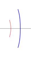
(a) $\alpha_{1,2}$ small

(b) $\alpha_{1,2}$ large

Figure 49: Typical configurations of the two main types of two-cut solutions. When the fillings $\alpha_{1,2}$ are small, the two cuts are disjoint LABEL:sub@fig:conctwocuta. When the fillings increase, the cuts attract each other and eventually collide, forming a condensate at their common centre LABEL:sub@fig:conctwocutb.

The two-cut solution is specified by two mode numbers $n_{1,2}$ and two fillings $\alpha_{1,2}$. Its quasi-momentum is an elliptic function which encodes all the relevant classical observables. In order to quantise this solution, one needs to understand the positions of the two branch cuts which correspond to the distribution of Bethe roots. We have studied these in detail and we have found a rich “phase space” (Fig. 34,39) of different configurations depending on the fillings.

There are two main configurations, see Fig. 49: When the fillings are sufficiently small, there will be two separate branch cuts, see Fig. 49a. When the fillings are increased, the branch cuts bend towards each other so that they eventually would overlap. Instead of overlapping, a straight vertical condensate of Bethe roots with constant density forms. The configuration looks like a Bethe string but with four curved tails of lower density, see Fig. 49b.

Classically there is no quantitative difference between the two types of solutions, but the condensate serves several purposes for the quantum model: It sets an upper bound to the density of Bethe roots which is an important feature for quantum stability. In some sense, the condensate “hides” some potentially dangerous distributions of Bethe roots on an unphysical sheet of the spectral curve. Moreover, solutions with different mode numbers (but equal $n_{1}-n_{2}$) can be connected analytically via the condensate. For example, there is only a single connected phase space for solutions with consecutive mode numbers ($n_{2}=n_{1}+1$). Finally, we have observed that the naturally continued overall momentum $P$ never crosses the boundary of the first Brillouin zone; it is apparently bounded by $|P|\leq\pi$ and the condensate formation plays an important role. At $P=\pm\pi$ the two-cut solution (with consecutive mode numbers) flattens out onto the imaginary axis where it connects smoothly the two regimes with $P>0$ and $P<0$.

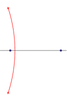
(a) $\alpha<\alpha_{\mathrm{cond}}$

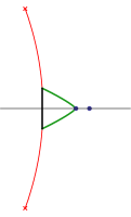
(b) $\alpha_{\mathrm{cond}}<\alpha<\alpha_{\mathrm{crit}}$

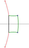
(c) $\alpha_{\mathrm{crit}}<\alpha$

Figure 50: The three qualitatively different types of one-cut solutions. For small fillings, the single cut is manifestly stable LABEL:sub@fig:conconebubblecutsa. At intermediate fillings, the cut obtains a condensate and an additional closed loop cut with a cusp; a potential instability is hidden in the condensate LABEL:sub@fig:conconebubblecutsb. When the filling becomes large, the classical solution acquires unstable fluctuation modes and the closed loop cut has two cusps LABEL:sub@fig:conconebubblecutsc. Nevertheless, the configuration is physical, albeit with non-minimal energy; see the discussion in the main text.

(a) $\alpha<\alpha_{\mathrm{cond}}$

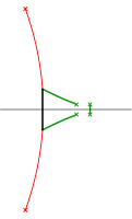
(b) $\alpha_{\mathrm{cond}}<\alpha<\alpha_{\mathrm{crit}}$

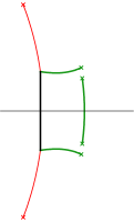
(c) $\alpha_{\mathrm{crit}}<\alpha$

Figure 51: The configurations in Fig. 50b,50c should be understood as degenerate cases of two- and three-cut solutions. This can be seen by the addition of small but macroscopic numbers of Bethe roots to the fluctuation points, which “regularises” the configurations. The resulting configurations in LABEL:sub@fig:conconebubblecutsregb, LABEL:sub@fig:conconebubblecutsregc are perfectly well-behaved two- and three-cut solutions. Exciting the fluctuation points of the solution in Fig. 50c lowers the energy, which is consistent with the (only seemingly) unstable excitation modes.

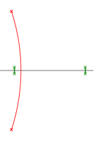
(a) $\alpha<\alpha_{\mathrm{cond}}$

(b) $\alpha_{\mathrm{cond}}<\alpha<\alpha_{\mathrm{crit}}$

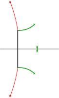
(c) $\alpha_{\mathrm{crit}}<\alpha$

Figure 52: The proper physical continuation of the one-cut solution beyond the critical filling $\alpha_{\mathrm{crit}}$ is the two-cut solution, Fig. 10e. Unlike the degenerate three-cut solution, Fig. 50c, this configuration locally minimises the energy. The phase transition from the one-cut to the two-cut solution occurs when the right fluctuation point collides with the cusp of the closed loop cut. Shown here is the regularised version of this process, where the fluctuation points carry a small but finite number of excitations.

Concerning quantum stability we find that an instability does not actually put a threat to the quantisation of some classical solution; the instability is rather caused by an unsuitable way of looking at the classical solution. This can be observed conveniently by means of the one-cut solution (Fig. 50) Here there are three main classes of cut configurations (which serve as subclasses for the two-cut solution):

For small filling, there is just a simple cut, see Fig. 50a, in which case the solution is perfectly stable. For intermediate filling the naive one-cut solution violates the stability criterion but without any observable flaws like unstable fluctuation modes. In this case, the physical cut configuration develops a condensate and a loop with a cusp, see Fig. 50b, which achieves to bypass the stability criterion; it is nevertheless semiclassically equivalent to the one-cut solution. For large filling, the naive one-cut solution acquires an unstable fluctuation mode which appears to render the solution unphysical. The physical cut configuration now has a condensate and a loop with two cusps, see Fig. 50c, which gives a clue of how to understand the instability:

The latter two dressed configurations should be interpreted as singular limits of two-cut or three-cut solutions, respectively, see Fig. 51. In the naive one-cut configuration, a fluctuation would break apart the loop at a cusp by a tiny amount. This is fine when the cusp is on the real axis (for intermediate filling), but away from the real axis (for large filling) it leads to complex momenta and thus an instability. Conversely, fluctuations of the regularised three-cut configuration would merely change the filling of either the two-cut complex or the third cut; in either case the configuration remains symmetrical with respect to the real axis, and there is no physical instability. Therefore the classical one-cut state with large filling does have a corresponding quantum state. This state however does not minimise the energy locally in accordance with the apparent instability. The energy is lowered by taking away Bethe roots from the third cut and moving them onto the two-cut complex. At the end of this process the third cut has evaporated and only the two-cut complex remains which is a genuine two-cut solution (Fig. 52c,10e).

This leads to the conclusion that the one-cut solution undergoes a phase transition at the point which separates intermediate and large filling: When the one-cut solution is analytically continued from small to large filling one obtains a degenerate three-cut solution. However in the vicinity of the latter there exists a two-cut solution with slightly smaller energy. It is useful to consider this solution the proper physical continuation of the one-cut curve. We find that at the phase transition point the second derivative of the energy is discontinuous. An exact expression for the discontinuity has been found on the basis of numerical data; an analytic confirmation of its form would be desirable. Technically, the phase transition turns out to be equivalent to the one observed in 2D QCD on $S^{2}$ [32] or equivalently a particular matrix model. In App. B we summarise the relevant functions and illustrate the phase transition for that model. Note that the apparent instability and the phase transition are merely artefacts of the thermodynamic limit in accordance with general results of statistical physics; they are resolved naturally at finite size, i.e. by the quantum theory: At finite $L$ there exists no precise notion of continuous cuts and the distribution of Bethe roots onto these cuts is often ambiguous. Thus two cuts never actually end on the very same point which was an essential assumption for the instability and the phase transition. In particular we show that numerically exact solutions with finite $L$ are smoothly interpolating between two phases and there is no real instability when the condensate forms.

We hope to have presented a fairly complete picture of the Heisenberg ferromagnet in the thermodynamic limit, its quantum fluctuations and the issue of stability. However there are several further questions which may be addressed in future work. One of them would be how precisely the third cut interacts with the two-cut complex in solutions of the type shown in Fig. 50c,51c. An investigation of this issue would require an explicit expression for the (hyperelliptic) three-cut quasi-momentum. Further, it would be interesting to construct the general elliptic solution to the Landau-Lifshitz model which includes the solutions obtained in [18, 38]. It should be equivalent to the two-cut solution presented here and the circular solution (A.8) should transform into the elliptic solution in the same way the two-cut solutions emerges from the one-cut solution at large fillings. Another question would be how the thermodynamic solutions of the Heisenberg magnet behave under the influence of a magnetic field and how this would change the picture of the phase space.

Concerning the AdS/CFT correspondence, a generalisation of the results to the $\mathrm{SU}(2)$ principal chiral model describing the dual string theory on $\mathbb{R}\times\mathrm{S}^{3}$ would be desirable. As discussed in [21], the solution to this model is given by a spectral curve that reduces to the Heisenberg spectral curve in a certain limit. Because of their strong structural similarity, we expect that stability and loop-formation work in qualitatively the same fashion. The phase space of general two-cut solutions (or elliptic string states) is likely to be similar as well, but new features may appear due to the more elaborate singularity structure on the curve. Therefore it is worth obtaining and discussing the general two-cut curve for the principal chiral model. Some special cases of two-cut solutions have appeared in [30, 39]. Analogously one could find the corresponding elliptic solution of the equations of motion explicitly, e.g. using the results of [33, 34]. This solution may be related to the solutions studied in [40, 41].

Finally, it remains an open question whether a similar study of the thermodynamic phase space can be carried out for spin chains which have different symmetry groups, quantum-deformed symmetry, or for which the spins transform in different representations. For example, studying the spectrum for symmetry groups of higher rank requires working with spectral curves with more than two sheets, which complicates the analysis substantially. Moreover for more general symmetry groups the algebraic curves are quite sensitive to different boundary conditions of the spin chain [27], thus making the analysis even more complicated (and interesting).

Acknowledgements

We would like to thank V. Bazhanov, V. Kazakov, M. Staudacher and P. Vieira for interesting discussions.

The work of N.G. was partially supported by a French Government PhD fellowship, by RSGSS-1124.2003.2 and by RFFI project grant 06-02-16786. N.G. was also partly supported by ANR grant INT-AdS/CFT (contract ANR36ADSCSTZ). N.G. thanks the AEI Potsdam, where part of this work was done, for the hospitality during the visit.

Appendix A The Landau–Lifshitz Model

The long-wavelength limit of the Heisenberg ferromagnet is equivalent to the Landau–Lifshitz model on $\mathrm{S}^{2}$ [19, 18], see also [42] for a review of Landau–Lifshitz models in connection with the AdS/CFT correspondence. Here we shall discuss the simplest circular solution and its fluctuation spectrum which corresponds to the one-cut solutions discussed in Sec. 3.

A.1 Definitions

The Landau–Lifshitz model on $S^{2}$ is a classical two-dimensional sigma model with two fields $\theta(\sigma,\tau)$ and $\phi(\sigma,\tau)$ which are the standard angular coordinates on $S^{2}$. We identify the site $k$ of the corresponding Heisenberg chain with the coordinate $\sigma=2\pi k/L$ of the sigma model. The expectation value of the spin projection $S_{z}$ at that site corresponds to the value ${\textstyle\frac{1}{2}}\cos\theta$ at $\sigma$.

In analogy to the closed spin chain we take the world sheet to be closed, i.e. the coordinate $\sigma$ is identified with $\sigma+2\pi$: Consequently, the embedding coordinates $\theta$ and $\phi$ (more precisely the equivalence classes describing points on $S^{2}$) must be $2\pi$-periodic in $\sigma$. This leads to the following periodicity conditions

$$\theta(\sigma+2\pi,\tau)\in\pm\theta(\sigma,\tau)+2\pi\mathbb{Z}\,,\qquad\phi(\sigma+2\pi,\tau)\in\phi(\sigma,\tau)+2\pi\mathbb{Z}+{\textstyle\frac{1}{2}}\pi(1\mp 1).$$ (A.1)

The Lagrangian reads

$$\mathcal{L}=-\frac{L}{4\pi}\,\dot{\phi}\cos\theta-\frac{\pi}{2L}\bigl{(}\theta^{\prime\,2}+\phi^{\prime\,2}\sin^{2}\theta\bigr{)},$$ (A.2)

where the constants $L/4\pi$ and $\pi/2L$ are adjusted to match with our conventions for the Heisenberg chain. In fact the first term in the Lagrangian originates from a topological Wess–Zumino term in three dimensions and for a fully consistent treatment one should make the replacement

$$\dot{\phi}\cos\theta\to\int_{0}^{1}\left(\frac{\mathrm{d}\phi}{\mathrm{d}\tau}\,\frac{\mathrm{d}\cos\theta}{\mathrm{d}r}-\frac{\mathrm{d}\phi}{\mathrm{d}r}\,\frac{\mathrm{d}\cos\theta}{\mathrm{d}\tau}\right)\mathrm{d}r.$$ (A.3)

The equations of motion following from the Lagrangian are

$$\dot{\theta} =\left(\frac{2\pi}{L}\right)^{2}\bigl{(}2\theta^{\prime}\phi^{\prime}\cos\theta+\phi^{\prime\prime}\sin\theta\bigr{)},$$

$$\dot{\phi} =\left(\frac{2\pi}{L}\right)^{2}\bigl{(}\phi^{\prime\,2}\cos\theta-\theta^{\prime\prime}\csc\theta\bigr{)}.$$ (A.4)

Taking the derivative of $\mathcal{L}$ with respect to $\dot{\theta}$ and $\dot{\phi}$ yields the conjugate momentum densities

$$\pi_{\theta}=0\,,\qquad\pi_{\phi}=-\frac{L}{4\pi}\cos\theta.$$ (A.5)

The Lagrangian is homogeneous and therefore the total energy and total momentum are conserved. The rescaled total energy and a suitably shifted total momentum read

$$\tilde{E}\mathrel{} = \mathrel{}EL=L\int\bigl{(}\pi_{\theta}\dot{\theta}+\pi_{\phi}\dot{\phi}-\mathcal{L}\bigr{)}\mathrm{d}\sigma=\frac{\pi}{2}\int\bigl{(}\theta^{\prime\,2}+\phi^{\prime\,2}\sin^{2}\theta\bigr{)}\mathrm{d}\sigma,$$

$$P\mathrel{} = \mathrel{}\frac{1}{2}\int\phi^{\prime}\,\mathrm{d}\sigma+\frac{2\pi}{L}\int\bigl{(}\pi_{\theta}\theta^{\prime}+\pi_{\phi}\phi^{\prime}\bigr{)}\,\mathrm{d}\sigma=\frac{1}{2}\int\bigl{(}1-\cos\theta\bigr{)}\phi^{\prime}\,\mathrm{d}\sigma.$$ (A.6)

Furthermore the Lagrangian is invariant under shifts $\phi\mapsto\phi+\varepsilon$ which yields the conserved total spin $S=L({\textstyle\frac{1}{2}}-\alpha)$ with the filling

$$\alpha=\frac{1}{2}+\frac{1}{L}\int\pi_{\phi}\,\mathrm{d}\sigma=\frac{1}{4\pi}\int\bigl{(}1-\cos\theta\bigr{)}\,\mathrm{d}\sigma.$$ (A.7)

A.2 Circular Solution

The simplest non-trivial solution of the Landau–Lifshitz model is the circular string at constant latitude $\theta_{0}$ with $n$ windings [21]

$$\theta(\sigma,\tau)=\theta_{0},\qquad\phi(\sigma,\tau)=n\sigma+(2\pi/L)^{2}n^{2}\tau\cos\theta_{0}.$$ (A.8)

It has the same charges as the one-cut solution of the Heisenberg magnet (3.3)

$$\alpha={\textstyle\frac{1}{2}}\bigl{(}1-\cos\theta_{0}\bigr{)},\qquad P=2\pi n\alpha,\qquad\tilde{E}=4\pi^{2}n^{2}\alpha(1-\alpha).$$ (A.9)

The momentum $P$ and the filling $\alpha$ are defined such that they both vanish for the vacuum solution at $\theta_{0}=0$

$$\alpha=P=\tilde{E}=0.$$ (A.10)

A.3 Fluctuations

We would like to obtain the spectrum of fluctuations around this solution. For the case of $\alpha={\textstyle\frac{1}{2}}$ this problem was solved in [43] which coincides with the ultra-relativistic limit of spinning strings discussed in [24]. To this end, fluctuation modes with Fourier mode $k$ and frequency $\omega_{k}$ are added to the background solution with the following ansatz

$$\delta\theta=\frac{a}{\sqrt{L}}\,\cos\bigl{(}k\sigma+\omega_{k}\tau+c\bigr{)},\qquad\delta\phi=\frac{b}{\sqrt{L}}\,\sin\bigl{(}k\sigma+\omega_{k}\tau+d\bigr{)}.$$ (A.11)

From the equations of motion it follows immediately that $d=c$ as well as

$$\omega_{k}=\left(\frac{2\pi}{L}\right)^{2}\left(2nk\cos\theta+\frac{b}{a}\,k^{2}\sin\theta\right)=\left(\frac{2\pi}{L}\right)^{2}\left(2nk\cos\theta+\frac{a}{b}\,\frac{k^{2}-n^{2}\sin^{2}\theta}{\sin\theta}\right).$$ (A.12)

This fixes the frequency and ratio of amplitudes

$$\omega_{k}\mathrel{} = \mathrel{}\left(\frac{2\pi}{L}\right)^{2}\left(2nk(1-2\alpha)+k^{2}\sqrt{1-\frac{4n^{2}\alpha(1-\alpha)}{k^{2}}}\right),$$

$$\frac{b}{a}\mathrel{} = \mathrel{}\frac{1}{2\sqrt{\alpha(1-\alpha)}}\sqrt{1-\frac{4n^{2}\alpha(1-\alpha)}{k^{2}}}\,.$$ (A.13)

Now it turns out that the total energy, total momentum and filling are not yet completely fixed. They still depend on the value of $a$ and curiously also on the second variation of the $\sigma$-independent mode

$$\delta^{2}\theta=\frac{f}{L}\,.$$ (A.14)

We shall parametrise our ignorance by two constants $N_{k}$ and $N_{0}$ as follows

$$a\mathrel{} = \mathrel{}\sqrt{2N_{k}}\bigg{/}\sqrt[\scriptstyle 4]{1-\frac{4n^{2}\alpha(1-\alpha)}{k^{2}}}\,,$$

$$b\mathrel{} = \mathrel{}\frac{\sqrt{N_{k}}}{\sqrt{2}\sqrt{\alpha(1-\alpha)}}\sqrt[\scriptstyle 4]{1-\frac{4n^{2}\alpha(1-\alpha)}{k^{2}}}\,,$$

$$f\mathrel{} = \mathrel{}\frac{1}{\sqrt{\alpha(1-\alpha)}}\left(N_{0}+N_{k}-N_{k}\frac{1-2\alpha}{2}\bigg{/}\sqrt{1-\frac{4n^{2}\alpha(1-\alpha)}{k^{2}}}\right).$$ (A.15)

This leads to the following shift in the observables

$$\delta^{2}\alpha\mathrel{} = \mathrel{}\frac{N_{0}+N_{k}}{L}\,,$$

$$\delta^{2}P\mathrel{} = \mathrel{}N_{0}\,\frac{2\pi n}{L}+N_{k}\,\frac{2\pi(n+k)}{L}\,,$$ (A.16)

$$\delta^{2}\tilde{E}\mathrel{} = \mathrel{}N_{0}\frac{4\pi^{2}n^{2}(1-2\alpha)}{L}+N_{k}\frac{4\pi^{2}}{L}\left(n(n+2k)(1-2\alpha)+k^{2}\sqrt{1-\frac{4n^{2}\alpha(1-\alpha)}{k^{2}}}\right).$$

The excitations enumerated by $N_{0}$ and $N_{k}$ carry each one quantum $1/L$ of filling equivalent to one unit of spin. They have mode numbers $n$ and $n+k$, respectively. Their energies can be read off from the above expression. It is not hard to see that a quantum of mode $n$ essentially just increases $\alpha$ by $1/L$ in the classical solution, cf. (A.9). The charges for mode $n+k$ are in complete agreement with the fluctuations in the ferromagnetic Heisenberg magnet (3.13). A careful semiclassical analysis actually shows that the numbers $N_{0}$ and $N_{k}$ must be integers.

The classical solution (A.8) is unstable if some of the oscillator frequencies $\omega_{k}$ are complex. Obviously, this is the case if

$$2n\sqrt{\alpha(1-\alpha)}>1\,.$$ (A.17)

The transition from stable to unstable classical solutions exactly happens at the critical density $\alpha_{\mathrm{crit}}$ (3.15), where the one-cut solution of the Heisenberg magnet transforms into a two-cut solution, as discussed in Sec. 5.4.

Appendix B The Douglas–Kazakov Transition

Here we shall review the Douglas–Kazakov transition [32] for QCD on $S^{2}$ on a technical level. It mimics the transition between our one-cut and two-cut solutions, albeit in a somewhat simplified and more transparent fashion.

B.1 Definitions

The description of the partition function in the large-$N$ limit of QCD on $S^{2}$ uses a density function $\rho(h)$ with support on the real axis. It must obey certain integral equations which will not be needed in detail here.

In order to extract the relevant observables it is convenient to introduce the continuation $u(h)$ of $\rho(h)$ into the complex plane. The function $u(h)$ has a branch cut on the real axis such that the real/principal part equals the density

$$\rho(h)={\textstyle\frac{1}{2}}u(h+i\epsilon)+{\textstyle\frac{1}{2}}u(h-i\epsilon).$$ (B.1)

The function $u(h)$ is the analog of our quasi-momentum $p(x)$ and its derivative $u^{\prime}(h)$ is an algebraic curve. Apart from the branch cut, the only singularity is at $h=\infty$ with

$$u(h)=\frac{1}{2\pi i}\left(-Ah+\frac{2}{h}+\frac{4}{h^{3}}\,(F^{\prime}+{\textstyle\frac{1}{24}})+\mathcal{O}(1/h^{5})\right)\,.$$ (B.2)

This expansion also defines the area $A$ and the derivative of the free energy $F^{\prime}$. It is clear that these quantities play similar roles as the total filling $\alpha$, momentum $P$ and energy $\tilde{E}$.

(a) rational regime, $A<A_{\mathrm{crit}}$

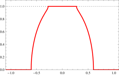
(b) elliptic regime, $A>A_{\mathrm{crit}}$

Figure 53: Density function $\rho(h)$ in the respective regimes.

B.2 Rational Regime

The simplest solution has one branch cut at $[-h_{\mathrm{max}},+h_{\mathrm{max}}]$. The function $u(h)$ consequently is of semi-circle form

$$u(h)=\frac{1}{2\pi}\sqrt{A(4-Ah^{2})}\,,$$ (B.3)

with $h_{\mathrm{max}}=2/\sqrt{A}$, see Fig. 53a.

The resulting free energy from (B.2) is simply [44]

$$F^{\prime}=\frac{1}{2A}-\frac{1}{24}\,.$$ (B.4)

This function is physically correct for $A\approx 0$. However, it was noticed that it does not have the correct behaviour at $A\to\infty$. For instance $F^{\prime}\to-\frac{1}{24}$ but not $F^{\prime}\to 0$.

B.3 Elliptic Regime

On the technical level, the pathology can be attributed to a density which grows beyond a threshold of

$$\rho_{\mathrm{max}}=1.$$ (B.5)

A density with $\rho(h)>1$ is unphysical. Indeed for $A>A_{\mathrm{crit}}$ with

$$A_{\mathrm{crit}}=\pi^{2}$$ (B.6)

the maximum density $\rho(0)=\sqrt{A}/\pi$ exceeds the maximum allowed density $\rho(0)>\rho_{\mathrm{max}}$.

This problem is resolved by inserting a condensate with constant density $\rho(h)=1$ on the interval $[-b,b]$ [32]. The density then falls off to zero on the intervals $[-a,-b]$ and $[b,a]$. This leads to the two-cut solution, cf. Fig. 53b

$$u(h)=\frac{2}{\pi ah}\sqrt{(a^{2}-h^{2})(h^{2}-b^{2})}\,\mathop{\smash{\operator@font\Pi}\vphantom{a}}\nolimits(b^{2}/h^{2}\mathpunct{|}b^{2}/a^{2}).$$ (B.7)

The expansion (B.2) at $h\to\infty$ leads to

$$A\mathrel{} = \mathrel{}4\mathop{\smash{\operator@font K}\vphantom{a}}\nolimits(q)\bigl{(}2\mathop{\smash{\operator@font E}\vphantom{a}}\nolimits(q)-(1-q)\mathop{\smash{\operator@font K}\vphantom{a}}\nolimits(q)\bigr{)},$$

$$F^{\prime}\mathrel{} = \mathrel{}\frac{4(1+q)\mathop{\smash{\operator@font E}\vphantom{a}}\nolimits(q)-(1+3q)(1-q)\mathop{\smash{\operator@font K}\vphantom{a}}\nolimits(q)}{24\bigl{(}2\mathop{\smash{\operator@font E}\vphantom{a}}\nolimits(q)-(1-q)\mathop{\smash{\operator@font K}\vphantom{a}}\nolimits(q)\bigr{)}^{3}}-\frac{1}{24}\,,$$ (B.8)

where

$$a=\frac{1}{2\mathop{\smash{\operator@font E}\vphantom{a}}\nolimits(q)-(1-q)\mathop{\smash{\operator@font K}\vphantom{a}}\nolimits(q)}\,,\qquad b=\frac{\sqrt{q}}{2\mathop{\smash{\operator@font E}\vphantom{a}}\nolimits(q)-(1-q)\mathop{\smash{\operator@font K}\vphantom{a}}\nolimits(q)}\,.$$ (B.9)

As usual this implicitly defines $F^{\prime}$ as a function of $A$.

Now for $A\to\infty$ one finds

$$F^{\prime}=e^{-A/2}+({\textstyle\frac{1}{2}}A^{2}-3A+1)e^{-A}+({\textstyle\frac{1}{2}}A^{4}-{\textstyle\frac{16}{3}}A^{3}+14A^{2}-8A+4)e^{-3A/2}+\mathcal{O}(e^{-2A})$$ (B.10)

in agreement with physical expectations [45, 46, 47].

B.4 Transition

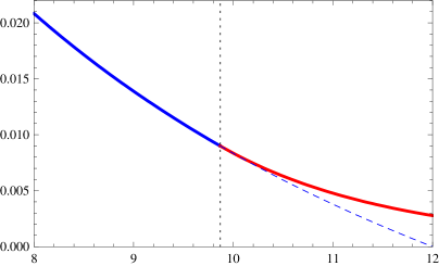
(a) $F^{\prime}(A)$

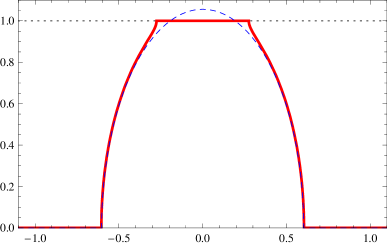
(b) Comparison of $\rho(h)$

Figure 54: Transition of the derivative of the free energy $F^{\prime}$ at $A=A_{\mathrm{crit}}=\pi^{2}$ and comparison of density functions slightly above $A_{\mathrm{crit}}$.

We can now compare the two regimes. The expansion of the derivative of the free energy around the critical point $A=A_{\mathrm{crit}}=\pi^{2}$ yields in the two cases

$$F^{\prime}_{\mathrm{rat}}\mathrel{} = \mathrel{}\frac{1}{2\pi^{2}}-\frac{1}{24}-\frac{A-A_{\mathrm{crit}}}{2\pi^{4}}+\frac{(A-A_{\mathrm{crit}})^{2}}{2\pi^{6}}-\frac{(A-A_{\mathrm{crit}})^{3}}{2\pi^{8}}+\ldots\,,$$

$$F^{\prime}_{\mathrm{ell}}\mathrel{} = \mathrel{}\frac{1}{2\pi^{2}}-\frac{1}{24}-\frac{A-A_{\mathrm{crit}}}{2\pi^{4}}+\frac{3(A-A_{\mathrm{crit}})^{2}}{2\pi^{6}}-\frac{13(A-A_{\mathrm{crit}})^{3}}{4\pi^{8}}+\ldots\,,$$ (B.11)

see Fig. 54a. The deviation is therefore of second order

$$\Delta F^{\prime}=+\frac{(A-A_{\mathrm{crit}})^{2}}{\pi^{6}}-\frac{11(A-A_{\mathrm{crit}})^{3}}{4\pi^{8}}+\ldots$$ (B.12)

implying a third-order transition in the free energy $F$.

In fact the function $u(h)$ deviates only quadratically at a generic point away from the branch points, see Fig. 54b. It can be expected that the same holds whenever an elliptic curve degenerated into a rational curve. This leads to the conclusion that all quantities which can be read off directly from the curve (e.g. in an expansion) will deviate at least quadratically.

Appendix C Integration of the Partial Filling Fractions

Analytically integrating the partial filling fractions $\alpha_{1}$, $\alpha_{2}$ of the two-cut solution (4.11) is possible because they can be expressed as integrals over A-cycles (2.23) of the derivative $\tilde{p}_{0}^{\prime}(x)$, which is an algebraic function:

$$\alpha_{1,2}\mathrel{} = \mathrel{}-\frac{1}{2\pi i}\oint_{\mathcal{A}_{1,2}}p(x)\,\mathrm{d}x$$ (C.1)

$$= \mathrel{}-\frac{1}{2\pi i}\oint_{\mathcal{A}_{1,2}}\tilde{p}_{0}\circ\mu(x)+C\,\mathrm{d}x$$

$$= \mathrel{}-\frac{1}{2\pi i}\oint_{\mathcal{A}_{1,2}}\bigl{(}(\tilde{p}_{0}+C)\circ\mu\bigr{)}(x)\,\mathrm{d}x$$

$$= \mathrel{}-\frac{1}{2\pi i}\oint_{\mu(\mathcal{A}_{1,2})}\left(\tilde{p}_{0}+C\right)(y)(\mu^{-1})^{\prime}(y)\,\mathrm{d}y$$

$$= \mathrel{}\frac{1}{2\pi i}\oint_{\mu(\mathcal{A}_{1,2})}\tilde{p}_{0}^{\prime}(x)\mu^{-1}(x)\,\mathrm{d}x$$

$$= \mathrel{}\frac{1}{2\pi i}\oint_{\mu(\mathcal{A}_{1,2})}\sqrt{\frac{a_{0}^{2}(b_{0}^{2}-x^{2})}{b_{0}^{2}(a_{0}^{2}-x^{2})}}$$

$$\mathord{}\cdot\frac{\Delta n\left(b_{0}^{2}(sx-u)^{2}\mathop{\smash{\operator@font E}\vphantom{a}}\nolimits(q)-(a_{0}^{2}s-ux)(b_{0}^{2}s-ux)\mathop{\smash{\operator@font K}\vphantom{a}}\nolimits(q)\right)}{a_{0}(rx-t)(sx-u)(b_{0}^{2}-x^{2})}\,\mathrm{d}x\,.$$

In the following, this integral will be evaluated for the case $0<a_{0}<b_{0}<\infty$. The result can then be analytically continued to the case of complex $a_{0}$ and $b_{0}=\bar{a}_{0}$. For $0<a_{0}<b_{0}<\infty$ the contours $\mathcal{A}_{1,2}$ encircle the real intervals $I_{1}:=[a_{0},b_{0}]$, $I_{2}:=[-b_{0},-a_{0}]$. Except for an overall sign, the integrand $\tilde{p}_{0}^{\prime}(x)\mu^{-1}(x)$ has the same values above and below the intervals $I_{1,2}$. Therefore, the integrals along the contours $\mathcal{A}_{1,2}$ can be expressed as integrals over $I_{1,2}$:

$$\oint\limits_{\mu(\mathcal{A}_{1,2})}\tilde{p}_{0}^{\prime}(x)\mu^{-1}(x)\,\mathrm{d}x=2\lim_{\varepsilon\rightarrow 0}\int\limits_{I_{1,2}-i\varepsilon}\tilde{p}_{0}^{\prime}(x)\mu^{-1}(x)\,\mathrm{d}x\,.$$ (C.2)

Since

$$\mathop{\mathrm{Im}}\left(\frac{b_{0}^{2}-(x-i\varepsilon)^{2}}{a_{0}^{2}-(x-i\varepsilon)^{2}}\right)\xrightarrow{\varepsilon\rightarrow 0}\begin{cases}<0&\text{for $x\in I_{1}$}\\ >0&\text{for $x\in I_{2}$}\end{cases}\,,$$ (C.3)

the square root in the integrand on the right hand side becomes

$$\sqrt{\frac{b_{0}^{2}-(x-i\varepsilon)^{2}}{a_{0}^{2}-(x-i\varepsilon)^{2}}}\xrightarrow{\varepsilon\rightarrow 0}\begin{Bmatrix}-i&(x\in I_{1})\\ i&(x\in I_{2})\end{Bmatrix}\sqrt{\frac{b_{0}^{2}-x^{2}}{x^{2}-a_{0}^{2}}}\,.$$ (C.4)

The partial filling fraction integrals can now be written as

$$\alpha_{1,2}=\pm\frac{\Delta n}{\pi b_{0}}\int_{I_{1,2}}\frac{1}{\sqrt{(x^{2}-a_{0}^{2})(b_{0}^{2}-x^{2})}}\left(A+\frac{A_{t/r}}{x-\frac{t}{r}}+\frac{A_{u/s}}{x-\frac{u}{s}}\right)\mathrm{d}x\,,$$ (C.5)

where $\alpha_{1}$ has the positive and $\alpha_{2}$ the negative sign. The constants are

$$A =\frac{u^{2}\mathop{\smash{\operator@font K}\vphantom{a}}\nolimits(q)-b_{0}^{2}s^{2}\mathop{\smash{\operator@font E}\vphantom{a}}\nolimits(q)}{rs}\,,$$

$$A_{t/r} =\frac{(a_{0}^{2}rs-tu)(b_{0}^{2}rs-tu)\mathop{\smash{\operator@font K}\vphantom{a}}\nolimits(q)-b_{0}^{2}(st-ru)^{2}\mathop{\smash{\operator@font E}\vphantom{a}}\nolimits(q)}{r^{2}(st-ru)}\,,$$

$$A_{u/s} =\frac{-(a_{0}^{2}s^{2}-u^{2})(b_{0}^{2}s^{2}-u^{2})\mathop{\smash{\operator@font K}\vphantom{a}}\nolimits(q)}{s^{2}(st-ru)}\,.$$ (C.6)

The integral (C.5) can be performed term by term. The first term is the simplest:

$$\int_{I_{1,2}}\frac{1}{\sqrt{(x^{2}-a_{0}^{2})(b_{0}^{2}-x^{2})}}\,\mathrm{d}x=\frac{1}{b_{0}}\mathop{\smash{\operator@font K}\vphantom{a}}\nolimits(q)\,.$$ (C.7)

The second and third term are of the same form, but the results for either contour differ by a sign:

$$\int_{I_{1}} \frac{1}{\sqrt{(x^{2}-a_{0}^{2})(b_{0}^{2}-x^{2})}}\frac{1}{x-c}\,\mathrm{d}x$$

$$=\int_{a_{0}}^{b_{0}}\frac{x+c}{\sqrt{(x^{2}-a_{0}^{2})(b_{0}^{2}-x^{2})}(x^{2}-c^{2})}\,\mathrm{d}x$$

$$=\frac{\pi}{2\sqrt{(a_{0}^{2}-c^{2})(b_{0}^{2}-c^{2})}}-\frac{c}{b_{0}(c^{2}-a_{0}^{2})}\left(\frac{c^{2}-a^{2}}{c^{2}}\mathop{\smash{\operator@font K}\vphantom{a}}\nolimits(q)+\frac{a_{0}^{2}}{c^{2}}\mathop{\smash{\operator@font\tilde{\Pi}}\vphantom{a}}\nolimits(c)\right),$$

$$\int_{I_{2}} \frac{1}{\sqrt{(x^{2}-a_{0}^{2})(b_{0}^{2}-x^{2})}}\frac{1}{x-c}\,\mathrm{d}x$$

$$=-\frac{\pi}{2\sqrt{(a_{0}^{2}-c^{2})(b_{0}^{2}-c^{2})}}-\frac{c}{b_{0}(c^{2}-a_{0}^{2})}\left(\frac{c^{2}-a^{2}}{c^{2}}\mathop{\smash{\operator@font K}\vphantom{a}}\nolimits(q)+\frac{a_{0}^{2}}{c^{2}}\mathop{\smash{\operator@font\tilde{\Pi}}\vphantom{a}}\nolimits(c)\right).$$ (C.8)

For obtaining these two forms, the integrals

$$\int_{a_{0}}^{b_{0}}\frac{x}{\sqrt{(x^{2}-a_{0}^{2})(b_{0}^{2}-x^{2})}(x^{2}-c^{2})}\,\mathrm{d}x =\int_{a_{0}^{2}}^{b_{0}^{2}}\frac{1}{2\sqrt{(t-a_{0}^{2})(b_{0}^{2}-t)}(t-c^{2})}\,\mathrm{d}t$$

$$=\frac{\pi}{2\sqrt{(a_{0}^{2}-c^{2})(b_{0}^{2}-c^{2})}}$$ (C.9)

and

$$\int_{a_{0}}^{b_{0}}\frac{c}{\sqrt{(x^{2}-a_{0}^{2})(b_{0}^{2}-x^{2})}(x^{2}-c^{2})}\,\mathrm{d}x=-\frac{c}{b_{0}(c^{2}-a_{0}^{2})}\left(\frac{c^{2}-a^{2}}{c^{2}}\mathop{\smash{\operator@font K}\vphantom{a}}\nolimits(q)+\frac{a_{0}^{2}}{c^{2}}\mathop{\smash{\operator@font\tilde{\Pi}}\vphantom{a}}\nolimits(c)\right)$$ (C.10)

were used. The latter can be found in [48], formula 217.12. Putting it all together and writing the occurring square roots in the form (4.17) in order to select the branch of the square root consistently, one arrives at the result (4.19).

Appendix D Integral of the Two-Cut Quasi-Momentum

In order to find the physical cut contours for a given two-cut quasi-momentum $p(x)$, one can use the fact that expression (4.22) must be real on the physical contours. That expression contains the integral of the quasi-momentum, which will be given here. Direct integration yields

$$\int^{y} \mu^{-1}(z)\tilde{p}_{0}^{\prime}(z)\,\mathrm{d}z=$$

$$-\frac{ia_{0}\Delta n}{rs(b_{0}^{2}-y^{2})}\sqrt{\frac{-1}{a_{0}^{2}}}\sqrt{\frac{a_{0}^{2}(b_{0}^{2}-y^{2})}{b_{0}^{2}(a_{0}^{2}-y^{2})}}\sqrt{1-\frac{y^{2}}{a_{0}^{2}}}\sqrt{1-\frac{y^{2}}{b_{0}^{2}}}$$

$$\mspace{100.0mu}\cdot\left(b_{0}^{2}s^{2}\mathop{\smash{\operator@font E}\vphantom{a}}\nolimits(q)-u^{2}\mathop{\smash{\operator@font K}\vphantom{a}}\nolimits(q)\right)\mathop{\smash{\operator@font F}\vphantom{a}}\nolimits\left(i\mathop{\mathrm{arsinh}}\left({\sqrt{\frac{-1}{a_{0}^{2}}}\,y}\right)\mathpunct{\Bigg{|}}1-q\right)$$

$$+\frac{4\Delta n\,a_{0}}{b_{0}^{2}}\,\frac{\displaystyle\sqrt{\frac{a_{0}(b_{0}+y)}{(a_{0}-b_{0})(y-a_{0})}}\sqrt{\frac{a_{0}(b_{0}-y)}{(a_{0}+b_{0})(a_{0}-y)}}}{\displaystyle\sqrt{\frac{(a_{0}-b_{0})(a_{0}+y)}{(a_{0}+b_{0})(a_{0}-y)}}\sqrt{\frac{a_{0}^{2}(b_{0}^{2}-y^{2})}{b_{0}^{2}(a_{0}^{2}-y^{2})}}}$$

$$\mspace{20.0mu}\cdot\Biggl{(}\frac{b_{0}^{2}(st-ru)^{2}\mathop{\smash{\operator@font E}\vphantom{a}}\nolimits(q)-(a_{0}^{2}rs-tu)(b_{0}^{2}rs-tu)\mathop{\smash{\operator@font K}\vphantom{a}}\nolimits(q)}{(a_{0}^{2}r^{2}-t^{2})(st-ru)}\mathop{\smash{\operator@font\Pi}\vphantom{a}}\nolimits_{r,t}(y)$$

$$\mspace{50.0mu}+\frac{b_{0}^{2}s^{2}-u^{2}}{st-ru}\mathop{\smash{\operator@font K}\vphantom{a}}\nolimits(q)\mathop{\smash{\operator@font\Pi}\vphantom{a}}\nolimits_{s,u}(y)$$

$$\mspace{50.0mu}-\frac{b_{0}^{2}s(st-ru)\mathop{\smash{\operator@font E}\vphantom{a}}\nolimits(q)+(a_{0}^{2}rsu-tu^{2}+a_{0}r(u^{2}-b_{0}^{2}s^{2}))\mathop{\smash{\operator@font K}\vphantom{a}}\nolimits(q)}{2a_{0}rs(a_{0}r-t)}$$

$$\mspace{140.0mu}\cdot\mathop{\smash{\operator@font F}\vphantom{a}}\nolimits\left(\arcsin\sqrt{\frac{(a_{0}-b_{0})(a_{0}+y)}{(a_{0}+b_{0})(a_{0}-y)}}\,\mathpunct{\Bigg{|}}\frac{(a_{0}+b_{0})^{2}}{(a_{0}-b_{0})^{2}}\right)\Biggr{)}\,,$$ (D.1)

where

$$\mathop{\smash{\operator@font\Pi}\vphantom{a}}\nolimits_{A,B}(x):=\mathop{\smash{\operator@font\Pi}\vphantom{a}}\nolimits\left(\frac{(a_{0}+b_{0})(a_{0}A-B)}{(a_{0}-b_{0})(a_{0}A+B)};\arcsin\sqrt{\frac{(a_{0}-b_{0})(a_{0}+x)}{(a_{0}+b_{0})(a_{0}-x)}}\,\mathpunct{\Bigg{|}}\frac{(a_{0}+b_{0})^{2}}{(a_{0}-b_{0})^{2}}\right)$$ (D.2)

and where $\mathop{\smash{\operator@font F}\vphantom{a}}\nolimits(z\mathpunct{|}q)$ is the incomplete elliptic integral of the first kind:

$$\mathop{\smash{\operator@font F}\vphantom{a}}\nolimits(z\mathpunct{|}q)=\int_{0}^{\sin z}\frac{1}{\sqrt{(1-t^{2})(1-qt^{2})}}\,\mathrm{d}t\,.$$ (D.3)

Using the integral (D.1), one can obtain a closed expression for the integral $\mathnormal{\Lambda}(x)$ of the two-cut quasi-momentum $p(x)$ (4.11), which can be expressed as

$$\mathnormal{\Lambda}(x)\mathrel{} = \mathrel{}\int^{x}p(y)\,\mathrm{d}y=xp(x)-\int^{x}yp^{\prime}(y)\,\mathrm{d}y$$ (D.4)

$$= \mathrel{}xp(x)-\int^{x}y\tilde{p}_{0}^{\prime}(\mu(y))\mu^{\prime}(y)\,\mathrm{d}y=xp(x)-\int^{\mu(x)}\mu^{-1}(z)\tilde{p}_{0}^{\prime}(z)\,\mathrm{d}z\,.$$

References

- [1] W. Heisenberg, “Zur Theorie des Ferromagnetismus”, Z. Phys. 49, 619 (1928).
- [2] H. Bethe, “Zur Theorie der Metalle I. Eigenwerte und Eigenfunktionen der linearen Atomkette”, Z. Phys. 71, 205 (1931).
- [3] V. E. Korepin, N. M. Bogoliubov and A. G. Izergin, “Quantum Inverse Scattering Method and Correlation Functions”, Cambridge University Press (1993), Cambridge, UK, 575p.
- [4] L. Hulthén, “Über das Austauschproblem eines Kristalles”, Almqvist & Wiksell (1938), Stockholm, Sweden.
- [5] L. A. Takhtajan, “The picture of low-lying excitations in the isotropic Heisenberg chain of arbitrary spins”, Phys. Lett. A87, 479 (1982).
- [6] L. D. Faddeev and L. A. Takhtajan, “What is the spin of a spin wave?”, Phys. Lett. A85, 375 (1981).
- [7] R. J. Baxter, “Completeness of the Bethe ansatz for the six and eight-vertex models”, J. Stat. Phys. 108, 1 (2002), cond-mat/0111188.
- [8] B. Sutherland, “Low-Lying Eigenstates of the One-Dimensional Heisenberg Ferromagnet for any Magnetization and Momentum”, Phys. Rev. Lett. 74, 816 (1995).
- [9] N. Beisert, J. A. Minahan, M. Staudacher and K. Zarembo, “Stringing Spins and Spinning Strings”, JHEP 0309, 010 (2003), hep-th/0306139.
- [10] A. Dhar and B. S. Shastry, “Bloch Walls and Macroscopic String States in Bethe’s solution of the Heisenberg Ferromagnetic Linear Chain”, Phys. Rev. Lett. 85, 2813 (2000), cond-mat/0005397.
- [11] J. A. Minahan and K. Zarembo, “The Bethe-ansatz for 4 super Yang-Mills”, JHEP 0303, 013 (2003), hep-th/0212208.
- [12] N. Beisert, S. Frolov, M. Staudacher and A. A. Tseytlin, “Precision Spectroscopy of AdS/CFT”, JHEP 0310, 037 (2003), hep-th/0308117.
- [13] S. Frolov and A. A. Tseytlin, “Multi-spin string solutions in ”, Nucl. Phys. B668, 77 (2003), hep-th/0304255.
- [14] S. Frolov and A. A. Tseytlin, “Rotating string solutions: AdS/CFT duality in non-supersymmetric sectors”, Phys. Lett. B570, 96 (2003), hep-th/0306143.
- [15] A. A. Tseytlin, “Spinning strings and AdS/CFT duality”, hep-th/0311139, in: “From Fields to Stings: Circumnavigating Theoretical Physics”, ed.: M. Shifman, A. Vainshtein and J. Wheater, World Scientific (2005), Singapore.
- [16] J. Plefka, “Spinning strings and integrable spin chains in the AdS/CFT correspondence”, Living. Rev. Relativity 8, 9 (2005), hep-th/0507136.
- [17] D. Berenstein, J. M. Maldacena and H. Nastase, “Strings in flat space and pp waves from 4 Super Yang Mills”, JHEP 0204, 013 (2002), hep-th/0202021.
- [18] M. Kruczenski, “Spin chains and string theory”, Phys. Rev. Lett. 93, 161602 (2004), hep-th/0311203.
- [19] E. Fradkin, “Field Theories of Condensed Matter Systems”, Addison-Wesley (1991), 350p.
- [20] R. F. Bikbaev, A. I. Bobenko and A. R. Its, “On finite-zone integration of the Landau-Lifshits equation”, Soviet Math. Dokl. 28, 512 (1983).
- [21] V. A. Kazakov, A. Marshakov, J. A. Minahan and K. Zarembo, “Classical/quantum integrability in AdS/CFT”, JHEP 0405, 024 (2004), hep-th/0402207.
- [22] B. A. Dubrovin, V. B. Matveev and S. P. Novikov, “Non-linear equations of Korteweg-De Vries type, finite-zote linear operators, and abelian varieties”, Russ. Math. Surv. 31:1, 59 (1976).
- [23] N. Beisert, A. A. Tseytlin and K. Zarembo, “Matching Quantum Strings to Quantum Spins: One-Loop vs. Finite-Size Corrections”, Nucl. Phys. B715, 190 (2005), hep-th/0502173.
- [24] S. Frolov and A. A. Tseytlin, “Quantizing three-spin string solution in ”, JHEP 0307, 016 (2003), hep-th/0306130.
- [25] N. Beisert and L. Freyhult, “Fluctuations and Energy Shifts in the Bethe Ansatz”, Phys. Lett. B622, 343 (2005), hep-th/0506243.
- [26] R. Hernández, E. López, A. Periáñez and G. Sierra, “Finite size effects in ferromagnetic spin chains and quantum corrections to classical strings”, JHEP 0506, 011 (2005), hep-th/0502188.
- [27] N. Gromov and P. Vieira, “Complete 1-loop test of AdS/CFT”, arxiv:0709.3487.
- [28] N. Gromov and V. Kazakov, “Double scaling and finite size corrections in sl(2) spin chain”, Nucl. Phys. B736, 199 (2006), hep-th/0510194.
- [29] J. A. Minahan, “Higher loops beyond the SU(2) sector”, JHEP 0410, 053 (2004), hep-th/0405243.
- [30] N. Beisert, V. Dippel and M. Staudacher, “A Novel Long Range Spin Chain and Planar 4 Super Yang-Mills”, JHEP 0407, 075 (2004), hep-th/0405001.
- [31] G. Arutyunov and M. Staudacher, “Matching Higher Conserved Charges for Strings and Spins”, JHEP 0403, 004 (2004), hep-th/0310182.
- [32] M. R. Douglas and V. A. Kazakov, “Large N phase transition in continuum QCD in two-dimensions”, Phys. Lett. B319, 219 (1993), hep-th/9305047.
- [33] N. Dorey and B. Vicedo, “On the dynamics of finite-gap solutions in classical string theory”, JHEP 0607, 014 (2006), hep-th/0601194.
- [34] N. Dorey and B. Vicedo, “A symplectic structure for string theory on integrable backgrounds”, JHEP 0703, 045 (2007), hep-th/0606287.
- [35] B. Vicedo, “Semiclassical Quantisation of Finite-Gap Strings”, arxiv:0803.1605.
- [36] S. Schäfer-Nameki, M. Zamaklar and K. Zarembo, “Quantum corrections to spinning strings in and Bethe ansatz: A comparative study”, JHEP 0509, 051 (2005), hep-th/0507189.
- [37] S. Schäfer-Nameki, “Exact expressions for quantum corrections to spinning strings”, Phys. Lett. B639, 571 (2006), hep-th/0602214.
- [38] H. Dimov and R. C. Rashkov, “A note on spin chain/string duality”, Int. J. Mod. Phys. A20, 4337 (2005), hep-th/0403121.
- [39] B. Vicedo, “Giant magnons and singular curves”, JHEP 0712, 078 (2007), hep-th/0703180.
- [40] G. Arutyunov, S. Frolov, J. Russo and A. A. Tseytlin, “Spinning strings in and integrable systems”, Nucl. Phys. B671, 3 (2003), hep-th/0307191.
- [41] G. Arutyunov, J. Russo and A. A. Tseytlin, “Spinning strings in : New integrable system relations”, Phys. Rev. D69, 086009 (2004), hep-th/0311004.
- [42] A. A. Tseytlin, “Semiclassical strings and AdS/CFT”, hep-th/0409296, in: “String Theory: from Gauge Interactions to Cosmology”, ed.: L. Baulieu, J. de Boer, B. Pioline and E. Rabinovici, Springer (2005), Berlin, Germany, 410p.
- [43] J. A. Minahan, A. Tirziu and A. A. Tseytlin, “ corrections to semiclassical AdS/CFT states from quantum Landau-Lifshitz model”, Nucl. Phys. B735, 127 (2006), hep-th/0509071.
- [44] B. Rusakov, “Large N quantum gauge theories in two-dimensions”, Phys. Lett. B303, 95 (1993), hep-th/9212090.
- [45] D. J. Gross, “Two-dimensional QCD as a string theory”, Nucl. Phys. B400, 161 (1993), hep-th/9212149.
- [46] D. J. Gross and W. Taylor, “Two-dimensional QCD is a string theory”, Nucl. Phys. B400, 181 (1993), hep-th/9301068.
- [47] D. J. Gross and W. Taylor, “Twists and Wilson loops in the string theory of two- dimensional QCD”, Nucl. Phys. B403, 395 (1993), hep-th/9303046.
- [48] P. F. Byrd and M. D. Friedman, “Handbook of Elliptic Integrals for Engineers and Scientists”, 2nd edition, Springer Verlag (1971), New York, USA, 358p.