Dynamics of symmetric dynamical systems with delayed switching

Abstract

We study dynamical systems that switch between two different vector fields depending on a discrete variable and with a delay. When the delay reaches a problem-dependent critical value so-called event collisions occur. This paper classifies and analyzes event collisions, a special type of discontinuity induced bifurcations, for periodic orbits. Our focus is on event collisions of symmetric periodic orbits in systems with full reflection symmetry, a symmetry that is prevalent in applications. We derive an implicit expression for the Poincaré map near the colliding periodic orbit. The Poincaré map is piecewise smooth, finite-dimensional, and changes the dimension of its image at the collision. In the second part of the paper we apply this general result to the class of unstable linear single-degree-of-freedom oscillators where we detect and continue numerically collisions of invariant tori. Moreover, we observe that attracting closed invariant polygons emerge at the torus collision.

Keywords: delay, relay, hysteresis, invariant torus collision

1 Introduction

Relay control systems, which can be regarded as hybrid systems, are applied in many different areas of engineering applications. Relay feedback control might involve control of stationary processes in industry as well as control of moving objects, for instance in flight control. Hence, it is not surprising that in recent years much research effort has been spent on investigations of the dynamics of relay systems characterized by idealized off/on relay control, see for instance [11, 16] among other works. However, relay systems often feature intrinsic hysteretic behavior [22] as well as delay in the control input. For instance, if we control a plant using simple on/off relay feedback control via a computer network, our control input may be delayed, due to the traffic along the network.

In the current paper we study the dynamics of relay control systems with hysteretic behavior and delay in the control input. We wish to understand if and how the interplay between the discontinuous nonlinearities (switching events), hysteresis and delay in the switching function can lead to new bifurcations. We expect so-called event-collisions to occur as observed in [7]. We show that they cause a change in the dimension of the phase space that describes the local dynamics of the system, which leads to interesting dynamical phenomena such as closed invariant polygons and collisions of smooth invariant tori.

Let us explain the problem for the classical prototype example of an oscillator subject to a relay switch:

$$\ddot{x}+\zeta\dot{x}+\omega^{2}x=u\mbox{.}$$ (1)

This example will be studied in detail in Section 5 and in Section 6. In (1) $y=[x,\dot{x}]^{T}$ is the continuous variable and $u$ provides discrete feedback in the form of a relay. That is, $u$ is ruled by the switching law:

$$u(t)=\begin{cases}\mp 1&\mbox{if $\pm h^{T}y(t-\tau)\geq\varepsilon$}\\ \lim_{s\nearrow t}u(s)&\mbox{if $h^{T}y(t-\tau)\in(-\varepsilon,\varepsilon)$.}\end{cases}$$ (2)

Roughly speaking, the switching law (2) means that we set $u$ to $-1$ whenever we observe that $h^{T}y\geq\varepsilon$ and we set $u$ to $+1$ whenever we observe that $h^{T}y\leq-\varepsilon$ (negative feedback). The region $\{|h^{T}y|<\varepsilon\}$ provides a hysteresis in the relay (a buffer between subsequent switchings from $u$ to $-u$): we leave $u$ at its value when we observe that $|h^{T}y|<\varepsilon$. The lines $\{y:h^{T}y=\pm\varepsilon\}$ are called the switching lines or, more generally for higher dimensional $y$ and nonlinear switching functions $h$, switching manifolds. An ordinary differential equation such as (1) with a switching law of the form (2) is one of the simplest forms of hybrid dynamical systems [21]. The twist in problem (1), (2) comes from the presence of a delay $\tau$ in the observation (or the switching) in (2). Figure 1 illustrates how a trajectory of (1) might look like. The presence of a small delay $\tau$ is often equivalent to a perturbation of the switching law (only if $\varepsilon$ is positive, see, for example, [7]). For large delays $\tau$ the dynamics shows an enormous amount of complexity [4, 5, 7, 15] because the number of switching times in the interval $[t-\tau,t]$ is effectively included into the dimension of the system which then becomes larger than the dimension of the physical space [27].

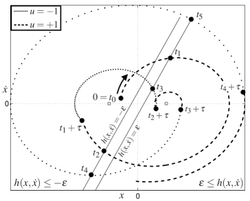
Figure 1: Sketch of qualitative behavior of hybrid systems with delay. Initial history segment of $(x,\dot{x})$ is assumed to be constant, initial value of $u$ is $+1$. The solid lines are the switching manifolds $h=\pm\varepsilon$. At the times $t_{j}$ the trajectory crosses the switching line, at the times $t_{j}+\tau$ it switches the control $u$ to $-u$.

This paper studys the transition from ‘small’ to ‘large’ delay. This transition is characterized by event collisions, which are discontinuity induced bifurcations [7]. The notion of a discontinuity induced bifurcation can be made precise for periodic orbits of (1), (2). The possible types of codimension one discontinuity induced bifurcations for generic systems with delayed switching have been classified and analyzed in [27] (without hysteresis):

1. (grazing) the periodic orbit touches the switching manifold quadratically without intersecting it,

2. (corner/event collision) the continuous variable $y$ is on the switching manifold at two times with difference equal to the delay $\tau$: say, at time $t$ and time $t-\tau$. The name is due to the fact that the periodic orbit typically has a ‘corner’ at $t$ because it switches the vector field ($u\mapsto-u$) at $t$.

Most of the event collisions reported in [7] violate one of the secondary genericity conditions in [27], namely that only one corner collides. The reason behind this unexpected degeneracy of the phenomena observed in [7] is that the oscillator system (1), (2) (which is the subject of study in [7]) is symmetric with respect to reflection at the origin:

$$y\mapsto-y\mbox{,\quad}u\mapsto-u\mbox{.}$$ (3)

The periodic orbits of primary interest inherit this symmetry. If the control switches from $u$ to $-u$ at time $t$ it switches from $-u$ to $u$ one half-period later (at $t+p/2$ if $p$ is the period). Whenever the corner at $t$ is on the switching manifold the opposite corner (at $t+p/2$) is on the switching manifold as well due to reflection symmetry. This is in contrast to the secondary genericity conditions in [27]. In fact, all systems studied in [4, 5, 7, 15] have a reflection symmetry because they are piecewise linear, which renders the generic theory inapplicable to symmetric periodic orbits in these examples of practical interest.

We close this gap in the general context, that is, for $y\in\mathbb{R}^{n}$ and nonlinear right-hand-sides and switching laws. The first main result of the paper is an implicit expression for the local return map for symmetric periodic orbits close to a simultaneous collision of two corners. The simplest example for this scenario is a symetric periodic orbit of period $p=2\tau$ for which $y(0)$ and $y(\tau)$ lie both on the switching manifold. Due to the reflection symmetry this event has codimension one. The return map near a colliding orbit is a piecewise smooth map $F$ that has a $(n-1)$-dimensional image in one subdomain of its phase space and a $n$-dimensional image in the other subdomain. This type of map has been studied extensively in the context of grazing bifurcations in Filippov systems (systems where $\varepsilon=\tau=0$; see the textbook [9] and the recent review [18]). In this sense our paper provides a link between the theory of systems with delayed switching and hysteresis to the theory of low-dimensional piecewise smooth maps as treated in [9].

The second aspect of the paper is a study of the concrete class of oscillators (1), (2) near event collisions of symmetric periodic orbits. We pay special attention to parameter regimes where the event collision leads to quasi-periodicity and, thus, collisions of invariant tori and the appearance of closed invariant polygons. None of the phenomena described in the sections 5 and 6 are present in [7] because the authors restricted their study to the special case of pure position feedback $h^{T}=(1,0)$ in the switching law (2).

The first part of our paper adopts a ‘local’ approach, which is slightly different from the studies [4, 5, 7, 14, 15]. We do not aim to classify the dynamics of a particular class of systems as completely as possible. Instead, we develop a local bifurcation theory, considering a general system with $n$-dimensional physical space and assuming that it has a periodic orbit $(y_{*},u_{*})$. Then we study the dynamics near the periodic orbit deriving conditions for the presence of bifurcations of a certain codimension. In this way our results will be more general than studies of specific classes of systems but all statements are valid only locally. The consideration of only two vector fields and and a binary switch is not really a restriction when one studies the local dynamics near a particular periodic orbit. The second part of the paper then demonstrates how this local bifurcation theory can be useful in combination with numerical continuation to understand the dynamics of the class of oscillators (1), (2).

The paper is organized as follows. In Section 2 we introduce the basic notation and collect some fundamental facts about the forward evolution defined by general systems with delayed switching and hysteresis. We also point out differences to the neighboring cases of zero hysteresis or zero delay. Section 3 specifies conditions on periodic orbits which guarantee that a local return map exists and that this map is finite-dimensional and, generically, smooth. Section 4 classifies and analyzes the codimension one discontinuity induced bifurcations of periodic orbits for systems with reflection symmetry. Section 5 studys the single-degree-of-freedom oscillator (1), (2) near an event collision, classifying the local bifurcations of symmetric periodic orbits. In Section 6 we unfold the collision of a Neimark-Sacker bifurcation with the switching line, a codimension two event involving collisions of closed invariant curves and closed invariant polygons. The appendix contains the proofs of all lemmas and the technical details of some constructions.

2 Fundamental properties of the evolution

We consider general hybrid dynamical systems with delay of the following form:

$$\dot{y}(t) = f(y(t),u(t))$$ (4)

$$u(t) = \begin{cases}-1&\mbox{if $h(y(t-\tau))\geq\varepsilon$, or}\\ &\mbox{if $h(y(t-\tau))\in(-\varepsilon,\varepsilon)$ and $u_{-}(t)=-1$,}\\ \phantom{-}1&\mbox{if $h(y(t-\tau))\leq-\varepsilon$, or}\\ &\mbox{if $h(y(t-\tau))\in(-\varepsilon,\varepsilon)$ and $u_{-}(t)=1$}\\ \end{cases}$$ (5)

where $\varepsilon$ is positive. The continuous variable $y$ is $n$-dimensional and the discrete variable $u$ is, for simplicity of presentation, binary, controlling the switching between the two vector fields $Y_{\pm}^{t}$ given by $\dot{y}=f(y,\pm 1)$. In the definition of $u(t)$ in (5), $u_{-}(t)$ is defined as

$$u_{-}(t):=\lim_{s\nearrow t}u(s)\mbox{.}$$ (6)

We assume continuous differentiability for the functions $f(\cdot,\pm 1):\mathbb{R}^{n}\mapsto\mathbb{R}^{n}$ and $h:\mathbb{R}^{n}\mapsto\mathbb{R}$ in the right-hand-side of (4), (5) with respect to the argument $y$ (and, possibly, parameters). Furthermore, we assume that the gradient $h^{\prime}$ is non-zero everywhere and that $f$ and $h$ have uniform Lipschitz constants (using a prime for the derivative with respect to $y$):

$$\|f^{\prime}\|\leq L_{\max}\mbox{, and\ }\|h^{\prime}\|\leq H_{\max}\mbox{.}$$

Due to the delay in the argument of $y$ in the switching decision (5) the phase space of (4), (5) is infinite-dimensional. An appropriate initial value for $y$ is the history segment $y([-\tau,0])$ [12, 29]. Thus, the phase space of (4), (5) is $C([-\Theta,0];\mathbb{R}^{n})\times\{-1,1\}$ where $\Theta$ is an upper bound for the delay $\tau$ (we will vary $\tau$ as a bifurcation parameter in the sections 5 and 6). The notation $C([-\Theta,0];\mathbb{R}^{n})$ refers to the space of continuous functions on the interval $[-\Theta,0]$ with values in $\mathbb{R}^{n}$.

We clarify in Appendix A in which sense system (4), (5) constitutes a dynamical system. In particular, we give a precise definition of the forward evolution $E^{t}(\xi,u_{0})$ from an arbitrary initial condition $(\xi_{0},u_{0})\in C([-\Theta,0];\mathbb{R}^{n})\times\{-1,1\}$ using the variation of constants formulation of (4), (5). The evolution $E^{t}(\xi_{0},u_{0})$ has a continuous infinite-dimensional component $E_{c}^{t}(\xi_{0},u_{0})\in C([-\Theta,0];\mathbb{R}^{n})$ and a discrete component $E_{d}^{t}(\xi_{0},u_{0})\in\{-1,1\}$. The infinite-dimensional components are related to each other by a simple time shift:

$$E_{c}^{t}(\xi_{0},u_{0})(\theta)=E_{c}^{t+\theta}(\xi_{0},u_{0})(0)$$

with a common headpoint trajectory $E_{c}^{t}(\xi_{0},u_{0})(0)\in C([0,t_{E}];\mathbb{R}^{n})$ for all $\theta\in[-\Theta,0]$ and $t\in[0,t_{E}]$; see [12]. Thus, $E_{c}^{t}(\xi_{0},u_{0})$ is continuous in $t$ for all $t\geq 0$. However, in general $E_{c}^{t}(\xi_{0},u_{0})$ (for a fixed $t$) does not depend continuously on the component $\xi_{0}$ of its initial value.

Lemma 1 summarizes two basic facts about the evolution $E^{t}(\xi,u)$ that are proved in Appendix A.

Lemma 1 (Fundamental properties of evolution)

Let $E^{t}(\xi_{0},u_{0})$ be a trajectory of the dynamical system (4), (5) on a bounded interval $[t_{0},t_{E}]$. Then the following holds.

1. The discrete component $E_{d}^{t}(\xi_{0},u_{0})$ changes its value (switches) only finitely many times in $[t_{0},t_{E}]$. Thus, $E_{c}$ follows either $Y_{+}$ or $Y_{-}$ for all but finitely many times $t\in[t_{0},t_{E}]$.

2. If $t_{0}\geq\tau$ then the number $n_{s}$ of switchings of $E_{d}$ is bounded by

   $$n_{s}\leq 1+[t_{E}-t_{0}]\cdot L_{\max}H_{\max}y_{\max}/(2\varepsilon)$$

   where $y_{\max}$ is the maximum of $\|E_{c}^{t}(\xi_{0},u_{0})|_{t\in[t_{0},t_{E}]}\|$ and $L_{\max}$ and $H_{\max}$ are the Lipschitz constants of $f$ and $h$, respectively.

The statements in Lemma 1 are subtly dependent on the presence of hysteresis and delay, which can be seen from the fact that statement 1 is not true in general if $\varepsilon=0$. See [27] for details about systems with switches that have delay but no hysteresis and [4, 5] for studies of a piecewise linear oscillator with rather intricate behavior.

Lemma 1 implies that the headpoint trajectory $E_{c}^{t}(\xi_{0},u_{0})(0)$ is differentiable with respect to time $t$ in any bounded interval $[t_{0},t_{E}]$, following one of the flows $Y_{\pm}$, except in a finite number of times.

3 Periodic orbits

If the relay is used to control a linearly unstable system, such as the oscillator in (1) with negative damping $\zeta$, we cannot expect to have stable equilibria. In this case the simplest possible long-time behavior of (1) is periodic motion. We focus on the dynamics near periodic orbits for the remainder of the paper. This section introduces the necessary notation and collects some basic facts about the behavior of the general relay system (4), (5) near a periodic orbit.

Definition 2 (Crossing time)

Let $L=(y_{*}(t),u_{*}(t))$ be a periodic solution of the general relay system (4), (5), that is, $y_{*}(t+p)=y_{*}(t)$, $u_{*}(t+p)=u_{*}(t)$ for all $t\geq 0$ and some period $p>0$. We call a time $t$ crossing time of $L$ if $|h(y_{*}(t))|=\varepsilon$ and $u_{*,-}(t+\tau)=\lim_{s\nearrow t}u_{*}(s+\tau)\neq u_{*}(t+\tau)$.

Equivalently, we could say that $t$ is a crossing time if $h(y_{*}(t))=\varepsilon u_{*,-}(t+\tau)=\varepsilon\lim_{s\nearrow t}u_{*}(s+\tau)$. Time $\tau$ after a crossing time $u_{*}$ will switch. A periodic orbit $L$ can have only finitely many crossing times $t_{k}$ ($k=1,\ldots,m$) per period. Thus, $L$ is differentiable, following one of the flows $Y_{\pm}$, in all times except, possibly, in $t_{k}+\tau+jp$ ($k=1,\ldots,m$, $j\in\mathbb{Z}$). We assume that the period $p$ is larger than the delay $\tau$ (without loss of generality because $p$ does not have to be the minimal period).

First, we establish when the evolution is continuous with respect to its initial value in a periodic orbit. We call the condition for continuity weak transversality. As the name suggests it excludes that the periodic orbit touches the switching manifold without crossing it (but does not require positive speed of crossing, thus, weak transversality). If this condition is satisfied then it makes sense to define a local return (or Poincaré) map along the orbit

Definition 3 (Weak transversality)

Let $L=(y_{*}(t),u_{*}(t))$ be a periodic solution of period $p$ of the general relay system (4), (5). We say that $L$ satisfies weak transversality if $|h(y_{*}(t))|$ is locally strictly monotone increasing near all crossing times $t_{1},\ldots,t_{m}\in[0,p]$ of $L$.

Weak transversality permits that $\lim_{s\nearrow t}\dot{y}_{*}(s)\neq\lim_{s\searrow t}\dot{y}_{*}(s)$ and each of the limits may be tangential to the switching manifold $\{h=\pm\varepsilon\}$ in any crossing time $t$ of $L$. However, it enforces that the periodic orbit $L$ cannot just touch the switching manifold quadratically, and that the number $m$ of crossing times is even. Weak transversality is generically satisfied for a periodic orbit.

Lemma 4 (Continuity)

If a periodic orbit $L=(y_{*}(t),u_{*}(t))$ is weakly transversal then the continuous component $E_{c}^{t}(\xi,u)$ of the evolution $E$ is continuous with respect to $\xi$ in $(\xi,u)=(y_{*}(\cdot),u_{*}(0))$ for all $t\geq 0$.

(See Appendix A for proof.) Due to this continuity it makes sense to define a local return map (also called Poincaré map) along a weakly transversal periodic orbit $L=(y_{*}(t),u_{*}(t))$ to a local cross section ${\cal S}$. Assume (without loss of generality) that neither $0$ nor $-\tau$ is a crossing time of $L$ and that $y_{*}$ follows $Y_{+}$ near time $0$ (thus, $u_{*}(0)=1$). Then $y_{*}$ is differentiable in $0$. Let $\Sigma=\{y\in\mathbb{R}^{n}:\dot{y}_{*}(0)^{T}[y-y_{*}(0)]=0\}$ be the hyperplane in $\mathbb{R}^{n}$ orthogonal to $\dot{y}_{*}(0)$ in $y_{*}(0)$. We choose as Poincaré section

$${\cal S}\!=\!\{(\xi,u)\in C([-\Theta,0];R^{n})\times\{-1,1\}:\xi(0)\in\Sigma\mbox{,\, }u=1\}\mbox{.}$$ (7)

It is not actually necessary to choose $\Sigma$ orthogonal to $\dot{y}_{*}(0)$. Any cross-section $\Sigma$ which is transversal to $y_{*}$ at $t=0$ is admissible. Let $-\tau<t_{*,1}<\ldots<t_{*,\mu}<0<t_{*,\mu+1}<\ldots<t_{*,m}<p-\tau$ be the crossing times of $L$ in $[-\tau,p-\tau]$. The following lemma states that the local return map to ${\cal S}$ is in fact a map in $\Sigma\times\mathbb{R}^{\mu}$ (a space of dimension $n-1+\mu$). The notation $U(v)$ refers to a (sufficiently small) neighborhood of a vector or number $v$ in Lemma 5 and throughout the paper.

Lemma 5 (Finite-dimensional Poincaré map)

There exist a $\delta>0$ and neighborhoods $U_{1}(y(\cdot))\subseteq U_{2}(y(\cdot))\subset C([-\Theta,0];R^{n})$ and $U(p)\subset\mathbb{R}$ such that the following holds: All initial conditions $(\xi,u)\in{\cal S}_{1}={\cal S}\cap[U_{1}(y(\cdot))\times\{1\}]$ have a unique return time $T(\xi)\in U(p)$ to ${\cal S}_{2}={\cal S}\cap[U_{2}(y(\cdot))\times\{1\}]$. For any initial condition in $(\xi,u)\in U_{1}(y(\cdot))\times\{1\}$ there exist unique times $t_{1}<\ldots<t_{\mu}$ in $(-\tau,0)$ such that

$$t_{j}=\min\{t\in[t_{*,j}-\delta,t_{*,j}+\delta]:|h(\xi(t))|=\varepsilon\}\mbox{,\quad($j=1,\ldots,\mu$).}$$ (8)

The local return map

$$P(\xi)=E^{T(\xi)}(\xi,1)$$

depends only on $(\xi(0),t_{1}\ldots,t_{\mu})\in\Sigma\times\mathbb{R}^{\mu}$.

We have omitted the discrete component of the return map from $P$ because it is always $+1$. An equivalent definition of $t_{j}$ is $t_{j}=\min\{t\in[t_{*,j}-\delta,t_{*,j}+\delta]:h(\xi(t))=\varepsilon u_{j}\}$ where $u_{j}=u_{*,-}(t_{*,j}+\tau)$. The precise dependence of $P$ on $(\xi(0),t_{1},\ldots,t_{\mu})$ is given in Appendix A.

Corollary 6 (Smooth Poincaré map for generic periodic orbits)

Assume that all crossing times $t_{*,k}$ ($k=1,\ldots,m$) of the periodic orbit $L=(y_{*},u_{*})$ satisfy the following two conditions:

1. (no collision) the time $t_{*,k}-\tau$ is a not a crossing time of $L$, and

2. (smooth transversality) $h^{\prime}(y_{*}(t_{*,k}))\,\dot{y}_{*}(t_{*,k})\neq 0$.

Then the Poincaré map $P$ depends smoothly on the coordinates $(\xi(0),t_{1},\ldots,t_{\mu})\in\Sigma\times\mathbb{R}^{\mu}$ of $(\xi,u)\in{\cal S}_{1}$ ($t_{1},\ldots,t_{\mu}$ as defined by (8)).

The two conditions of Corollary 6 guarantee that whenever $u_{*}(t)$ changes its value then $y_{*}(t-\tau)$ follows one of the two flows $Y_{\pm}$ in a neighborhood of $t-\tau$ and $\dot{y}_{*}(t-\tau)$ points transversally through the switching manifold $\{h=\pm\varepsilon\}$. Generically, these two conditions are satisfied, which implies that, generically, the Poincaré map of a periodic orbit is smooth. Condition 2 is more restrictive than weak transversality as it requires differentiability of $y_{*}(\cdot)$ and a non-zero time derivative of $h(y_{*}(\cdot))$ in $t_{*,k}$.

Corollary 6 implies that the dynamics and possible bifurcations near a periodic orbit $(y_{*},u_{*})$ of the general delayed relay system are described by the theory for low-dimensional smooth maps whenever the conditions 1 and 2 are satisfied. See, for example, [20] for a comprehensive textbook on bifurcation theory for smooth systems.

Definition 7 (Slowly oscillating periodic orbit)

We call a periodic orbit $L=(y_{*},u_{*})$ slowly oscillating if the distance between subsequent crossing times $t_{k}$ of $L$ is always greater than the delay $\tau$.

If we choose the Poincaré section ${\cal S}$ appropriately then the local return map of a slowly oscillating periodic orbit $L$ satisfying the genericity conditions of Corollary 6 is simply a return map to $\Sigma$, the hyperplane of $\mathbb{R}^{n}$ in the definition of ${\cal S}$. This has been observed in [7] for the oscillator (1), (2).

4 Discontinuity induced bifurcations

Let us assume that the right-hand-side $f$ and the switching function $h$ depend on an additional parameter $\lambda$. What happens to the dynamics near a periodic orbit under variation of $\lambda$ (or, alternatively, the delay $\tau$)? The previous section has established that, as long as the conditions of Corollary 6 are satisfied, we should expect standard bifurcation scenarios such as period doubling, saddle-node or Neimark-Sacker bifurcations (see [20] for a classification). However, when varying the parameter $\lambda$ we can also achieve that any of the conditions 1 and 2 fails at special parameter values. We call these events discontinuity induced bifurcations.

For compactness of presentation we assume that for $\lambda<\lambda_{0}$ the periodic orbit $L=(y_{*},u_{*})$ is slowly oscillating, that is, the distance between subsequent crossing times $t_{k}$ is always greater than the delay $\tau$ for $\lambda<\lambda_{0}$.

4.1 Generic bifurcations

Generic grazing

If condition 2 of Corollary 6 is violated at $\lambda=\lambda_{0}$ the orbit $L$ grazes the switching manifold tangentially at a crossing time $t_{*}$. Let us assume that $y_{*}$ follows $Y_{+}$ in $t_{*}$ without loss of generality. That is,

$$0=\frac{d}{dt}h(y_{*}(t),\lambda_{0})|_{t=t_{*}}=h^{\prime}(y_{*}(t_{*}),\lambda_{0})\,\dot{y}_{*}(t_{*})=h^{\prime}(y_{*}(t_{*}),\lambda_{0})\,f(y_{*}(t_{*}),+1,\lambda_{0})\mbox{.}$$

Generically, one can expect that

$$0\neq\frac{d^{2}}{(dt)^{2}}h(y_{*}(t),\lambda_{0})|_{t=t_{*}}=h^{\prime}(y_{*}(t_{*}),\lambda_{0})\,\ddot{y}_{*}(t_{*})+h^{\prime\prime}(y_{*}(t_{*}),\lambda_{0})\,[\dot{y}_{*}(t_{*})]^{2}\mbox{,}$$ (9)

which means that the periodic orbit $L$ touches the switching manifold quadratically and not to a higher order. However, under condition (9) $L$ is not weakly transversal. In general, we cannot expect that the evolution is continuous in $L$. Thus, trajectories arbitrarily close to $L$ leave a fixed neighborhood of $y_{*}$ in a finite time (typically one period). Consequently, generic grazing of the periodic orbit $L$ cannot be described by the approach of local bifurcation theory adopted in this paper.

Generic corner collision

If condition 2 of Corollary 6 is violated at $\lambda=\lambda_{0}$ the orbit $L$ switches between the two vector fields exactly at a crossing time $t_{1}$. That is,

$$u_{*}(t_{1})\neq\lim_{s\nearrow t_{1}}u_{*}(s)=u_{*,-}(t_{1})\mbox{.}$$

Let us denote $f_{1}=f(y_{*}(t_{1}),u_{*,-}(t_{1}),\lambda_{0})$ and $f_{2}=f(y_{*}(t_{1}),u_{*}(t_{1}),\lambda_{0})$. Generically, we can expect that

1. all other crossing times $t_{2},\ldots,t_{m}$ of $L$ do not collide, that is, $u_{*}(t_{k})=u_{*,-}(t_{k})$ for $k=2,\ldots,m$, and

2. the left-sided tangent $f_{1}$ and the right-sided tangent $f_{2}$ to $y_{*}(\cdot)$ in $t_{1}$ are transversal to the switching manifold. More precisely,

   $$q:=h^{\prime}(y_{*}(t_{1}),\lambda_{0})\,f_{1}\cdot h^{\prime}(y_{*}(t_{1}),\lambda_{0})\,f_{2}\neq 0\mbox{.}$$ (10)

If $q<0$ in condition (10) the periodic orbit $L$ has a corner at $t_{1}$ and this corner touches the switching manifold from one side at the crossing time $t_{1}$. Thus, $L$ is not weakly transversal to the switching manifold in its crossing time $t_{1}$. In this case we cannot expect that the evolution is continuous in $L$. Consequently, corner collisions with $q<0$ cannot be described using local bifurcation theory, either. An explicit expression for the return map (which is a piecewise asymptotically linear $(n-1)$-dimensional map) under the assumptions C1 and C2 for the case $q>0$ has been derived in [27] (as case (a) in Appendix D of [27]).

4.2 Corner collision with reflection symmetry

Often the practically relevant examples have special symmetries which enforce that if one corner of a symmetric periodic orbit collides at $\lambda=\lambda_{0}$ then other corners of the symmetric periodic orbit collide at $\lambda_{0}$ simultaneously. For example, the systems studied in [4, 5, 7, 15] and our prototype oscillator (1) are all piecewise affine:

$$\begin{split}f(y,u)&=Ay+bu\\ h(y)&=h^{T}y\mbox{.}\end{split}$$ (11)

Thus, they have a full reflection ($\mathbb{Z}_{2}$) symmetry

$$\begin{split}f(y,u,\lambda)&=-f(-y,-u,\lambda)\\ h(y,\lambda)&=-h(-y,\lambda)\mbox{.}\end{split}$$ (12)

This means that, even though condition C1 should be generically satisfied for a colliding periodic orbit, restricting to the generic case disregards many practically relevant systems.

The $\mathbb{Z}_{2}$ symmetry (12) typically gives rise to a symmetric periodic orbit $L=(y_{*},u_{*})$ satisfying $y_{*}(t-T)=-y_{*}(t)$ and $u_{*}(t-T)=-u_{*}(t)$ for the half-period $T$ and all times $t$. A corner collision of $L$ for a crossing time $t$ at a special parameter $\lambda=\lambda_{0}$ automatically induces a corner collision for the crossing time $t-T$, a scenario that is not covered by the generic bifurcation scenarios listed in Section 4.1.

Let us assume that system (4), (5) has full reflection symmetry (12) and a symmetric periodic orbit $L=(y_{*},u_{*})$ of half-period $T$ that experiences a corner collision at the parameter $\lambda=\lambda_{0}$ for crossing time $0$ and, enforced by symmetry, for crossing time $T$. For compactness of presentation let us assume that $0$ and $T$ are the only crossing times of $L$. This implies that the delay $\tau$ equals the half-period $T$ and that $u_{*}$ switches between $+1$ and $-1$ at the crossing times $0$ and $T$. Without loss of generality $L$ consists of the two segments

$$y_{*}([0,T])\phantom{2} =Y_{+}^{[0,T]}y_{*}(0)\mbox{,\quad} u_{*}([0,T))\phantom{2} =+1$$

$$y_{*}([T,2T]) =Y_{-}^{[0,T]}y_{*}(T)=-Y_{+}^{[0,T]}y_{*}(0) \mbox{,\quad}u_{*}([T,2T)) =-1$$

Moreover, $h(y_{*}(0),\lambda_{0})=\varepsilon$ and $h(y_{*}(T),\lambda_{0})=-\varepsilon$. Note that the colliding orbit $L$ is always following the ‘wrong’ flow. That is, the orbit is identical in shape to the periodic solution with positive feedback ($+1$ and $-1$ interchanged in (5)) and zero delay. In addition we assume that condition C2 is satisfied for the collision time $t=0$ (and, by symmetry, for $t=T$) with $q>0$. We call this condition strict transversality because it is stronger than the weak transversality introduced in Section 3:

$$q:=h_{0}^{\prime}\,f_{1}\cdot h_{0}^{\prime}f_{2}>0$$ (13)

where $h_{0}^{\prime}=h^{\prime}(y_{*}(0),\lambda_{0})$, $f_{1}=f(y_{*}(0),-1,\lambda_{0})$ and $f_{2}=f(y_{*}(0),1,\lambda_{0})$.

This strict transversality guarantees that the evolution of the continuous component $E_{c}^{t}(\xi,u)$ is continuous for $\xi=y_{*}(s+\cdot)$ for all $s\in\mathbb{R}$. We choose a cross section $\Sigma$ for the Poincaré map at $t=\Delta$ ($0<\Delta\ll 1$) and orthogonal to $f_{2}$: $\Sigma=\{y:f_{2}^{T}[y-y_{*}(\Delta)]=0\}$. If $\Delta$ is sufficiently small then $\Sigma$ is transversal to $y_{*}$ in $t=\Delta$ because $\dot{y}_{*}(\Delta)=f_{2}+O(\Delta)$.

Using the cross-section $\Sigma$ in the definition of the Poincaré map $P$, Lemma 5 states that the return map $P$ in its domain of definition

$${\cal S}_{1}=U(y_{*}(\Delta+\cdot))\cap\{\xi\in C([-\Theta,0];\mathbb{R}^{n}):\xi(0)\in\Sigma\}$$

depends for an initial value $\xi\in{\cal S}_{1}$ only on the headpoint $\xi(0)\in\Sigma$ and the time $t_{1}(\xi)=\min\{t\in[-2\Delta,0]:h(\xi(t))=\varepsilon\}$. The time $t_{1}(\xi)$ is the time when $\xi$ crosses the switching manifold $\{h=\varepsilon\}$ for the first time in $[-2\Delta,0]$. This time $t_{1}(\xi)$ exists if $U(y_{*}(\Delta+\cdot))$ is sufficiently small. Effectively, the map $P$ depends only on $n$ coordinates.

The following lemma simplifies the representation of the Poincaré map $P$ to a map from $U(y_{*}(0))$ back to $U(y_{*}(0))$.

Lemma 8 (Return map near collision)

All elements $\xi$ of the image $\operatorname{rg}P$ of the return map $P$ have the form

$$\begin{split}\xi(s)&=\begin{cases}Y_{+}^{[s+\theta(y)]}y&\mbox{if $s\in[-\theta(y),0]$,}\\ Y_{-}^{[s+\theta(y)]}y&\mbox{if $s\in[-\Theta,-\theta(y)]$,}\end{cases}\end{split}$$ (14)

where $y\in U(y_{*}(0))$ and $\theta(y)$ is implicitly defined by the condition $Y_{+}^{\theta(y)}y\in\Sigma\mbox{.}$ The coordinates $(\xi(0),t_{1}(\xi))$, which are necessary for the definition of $P$, are uniquely defined by $y$.

(See Appendix B for the proof.) We have omitted the discrete variable $u$ as an argument of $P$ because it is always $+1$ at the cross-section. The point $y=\xi(-\theta(y))$ is the point where the continuous component $\xi\in\operatorname{rg}P$ switches from following $Y_{-}$ to following $Y_{+}$. The time $\theta(y)$ is the time that has elapsed between the switching and the intersection of the headpoint with $\Sigma$. For a sufficiently small $U(y_{*}(\Delta+\cdot)$ we can assume that $\theta(y)$ is in $[0,2\Delta]$. Lemma 8 states that the return map $P$, restricted to its image $\operatorname{rg}P$, can be described as a map from the switching point of the initial value to the switching point of its image under $P$.

Exploiting the representation (14) we can describe the dynamics of the Poincaré map $P$ by a map $m$ mapping from $U(y_{*}(0))\subset\mathbb{R}^{n}$ back to $U(y_{*}(0))$.

Theorem 9 (Reduced return map near collision)

Let $\lambda$ be sufficiently close to $\lambda_{0}$. The return map $m$ for elements of the image $\operatorname{rg}P$ of the Poincaré map $P$ is given by $m=F\circ F$ where $F:U(y_{*}(0))\mapsto U(y_{*}(0))$ is defined by

$$F(y)=-Y_{+}^{\tau+t(y)}y$$ (15)

and $t(y)\in(-\Delta,\Delta)$ is the unique time such that

$$\begin{split}\varepsilon&=h\left(Y_{-}^{\,t(y)}y\right)\mbox{\quad if $h(y)\geq\varepsilon$,}\\ \varepsilon&=h\left(Y_{+}^{\,t(y)}y\right)\mbox{\quad if $h(y)<\varepsilon$.}\end{split}$$ (16)

The expression (16) of the traveling time $t(y)$ implies that $F$ is continuous in $U(y_{*}(0))$ and smooth in each of its two subdomains

$$\begin{split}D_{-}&=U(y_{*}(0))\cap\{y:h(y)\geq\varepsilon\}\mbox{\quad and}\\ D_{+}&=U(y_{*}(0))\cap\{y:h(y)<\varepsilon\}\end{split}$$ (17)

but, in general, its derivative has a discontinuity along the boundary $D_{0}$ between $D_{-}$ and $D_{+}$. The regularity of the implicit expression (16) for $t(y)$ for all $y\in U(y_{*}(0))$ follows from the strict transversality (13) of the colliding periodic orbit $L$. Let us denote the two smooth parts of the map $F$ by $F_{+}$ and $F_{-}$:

$$\begin{split}F_{+}(y)&=-Y_{+}^{\tau+t_{+}(y)}y\mbox{\quad where\quad}h\left(Y_{+}^{t_{+}(y)}y\right)=\varepsilon\mbox{, and}\\ F_{-}(y)&=-Y_{+}^{\tau+t_{-}(y)}y\mbox{\quad where\quad}h\left(Y_{-}^{t_{-}(y)}y\right)=\varepsilon\mbox{.}\end{split}$$ (18)

That is, $F|_{D_{+}}=F_{+}$ and $F|_{D_{-}}=F_{-}$. Due to the regularity of the definition of $t_{\pm}(y)$ in $U(y_{*}(0))$ the maps $F_{\pm}$ can both be extended to the whole domain $D$. The map $F_{+}$ projects $D$ nonlinearly onto the local submanifold (the delayed switching manifold)

$$\operatorname{rg}F_{+}=-Y_{+}^{\tau}[\{h=\varepsilon\}\cap U(y_{*}(0))]=\{y\in U(y_{*}(0)):h(Y_{+}^{-\tau}[-y])=\varepsilon\}\mbox{,}$$

which has co-dimension one. The linearizations of $F_{\pm}$ with respect to $y$ and the delay $\tau$ in $y=y_{*}(0)$ are

$$\begin{split}F_{\pm}(y_{*}(0)+\eta;\tau+\theta)&=y_{*}(0)-A(\tau)\left[\left[I-\frac{f_{2}h_{0}^{\prime}}{g_{\pm}}\right]\eta+\theta f_{2}\right]+O(|(\eta,\theta)|^{2})\\ g_{-}&=h_{0}^{\prime}f_{1}=-h_{0}^{\prime}A^{\tau}f_{2}\\ g_{+}&=h_{0}^{\prime}f_{2}\end{split}$$ (19)

where $A(\tau)=\partial_{y}Y_{+}^{\tau}$ in $y_{*}(0)$, and $f_{1}=f(y_{*}(0),-1,\lambda_{0})$, $f_{2}=f(y_{*}(0),+1,\lambda_{0})$, and $h_{0}^{\prime}=h^{\prime}(y_{*}(0))$ (as introduced before). The linearization of $F_{+}$ projects $\eta$ by the linear projection $I-f_{2}h_{0}^{\prime}/(h_{0}^{\prime}f_{2})$ before propagating it with $A(\tau)$, mirroring the dimension deficit of the image of the nonlinear map $F_{+}$.

The map $F$ is a continuous piecewise smooth map in $\mathbb{R}^{n}$ with a rank deficit in one half of the phase space. $F$ is implicitly defined and nonlinear, even if the original relay system is piecewise linear of the form (11). Thus, Theorem 9 reduces the study of the dynamics near a colliding symmetric periodic orbit to the study of a low-dimensional piecewise smooth map in a similar fashion as for the generic case [27]. General bifurcation theory has been developed for piecewise affine maps in $\mathbb{R}^{n}$, which carries over partially to the nonlinear case [2, 9, 10, 18, 23, 28, 30].

5 Single-degree-of-freedom oscillators

In this section we demonstrate the use of the reduced maps derived in Theorem 9. We study the linear single-degree-of-freedom oscillator (1) subject to a delayed linear switch with hysteresis (2). We rescale time $t$ and the variable $x$ in (1) such that the equilibria of the flows $Y_{\pm}$ are at $\pm 1$ and such that each flow rotates with frequency $1$. Furthermore, we introduce the parameter $\alpha$ which is the tilting angle of the switching decision function $h$. This reduces system (1) to a system with four parameters, the damping $\zeta$, the delay $\tau\in(0,\infty)$, the width $2\varepsilon\in(0,\infty)$ of the relay hysteresis region, and the angle $\alpha\in[-\pi/2,\pi/2]$ (negative feedback) of the normal vector to the switching lines:

$$\begin{split}\ddot{x}&+2\zeta\dot{x}+(1+\zeta^{2})x=(1+\zeta^{2})u\\ u(t)&=\begin{cases}-1&\mbox{if $x(t-\tau)\cos\alpha+\dot{x}(t-\tau)\sin\alpha\geq\varepsilon$}\\ \phantom{-}1&\mbox{if $x(t-\tau)\cos\alpha+\dot{x}(t-\tau)\sin\alpha\leq-\varepsilon$}\\ \lim_{s\nearrow t}u(s)&\mbox{if $x(t-\tau)\cos\alpha+\dot{x}(t-\tau)\sin\alpha\in(-\varepsilon,\varepsilon)$.}\end{cases}\end{split}$$ (20)

We consider the case of an unstable focus (spiraling source) corresponding to $\zeta<0$. In our numerical investigations we fix the damping $\zeta$ to $-0.1$, which is a moderately expanding unstable spiral. We study the dynamics near the colliding periodic orbit and how it depends on the parameters of the control switch $u$ (delay $\tau$, angle $\alpha$ and hysteresis width $\varepsilon$).

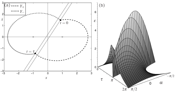
Figure 2: Panel (a): visualization of a colliding periodic orbit of (1), (2). Panel (b): collision surface in the three-dimensional parameter space $(\tau,\alpha,\varepsilon)$. Damping $\zeta$ is fixed at $-0.1$. At the parameters on the surface there exists a symmetric periodic orbit $L$ experiencing a corner collision. Beneath the surface the symmetric periodic orbit is a fixed point of the map $F_{+}$ in the subdomain $D_{+}$, above the surface it is a fixed point of the map $F_{-}$ in the subdomain $D_{-}$.

The affine flows $Y_{\pm}$ are given by

$$Y_{\pm}^{t}y=A(t)y\pm v(t)$$

where

$$\begin{split}A(t)&=e^{-\zeta t}\cos t-e^{-\zeta t}\sin t\begin{bmatrix}-\zeta&-1\\ 1+\zeta^{2}&\phantom{-}\zeta\end{bmatrix}\mbox{, and}\\ v(t)&=e^{-\zeta t}\begin{bmatrix}-\zeta\sin t-\cos t+e^{\zeta t}\\ (1+\zeta^{2})\sin t\end{bmatrix}\end{split}$$

and have equilibria at $(\pm 1,0)^{T}$. The condition for the existence of a colliding symmetric periodic orbit is

$$\begin{split}y_{1}\cos\alpha+y_{2}\sin\alpha&=\phantom{-}\varepsilon\mbox{\quad for $\tau>\pi$\ }\\ y_{1}\cos\alpha+y_{2}\sin\alpha&=-\varepsilon\mbox{\quad for $\tau<\pi$}\end{split}$$ (21)

where $y=-[I+A(\tau)]^{-1}v(\tau)$ (thus, $y=-Y_{+}^{\tau}y$). For $\zeta<0$, condition (21) ensures that the switching point $y$ lies on the switching manifold and that $f_{2}=f(y,1)$ points out of the hysteresis region. See Figure 2(a) for a visualization of a symmetric periodic orbit satisfying the collision condition (21). Figure 2(b) shows the surface of parameters $(\tau,\alpha,\varepsilon)$ where a colliding symmetric orbit $L$ exists in system (20). Whenever one varies the system parameters along a path intersecting the surface transversally $L$ undergoes a corner collision. Beneath the surface $L$ is a fixed point of $F_{+}$ in $D_{+}$, above the surface $L$ is a fixed point of $F_{-}$ in $D_{-}$.

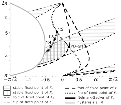
Figure 3: Bifurcations of the maps $F_{+}$ and $F_{-}$ projected onto the corner collision surface (‘look from above’ onto the surface in Figure 2(b)). Damping $\zeta$ is fixed at $-0.1$. Only the part of the collision surface with positive $\varepsilon$ is shown. Thick lines are standard bifurcations of $F_{-}$. Thin lines are standard bifurcations of $F_{+}$. The cross is a coincidence of a Neimark-Sacker bifurcation of $F_{-}$ with the corner collision at $\varepsilon=0.1$. Its numerical unfolding is presented in Figure 4 and Figure 6.

The change of stability of the fixed point of $F$ at the corner collision is determined by the linearizations of $F_{-}$ and $F_{+}$. Figure 3 shows a map of the different eigenvalue configurations that can occur on the collision parameter surface for $\tau\in(\pi,2\pi)$. The map $F_{+}$ has a one-dimensional image. Thus, the linearization of $F_{+}$ in its fixed point has only one non-zero eigenvalue. The horizontally hatched region in Figure 3 shows where this eigenvalue has modulus less than one. Within this region the fixed point of $F_{+}$ is stable at collision. Consequently, the symmetric periodic orbit of (20) is linearly stable for parameters beneath the horizontally hatched region in Figure 3 of the collision surface in Figure 2(b). The stable region of $F_{+}$ is bounded by a flip bifurcation (eigenvalue equals $-1$, thin dotted in Figure 3) and a fold bifurcation (or saddle-node, eigenvalue equals $1$, thin dashed in Figure 3). Parameter values on a bifurcation curve in Figure 3 correspond to codimension two events of the oscillator (20) because they also lie on the collision surface. This means that the symmetric periodic orbit of (20), as a fixed point of $F$, has a linearization with neutral stability in one of the subdomains $D_{\pm}$ and, simultaneously, it is located on the boundary between $D_{-}$ and $D_{+}$.

The map $F_{-}$ has a two-dimensional image. Thus, the linearization in its fixed point has two potentially non-zero eigenvalues. The vertically hatched region in Figure 3 shows parameter values where both eigenvalues are inside the unit circle. In this region above the collision surface the oscillator has a symmetric periodic orbit that is linearly stable as a fixed point of $F_{-}$. The standard bifurcations of the fixed point of $F_{-}$ are shown as thick lines (flip dotted, fold dashed, Neimark-Sacker hollow). Along the Neimark-Sacker bifurcation (also called torus bifurcation) curve a complex conjugate pair of eigenvalues is on the unit circle. All of the bifurcation curves of $F_{-}$ correspond to codimension two events for the symmetric periodic orbit of the oscillator (20) because they occur simultaneously with the collision, lying on the collision surface in the three-dimensional parameter space shown in Figure 2(b).

Remarks

The flip bifurcation of $F_{\pm}$ corresponds to a symmetry breaking bifurcation of the original symmetric periodic orbit of the oscillator (20) because the return map along the full periodic orbit is the second iterate of $F$.

The line $\alpha=0$ in the figures 2(b) and 3 corresponds to the case of pure position feedback studied in [7]. The linearizations of $F_{+}$ and $F_{-}$ coincide for $\alpha=0$. More precisely, the expressions for $g_{+}$ and $g_{-}$ in (19) are identical. It has been observed in [7] that non-smooth phenomena cannot occur for symmetric periodic orbits at the event collision.

The points $(\alpha,\tau)=(0,\pi)$ and $(\alpha,\tau)=(0,2\pi)$ in Figure 3 are highly degenerate. The periodic orbit does not intersect the switching line transversally at these parameter values, violating the strict transversality condition (13). The collision surface is singular for $\tau=\pi$.

Figure 3 shows codimension two degeneracies of the linearization of $F_{-}$ such as a concurrence of eigenvalues $-1$ and $+1$ at PD-SN and strong resonances along the Neimark-Sacker bifurcation (double eigenvalue $-1$ at 1:2, eigenvalues $\exp(\pm 2\pi i/3)$ at 1:3, eigenvalues $\pm i$ at 1:4, see [20] for an analysis and description). These points correspond to codimension three bifurcations of the symmetric periodic orbit. Similarly, all crossings of bifurcations of $F_{-}$ and bifurcations of $F_{+}$ in Figure 3 correspond to codimension three bifurcations of the symmetric periodic orbit. Other bifurcations of higher codimension that can occur along the bifurcation curves shown in Figure 3 involve the degeneracy of higher order terms in the normal form. These special points have been omitted from Figure 3.

The interaction PD-SN between the flip and the fold of the fixed point of the map $F_{-}$appears degenerate in Figure 3 in the following sense. The flip curve crosses the fold curve transversally instead of touching it quadratically as one would expect in a generic parameter unfolding [19]. This is due to the projection of the bifurcation curves onto the collision surface. The set of all parameters in the $(\tau,\alpha,\varepsilon)$-space where the fixed point of $F_{-}$ is a saddle-node forms a surface. This surface does not intersect the collision surface shown in Figure 2(b) transversally but touches it tangentially in the (dashed thick) fold bifurcation curves of Figure 3. The same applies to the fold of the fixed point of $F_{+}$.

6 Unfolding of Neimark-Sacker bifurcation collision

The symmetric periodic orbit $L$ of the oscillator (20) is stable near its corner collision in the hatched regions in Figure 3. Where the two hatched regions overlap $L$ is stable for parameters on both sides of the collision surface in Figure 2(b). Of primary interest are the parameter regions near bifurcation curves bounding the region of stability of $L$. In these regions we can expect that other (possibly stable) invariant objects exist near $L$, which in turn collide with the boundary $D_{0}$ between the two subdomains $D_{-}$ and $D_{+}$ of the phase space. In order to understand the dynamics near one of the codimension two events one has to unfold it using two parameters.

A systematic classification of possible unfoldings of codimension two bifurcations of piecewise smooth maps is not available in contrast to the situation for smooth systems [20]. Due to the impossibility of a general center manifold reduction it is difficult to derive general results. The references [2, 3, 9, 18] give a long list of possible cases but discuss unfoldings only for very few concrete examples.

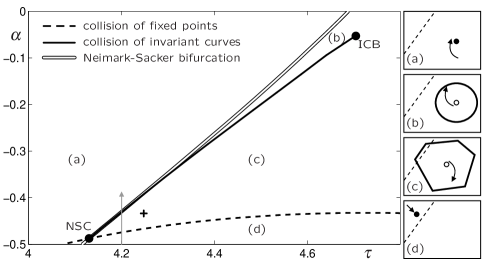
Figure 4: Unfolding of colliding Neimark-Sacker bifurcation in $(\tau,\alpha)$-plane. Values of other parameters: $\varepsilon=0.1$, $\zeta=-0.1$. All curves have been obtained by direct numerical continuation. The sketches on the right show qualitatively the dynamics in the different regions (a)–(d) (the dashed line is the switching line, attractors are solid, repellors hollow). Figure 5 shows the attracting invariant polygon at the parameter value marked by a cross. Figure 6 shows a parameter sweep of simulations along the gray arrow.

In this section we describe in detail the dynamics near the symmetric periodic orbit $L$ near a collision of a Neimark-Sacker bifurcation of $F_{-}$ with the boundary $D_{0}$. This case is only possible due to the increase of the dimension of the phase space from one (in $D_{+}$) to two (in $D_{-}$). In this sense it is the most characteristic feature of the symmetric corner collision of the oscillator (20). It is also the most complex case due to the involvement of invariant curves.

We fix $\varepsilon=0.1$. The plane $\{(\tau,\alpha,\varepsilon):\varepsilon=0.1\}$ intersects the collision surface of Figure 2(b) along a curve (not shown in Figure 3) and it intersects the Neimark-Sacker bifurcation on the collision surface (thick hollow curve) in a point NSC. This point NSC is marked by a cross in Figure 3 and corresponds to a set of parameters where the periodic orbit $L$ is on the boundary $D_{0}$, the linearization of $F_{-}$ has a complex conjugate pair of eigenvalues on the unit circle, and the linearization of $F_{+}$ is stable. We unfold this codimension two event using the parameter $\alpha$ (tilting angle of the switching line) and the delay $\tau$. Figure 4 shows the bifurcation diagram in the $(\tau,\alpha)$-plane. The point NSC corresponds to the cross mark in Figure 3. The dynamics in the different regions is sketched in the insets next to the diagram in Figure 4.

Let us explain the dynamics in the different regions near NSC (as sketched in the insets to the right of the diagram in Figure 4). In parameter region (a) $L$ is in region $D_{-}$. $L$ is a fixed point of $F_{-}$ and it is linearly stable, its linearization having a pair of complex conjugate eigenvalues inside the unit circle. On the Neimark-Sacker bifurcation curve (hollow) this pair of eigenvalues is exactly on the unit circle. Thus, $L$ changes its stability here. Moreover, the Neimark-Sacker bifurcation of $L$ does not have a strong resonance (see Figure 3 where the strong resonances are marked).

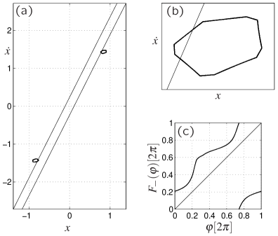
Figure 5: Attracting piecewise smooth invariant curve. Parameter values: $\alpha=-0.44$, $\tau=4.25$, $\varepsilon=0.1$, $\zeta=-0.1$ (cross in Figure 4). Panel (a) shows the switching points of the trajectory of the oscillator (20) in the $(x,\dot{x})$-plane. The switching lines are drawn as solid lines. Panel (b) zooms into the neighborhood of the attractor of $F$. Panel (c) shows the circle map on the closed polygon.

Consequently, a smooth closed invariant curve (invariant under $F_{-}$) emerges from $L$ at the Neimark-Sacker bifurcation near NSC. In this case the Neimark-Sacker bifurcation is supercritical, which implies that the emerging closed invariant curve is stable and exists in the region of linear instability of $L$ (region (b) in Figure 4). As the diameter of the invariant curve grows it collides with the boundary $D_{0}$. This collision occurs along the solid curve in Figure 4.

At this collision the smooth closed invariant curve disappears. In region (c) trajectories from all initial conditions close to $L$ (except $L$ itself) will eventually visit the region $D_{+}$. Thus, they will eventually follow the map $F_{+}$ at least once getting projected onto $\operatorname{rg}F_{+}$, a one-dimensional manifold. Since the fixed point of $F_{+}$ is stable and in region $D_{-}$ (thus, it is not a fixed point of $F$) all trajectories starting from points in $D_{+}$ will eventually visit $D_{-}$. Hence, in region (c) all trajectories map back and forth between the two regions $D_{-}$ and $D_{+}$.

This gives rise to invariant sets composed of finitely many smooth arcs that are images of a section of $\operatorname{rg}F_{+}$ under $F_{-}$. Since $F_{-}$ is approximately a rotation these arcs are rotations of $\operatorname{rg}F_{+}$. Their composition forms a piecewise smooth closed invariant curve consisting of finitely many arcs (a closed invariant polygon), which is located partially in $D_{-}$ and partially in $D_{+}$. This type of invariant set has been found and discussed for a piecewise linear map already in [30, 31], and for flows in [32, 33]. Figure 5 shows an example of such a polygon at the parameter values marked by a cross in Figure 4. Figure 5(a) shows the switching points of the trajectory of the original oscillator (20) (where the discrete component $u$ changes its value). Figure 5(b) is a zoom into the vicinity of the upper switching region, showing the attractor of $F$. Figure 5(c) shows the map restricted to the invariant polygon parametrized by the angle $\varphi$ of the point on the polygon relative to the the average of the attractor inside the curve. The map is clearly invertible giving rise to either quasi-periodicity or a pair of periodic orbits (locking) on the polygon. According to [31] non-invertible maps on polygons (and, hence, in principle chaotic dynamics) are also possible but we did not encounter this phenomenon close to NSC. See also [30, 31] for a study of resonance and locking phenomena on the invariant polygons.

If the parameters approach the collision curve of $L$ (dashed curve in Figure 4) the invariant polygons shrink as the fixed points of $F_{+}$ and $F_{-}$ approach each other (and the boundary $D_{0}$). Thus, in region (d) only the stable fixed point of $F_{-}$ in $D_{-}$ exists.

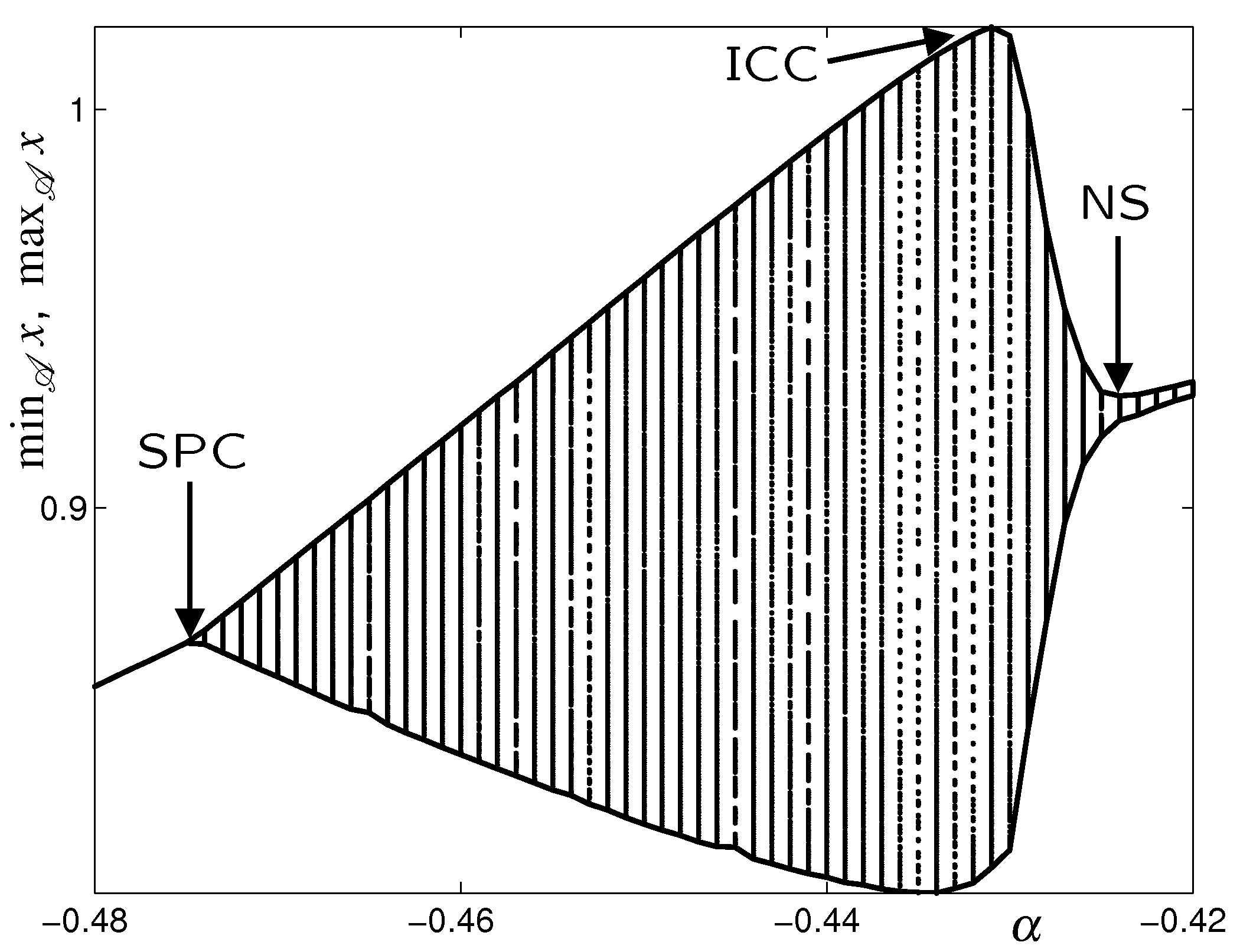
Figure 6: One-parameter pseudo bifurcation diagram for varying $\alpha$. Values of other parameters: $\tau=4.2$, $\varepsilon=0.1$, $\zeta=-0.1$ (along the gray arrow of Figure 4). Envelope contains maximum and minimum of the iterates of $F$ between $40$ and $400$ iterations. SPC, ICC and NS point out the intersection with the bifurcation curves in Figure 4.

Figure 6 shows the result of a parameter sweep along the gray arrow in Figure 4 showing the maximum and the minimum of the attractor ($\max F^{j}(y_{0})$ and $\min F^{j}(y_{0})$ for $j=40,\ldots,400$, restarting such that $y_{0}$ is the last iterate from the previous parameter). The figure gives evidence that the diameter of the invariant polygons grows linearly in the parameter $\alpha$, starting from the point SPC where the corner collision of $L$ occurs. During the sweep the polygon also changes its shape (for example, the number of corners or ‘overshoot’ of its edges). A detailed analysis how invariant polygons change under variation of the rotation and the linear expansion of the two-dimensional map $F_{-}$ is carried out in [32]. The polygon attracts in finite time between the points SPC and ICC in Figure 6 such that the numerical result shown in the plot is very accurate for this region. The detection of the collision of the smooth invariant curve near ICC, the family of smooth invariant curves and the Neimark-Sacker bifurcation NS are, however, only inaccurately accessible by pure simulations due to the weak attraction in region $D_{-}$.

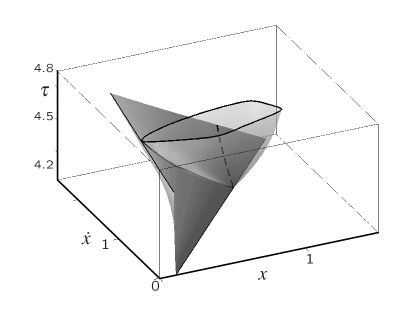
Figure 7: Family of closed invariant curves along collision curve (solid) in $(\tau,\alpha)$-plane of Figure 4, projected into the $(x,\dot{x},\tau)$-space. The value of $\alpha$ is coded by the gray value. Values of other parameters: $\varepsilon=0.1$, $\zeta=-0.1$. The family of invariant curves is the transparent cone. The dashed curve inside the cone are the unstable equilibria of $F$. The fanned out intransparent surface are the switching lines. The points where the invariant curves touch the switching lines are marked as a solid black curve lying on the cone and the intransparent surface.

Neimark-Sacker bifurcations and colliding smooth invariant curves can be efficiently computed directly because only the smooth two-dimensional map $F_{-}$ and the expression for the boundary $D_{0}$ are involved. The Neimark-Sacker bifurcation in Figure 4 can be accurately and efficiently continued using standard numerical algorithms as described in detail in [20] and implemented in AUTO [13]. The smooth closed invariant curve is given implicitly by the invariance equation

$$y(\eta(\varphi))=-Y_{+}^{\,\tau+t(\varphi)}y(\varphi)\mbox{,\quad}\varepsilon=[\cos\alpha,\sin\alpha]\cdot Y_{-}^{\,t(\varphi)}y(\varphi)$$ (22)

where $y(\varphi)$ is given by

$$y(\varphi)=y_{0}+r(\varphi)\begin{bmatrix}\cos\varphi\\ \sin\varphi\end{bmatrix}$$ (23)

and $y_{0}$ is the equilibrium of $F_{-}$:

$$y_{0}=-Y_{+}^{\,\tau+t_{0}}y_{0}\mbox{,\quad}\varepsilon=[\cos\alpha,\sin\alpha]\cdot Y_{-}^{\,t_{0}}y_{0}\mbox{.}$$ (24)

The equations (22)–(24) have the periodic functions $r(\varphi)$, $\eta(\varphi)$ and $t(\varphi)$, the vector $y_{0}\in\mathbb{R}^{2}$ and the scalar $t_{0}$ as variables. The definition of $y(\varphi)$ via (23) corresponds to a parametrization of the invariant curve by angle with respect to the equilibrium $y_{0}$. The function $r$ is the distance of the point on the invariant curve from $y_{0}$, $\eta$ is the circle map and $t$ is the time elapsed from the last switch (the map $F_{-}$ is defined only implicitly). This parametrization can be expected to work only in two-dimensional maps and for convex curves. Close to the point NSC in Figure 4 (in fact, close to the Neimark-Sacker curve) the invariant curves are ellipses and, thus, convex, making the parametrization (23) regular. We extend system (22)–(24) by the collision condition

$$0=\max_{\varphi\in(0,2\pi]}t(\varphi)\mbox{.}$$ (25)

The right-hand-side of (25) is a smooth function of $\varphi$ close to the point NSC in Figure 4 due to the convexity of the invariant curve. Thus, the system of equations (22)–(25) for the variables $(r,\eta,t,y_{0},t_{0},\tau,\alpha)$ defines a smooth family of colliding closed invariant curves which can be found by a Newton iteration with pseudo-arclength embedding [17]. Its projection into the $(\tau,\alpha)$-plane is shown as a solid curve in Figure 4. The closed invariant curves of the colliding family projected into the space $(x,\dot{x},\tau)$ are depicted (as a transparent gray cone) in Figure 7. Figure 7 gives evidence of the linear dependence of the radius $r$ of the closed invariant curve on the parameter $\tau$. Thus, the solid collision curve must be quadratically tangent to the Neimark-Sacker curve at NSC in Figure 4 because the radius $r$ has square root like asymptotics with respect to the distance of the parameter value to the Neimark-Sacker bifurcation. At the point ICB the invariant curve is close to a break-up such that the numerical approximation (32 complex Fourier modes) of $r$ and $\eta$ gives an error estimate greater than $10^{-2}$.

Remarks

If the Neimark-Sacker bifurcation is subcritical then the line of collisions of closed invariant curves (solid) lies on the other side of the Neimark-Sacker bifurcation (hollow) in Figure 4 (but still tangential). The polygons remain stable filling the region between the solid and the dashed curve.

The interaction between flip bifurcation and collision (dotted curves in Figure 3) has been analyzed in [18]. A periodic orbit $L_{2}$ of period two branches off from $L$. In any generic two-parameter unfolding a curve of collisions of $L_{2}$ emerges tangentially to the flip curve of $L$ (looking very similar to Figure 4, replacing the Neimark-Sacker curve by a flip curve and the collision of the invariant curve by a collision of $L_{2}$). The dynamics of the system between the collision of $L_{2}$ and the collision of the period-one orbit $L$ has, for example in [18], a stable period-two orbit flipping between the subdomains $D_{-}$ and $D_{+}$.

7 Conclusions and open problems

The local bifurcation theory of periodic orbits in hybrid dynamical systems with delayed switching can be reduced to the study of low-dimensional maps because the local return map (Poincaré map) of periodic orbits is finite-dimensional. The codimension one events for generic systems (corner collision and tangential grazing) were studied in [27]. This paper studies the case of simultaneous corner collision due to reflection symmetry, a case that has been encountered frequently in example studies [4, 5, 7, 15].

The presence of hysteresis in the switch simplifies the proof of the reduction theorem (Theorem 9), given here for the first time. However, the statement of the reduction theorem remains valid also without hysteresis.

The derivation of Theorem 9 can be generalized in a straightforward manner to other discrete symmetries and other than binary switches (with more notational overhead) as long as the symmetry can be reduced locally near the periodic orbit.

The reduction extends the applicability of theory and numerical methods that have been developed for smooth and piecewise smooth low-dimensional maps to systems with delayed switches. On the numerical side this includes direct continuation of periodic orbits and their bifurcations and discontinuity induced events (such as grazing and collision) and the continuation of smooth invariant curves. Robust and universal methods for continuation and detection of discontinuity induced bifurcations for periodic orbits have been developed by Piiroinen [24, 25]. Methods for the continuation of closed invariant curves have a longer history. Schilder [26] and Thakur [8] present recent implementations, the papers also give surveys of earlier work. There is, however, a large gap between recent developments of numerical methods for closed invariant curves and piecewise smooth systems and their actual availability in the form of software. Due to this gap the investigation of the oscillator in Section 6 could not rely on generally available tools.

The analysis of the oscillator shows that dynamical phenomena of hybrid systems with delayed switches can be systematically discovered with the help of numerical continuation and the reduction theorem. Two major open problems can be identified from the results of this analysis and the comparison to other results.

First, there is a gap between the relatively simple local bifurcation theory of periodic orbits as presented here and in [27] and the abundance and variety of complex phenomena observed in detailed example studies such as [4, 7, 15]. In particular, many of the complex phenomena (say, chaotic attractors that have periodic orbits with various switching patterns embedded) cannot be reached by systematic continuation of periodic orbits and branching off at continuous local bifurcations. One of the reasons behind this gap is the presence of discontinuous events such as the grazing and the corner collision with $q<0$ presented in Section 4.1. These events are beyond the scope of local bifurcation theory because some trajectories leave the local neighborhood of the periodic orbit. A way to close this gap may be the study of discontinuous events under the assumption of the existence of a smooth ‘global’ return map for trajectories leaving the neighborhood similar to the treatment of global bifurcations of smooth dynamical systems.

The second open question is the robustness of discontinuity induced bifurcations with respect to singular perturbations. For example, do the closed invariant polygons (as shown in Figure 5) persist when we change the oscillator (1) to

$$\ddot{x}+\zeta y+\omega^{2}x=u\mbox{,\quad}\beta\dot{y}=\dot{x}-y$$ (26)

(a modification to non-viscous damping for visco-elastic materials [1]) with a small $\beta$? In particular, are there still finitely many smooth arcs? Note that the argument of [31] and of Section 6 that the arcs are images under $F_{-}$ of the one-dimensional image $\operatorname{rg}F_{+}$ cannot be applied anymore because $\dim\,\operatorname{rg}F_{+}=2$ for (26). Most statements of the bifurcation theory for piecewise smooth systems cannot be easily generalized to higher dimensions due to the lack of center manifolds. For example, the limit of small delay $\tau$, which is governed by standard singular perturbation theory for smooth dynamical systems [6], is highly non-regular for (1) in the case of $\varepsilon=0$, see [27].

Appendix A Basic properties of the forward evolution

Let $\xi_{0}\in C([-\Theta,0];\mathbb{R}^{n})$ be the initial history segment of the continuous variable $y$ (where $\Theta\geq\tau$) and $u_{0}\in\{-1,1\}$ be the initial state of the discrete variable $u$ in system (4), (5). How does this initial state evolve to time $T$ (defining the evolution $E^{T}(\xi_{0},u_{0})$?

First, we define $E^{T}(\xi_{0},u_{0})$ for $T\in(0,\tau]$ using the variation of constants formulation of (4). We define the following subsets of the closed interval $[-\tau,0]$:

$$\begin{split}R_{+}&=\{s\in[-\tau,0]:h(\xi_{0}(s))\leq-\varepsilon\}\\ R_{-}&=\{s\in[-\tau,0]:h(\xi_{0}(s))\geq\varepsilon\}\\ R_{0\ }&=\{s\in[-\tau,0]:h(\xi_{0}(s))\in(-\varepsilon,\varepsilon)\}\mbox{.}\end{split}$$

The set $R_{0}$ is open relative to $[-\tau,0]$. Thus, if non-empty it is a union of countably many disjoint open (relative to $[-\tau,0]$) intervals. We arrange this sequence of countably many disjoint intervals into two subsequences of intervals: $I^{+}_{j}$ ($j=1,\ldots$), $I^{-}_{j}$ ($j=1,\ldots$) and, possibly, one extra interval $I_{0}$:

$$\begin{split}I^{+}_{j}&=\mbox{intervals of $R_{0}$ that have a lower boundary $s^{+}_{j}\in R_{+}$, i.e., $h(\xi_{0}(s^{+}_{j}))=-\varepsilon$,}\\ I^{-}_{j}&=\mbox{intervals of $R_{0}$ that have a lower boundary $s^{-}_{j}\in R_{-}$, i.e., $h(\xi_{0}(s^{-}_{j}))=\varepsilon$,}\\ I_{0}&=\begin{cases}[-\tau,t_{0})\quad\mbox{ \begin{minipage}[t]{303.53267pt} if $-\tau\in R_{0}$ (then $t_{0}$ is the upper boundary of the left-most interval of $R_{0}$) \end{minipage} }\\ \emptyset\quad\mbox{if $-\tau\notin R_{0}$.}\end{cases}\end{split}$$

We define the following function $\chi:[0,\tau]\mapsto\mathbb{R}$:

$$\chi(s)=\begin{cases}\phantom{-}1&\quad\mbox{if $s-\tau\in R_{+}\cup\bigcup_{j}I^{+}_{j}$}\\ -1&\quad\mbox{if $s-\tau\in R_{-}\cup\bigcup_{j}I^{-}_{j}$}\\ \phantom{-}u_{0}&\quad\mbox{if $s-\tau\in I_{0}$.}\end{cases}$$ (27)

Thus, $\chi$ is measurable on $[0,\tau]$ and either $1$ or $-1$ everywhere. The variation-of-constants formulation of (4) is

$$y(t)=\xi_{0}(0)+\int_{0}^{t}f(y(s),+1)\frac{[1+\chi(s)]}{2}+f(y(s),-1)\frac{[1-\chi(s)]}{2}\,ds.$$ (28)

This is a fixed point problem on the space $C([0,\tau];\mathbb{R}^{n})$ of continuous functions on the interval $[0,\tau]$ that has a globally unique solution $y(\cdot)\in C([0,\tau];\mathbb{R}^{n})$ due to the Lipschitz continuity of $f(\cdot,\pm 1)$. Then, for $T\in(0,\tau]$, $E^{T}(\xi_{0},u_{0})=(\xi(T)(\cdot),u(T))$ is defined by

$$\begin{split}\xi(T)(s)&=\begin{cases}y(T+s)&\quad\mbox{if $s\in[-T,0]$,}\\ y_{0}(T+s)&\quad\mbox{if $s\in[-\tau,-T]$,}\end{cases}\\ u(T)&=\chi(T)\mbox{.}\end{split}$$ (29)

We observe that the initial value of the discrete variable $u_{0}$ only affects the result $E^{T}(y_{0},u_{0})$ if $h(\xi_{0}(-\tau))\in(-\varepsilon,\varepsilon)$. Otherwise, (29) simply sets the discrete variable to its consistent value. For $T>\tau$ we define $E^{T}(\xi_{0},u_{0})$ as a concatenation of smaller time steps, for example, if $T\in[(k-1)\tau,k\tau]$ then $E^{T}=E^{T/k}\circ\ldots\circ E^{T/k}$. This definition is independent of the particular partition of $[0,T]$.

The definition of the evolution $E$ using the variation-of-constants formulation (28) allows one to initialize $E$ from arbitrary continuous history segments $\xi_{0}$ and discrete states $u_{0}$ even if $\xi_{0}$ crosses the switching manifolds $\{h(x)=\pm 1\}$ infinitely often or if $u_{0}$ is ‘inconsistent’. Due to (28) the continuous component $E_{c}$ of $E^{T}(y_{0},u_{0})$ depends continuously on $T$. If $T\geq\tau$ then $E_{c}^{t}(\xi_{0},u_{0})$ is Lipschitz continuous with respect to $t$. Its Lipschitz constant is $L_{\max}\cdot\|E_{c}^{t}(\xi_{0},u_{0})|_{t\in[t_{0},t_{E}]}\|$ where $L_{\max}$ is the Lipschitz constant of the right-hand-side $f$. For positive times the trajectory of the discrete component $E_{d}$ is continuous from the right, that is $\lim_{s\searrow t}E_{d}^{s}(\xi_{0},u_{0})=E_{d}^{t}(\xi_{0},u_{0})$ for all $t>0$.

Proof of Lemma 1

(Point 1)  Let $\delta>0$ be such that $|s-t|<\delta$ implies $|h(\xi_{0}(s))-h(\xi_{0}(t))|<2\varepsilon$ for all $s,t\in[-\tau,0]$. This $\delta$ exists because the initial value $\xi_{0}\in C([-\tau,0];\mathbb{R}^{n})$ is uniformly continuous and $h$ is Lipschitz continuous.

We have to check how many sign changes the function $\chi$, defined in (27), can have in the interval $[0,\tau]$. Let us denote the upper boundary of each interval $I^{\pm}_{j}$ by $t^{\pm}_{j}$. If $I_{0}$ is non-empty $\chi$ can change its sign only in $[t_{0},\tau]$ (one change is, possibly, in $t_{0}$). If $I_{0}$ is empty we will use the notation $t_{0}=0$ in the following argument.

After $t_{0}$ the function $\chi$ changes from $-1$ to $1$ only at times $t=t^{-}_{j}+\tau$ when $t^{-}_{j}\in R_{+}$, that is, $h(\xi_{0}(s^{-}_{j}))=\varepsilon$ (by definition of $I^{-}_{j}$) and $h(\xi_{0}(t^{-}_{j}))=-\varepsilon$. By definition of $\delta$ this implies that $t^{-}_{j}\geq s^{-}_{j}+\delta$. Hence, $\chi=-1$ for at least time $\delta$ before it can switch to $1$. The same argument applies for intervals $I^{+}_{j}$ and $\chi$ switching from $1$ to $-1$. Consequently, between two subsequent switchings of $\chi$ a time of at least $\delta$ must elapse. This limits the number of switchings to a finite number on a bounded interval.

Point 2: After time $\tau$ the constant $\delta$ in the above argument is bounded from below by

$$\delta\geq\frac{2\varepsilon}{H_{\max}L_{\max}\max\|y\|}$$ (30)

where $y$ is the solution of the fixed point problem for the variation-of-constants formulation (28), $H_{\max}$ is the Lipschitz constant of switching function $h$, and $L_{\max}$ is the Lipschitz of the right-hand-side $f$.

Proof of Lemma 4 (continuity)

It is sufficient to prove the continuity of $E_{c}^{T}(\xi,u)$ with respect to $\xi$ in $\xi_{*}=y_{*}(t+\cdot)\in C([-\Theta,0];\mathbb{R}^{n})$ and $u=u_{*}(t)$ for times $T\leq\tau$ because $(y_{*},u_{*})$ is periodic.

Due to the Lipschitz continuity of $f(\cdot,\pm 1)$ in the variation-of-constants formulation (28) it is sufficient to prove that, for any given $\Delta>0$, we can find a neighborhood $U(\xi_{*})$ such that

$$\int_{0}^{T}|E_{d}^{s}(\xi,u_{*}(t))-u_{*}(t+s)|\,ds<2\Delta$$ (31)

for all $\xi\in U(\xi_{*})$. That is, we have to show that, starting from $\xi$, we follow the same flow as $y_{*}$ all the time in $[0,T]$ except in a union of intervals of overall length $\Delta$. Let $t_{*,k}$ ($k=1,\ldots,\mu$) be the crossing times of $\xi_{*}$ in $[-\tau,0]$. Let us denote by $u_{k}$ the value of the discrete variable $u_{*}$ at time $t$ and at the switching times in $[t,t+\tau]$, that is, $u_{0}=u_{*}(t)$, $u_{k}=u_{*}(t+\tau+t_{*,k})$ ($k=1,\ldots,\mu$). Since $u_{*}$ is continuous from the right $u_{*}(t+\tau+s)=u_{k}$ also for $s$ slightly larger than $-\tau$ and $t_{*,k}$ ($k=1,\ldots,\mu$).

Due to the weak transversality of $(y_{*},u_{*})$ for all sufficiently small $\delta_{1}>0$ there exists a $\delta_{2}>0$ such that

1. $-\delta_{2}\geq u_{k}\cdot h(y_{*}(t+t_{*,k}+\delta_{1}))+\varepsilon$ for all $k=1,\ldots,\mu$, and

2. $-\delta_{2}\geq u_{k-1}h(y_{*}(t+s))-\varepsilon$ for all $s\in[t_{*,k-1},t_{*,k}-\delta_{1}]$ (for $k=2,\ldots,\mu$) and $s\in[-\tau,t_{*,1}-\delta_{1}]$.

Both statements follow from the strict monotonicity of $|h(y_{*}(\cdot)|$ at crossing times of $(y_{*},u_{*})$ and the identities $u_{k}h(y_{*}(t+t_{*,k}))+\varepsilon=0$ and $u_{k-1}h(y_{*}(t+t_{*,k}))-\varepsilon=0$. The points 1 and 2 imply that for all sufficiently small $\delta_{1}>0$ there exists an open neighborhood $U(\xi_{*})$ such that $\xi\in U(\xi_{*})$ satisfy

1. $0\geq u_{k}\cdot h(\xi(t_{*,k}+\delta_{1}))+\varepsilon$ for all $k=1,\ldots,\mu$, and

2. $0\geq u_{k-1}h(\xi(s))-\varepsilon$ for all $s\in[t_{*,k-1},t_{*,k}-\delta_{1}]$ (for $k=2,\ldots,\mu$) and $s\in[-\tau,t_{*,1}-\delta_{1}]$.

Consequently, for initial values $(\xi,u)$ with $\xi\in U(\xi_{*})$ and $u=u_{*}(t)$ the discrete variable $E_{d}^{s}(\xi,u)$ is equal to $u_{0}$ in $[0,\tau+t_{*,1}-\delta_{1}]$ and equal to $u_{k}$ in $[\tau+t_{*,k}+\delta_{1},\tau+t_{*,k+1}-\delta_{1}]$ for $k=1,\ldots,\mu-1$ and, if $t_{*,\mu}+\delta_{1}<0$, equal to $u_{\mu}$ in $[\tau+t_{*,\mu}+\delta_{1},\tau]$. Thus, $E_{d}^{s}(\xi,u)$ and $u_{*}(t+s)$ can be different only in $\mu+1$ intervals of length less than $2\delta_{1}$. Choosing $\delta_{1}=\Delta/(\mu+1)$ we obtain the neighborhood $U(\xi_{*})$ guaranteeing (31) for all $\xi\in U(\xi_{*})$.

Proof of Lemma 5

First we choose a $\delta>0$ sufficiently small such that $|h(y_{*}(s))|$ is strictly monotone increasing in all intervals $[t_{*,k}-\delta,t_{*,k}+\delta]$ where $t_{*,k}$ ($k=1,\ldots,\mu$) are the crossing times of the periodic orbit $(y_{*},u_{*})$ in $(-\tau,0)$. This $\delta$ exists due to the weak transversality of $(y_{*},u_{*})$. We define the constant

$$c_{0}=\min_{k=1,\ldots,\mu}\left\{|h(y(t_{*,k}-\delta))|-\varepsilon|,|h(y(t_{*,k}+\delta))|-\varepsilon|\right\}\mbox{,}$$

which is positive. Thus, $|h(y_{*}(t_{*,k}-\delta)|-\varepsilon\leq-c_{0}$ and $|h(y_{*}(t_{*,k}+\delta))|-\varepsilon\geq c_{0}$. We choose $U_{1}(\xi_{*})$ such that for all $\xi\in U_{1}(\xi_{*})$

$$\max_{k=1,\ldots,\mu}\left\{|h(\xi(t_{*,k}-\delta))-h(y_{*}(t_{*,k}-\delta))|,|h(\xi(t_{*,k}+\delta))-h(y(t_{*,k}+\delta))|\right\}\leq c_{0}/2\mbox{.}$$

This guarantees that $|h(\xi(\cdot))|-\varepsilon$ changes its sign in $[t_{*,k}-\delta,t_{*,k}+\delta]$ for all $\xi\in U(\xi_{*})$. Consequently, there exist unique times $t_{k}$ ($k=1,\ldots,\mu$) such that

$$t_{k}=\min\{t\in[t_{*,k}-\delta,t_{*,k}+\delta]:|h(\xi(t))|=\varepsilon\}\mbox{,\quad($k=1,\ldots,\mu$).}$$

If $\delta$ is sufficiently small $E_{d}^{t}(\xi,1)$ will change its value exactly at the times $t_{k}+\tau$ in $[0,\tau]$. This implies that $\xi^{\tau}=E_{c}^{\tau}(\xi,1)$ is given by the recursion (denoting $t_{0}=-\tau$ and $t_{\mu+1}=0$)

$$\begin{split}\xi^{\tau}(-\tau)&=\xi(0)\\ \xi^{\tau}(t)&=\begin{cases}Y_{-}^{[t-t_{k}]}\xi^{\tau}(t_{k})&\mbox{if $t\in(t_{k},t_{k+1}]$ and $k$ odd}\\ Y_{+}^{[t-t_{k}]}\xi^{\tau}(t_{k})&\mbox{if $t\in(t_{k},t_{k+1}]$ and $k$ even}\mbox{.}\end{cases}\end{split}$$

Hence, $\xi^{\tau}=E_{c}^{\tau}(\xi,1)$ depends only on $\xi(0)=y(0)$ and $t_{1},\ldots,t_{\mu}$. The discrete variable $E_{d}^{\tau}(\xi,1)$ equals $u_{*}(\tau)$. Therefore, $E^{p}(\xi,1)=E^{p-\tau}\circ E^{\tau}(\xi,1)$ also depends only on $\xi(0),t_{1},\ldots,t_{\mu}$.

Denote the continuous component $E_{c}^{p}(\xi,1)$ of $E^{p}(\xi,1)$ by $\xi^{p}$. The cross section $\Sigma$ is transversal to $y_{*}(\cdot)$ at $y_{*}(0)$. Thus, for every $y\in U(y_{*}(0))$ there exists a locally unique traveling time $t$ such that $Y_{+}^{t}y\in\Sigma$. The function $t_{\Sigma}:y\mapsto t$ is well defined (and smooth) in $U(y_{*}(0))$. If $U_{1}(\xi_{*})$ is sufficiently small then $\xi^{p}(0)\in U(y_{*}(0))$ due to the continuity of $E_{c}$ in $\xi_{*}=y_{*}(\cdot)$. The return time $T(\xi)$ is given by $T(\xi)=p+t_{\Sigma}(\xi^{p}(0))$. As $\xi^{p}$ depends only on $(\xi(0),t_{1},\ldots,t_{\mu})$ the same applies to $T(\xi)$ and, hence, the return map $P$.

Proof of Corollary 6

The condition 1 of Corollary 6 guarantees that the periodic orbit follows one of the flows in each of its crossing times $t_{*,k}\in(0,p)$ ($k=1,\ldots,m$), say, $Y_{k}$ ($Y_{k}=Y_{\pm}$). Condition 2 guarantees that the flow $Y_{k}$ intersects the switching manifold $\{|h|=\varepsilon\}$ transversally in $y_{*}(t_{*,k})$ for all crossing times $t_{*,k}$, that is, $h^{\prime}(y_{*}(t_{*,k}))\dot{Y}_{k}^{t}(y_{*}(t_{*,k}))|_{t=0}\neq 0$.

The coordinates $y_{0}\in\Sigma$ and $(t_{1},\ldots,t_{\mu})$ of an initial condition in $(\xi,1)\in{\cal S}_{1}$ must be in a small neighborhood of $(y_{*}(0),t_{*,m-\mu+1}-p,\ldots,t_{*,m}-p)$. Therefore, the headpoint $y(t)$ of $E_{c}^{t}(\xi,1)$ follows $Y_{k}$ at times near $t_{*,k}$ for $k=1,\ldots,m$ (because $y_{*}$ follows $Y_{k}$). Thus, the transversal intersection of $Y_{k}$ with the switching manifold near $t_{*,1},\ldots,t_{*,m}$ implies that the crossings of $y(t)$ near $t_{*,1},\ldots,t_{*,m}$ depend smoothly on the coordinates $(y_{0},t_{1},\ldots,t_{\mu})$. Consequently, also all times $t\in(0,p)$ when $E_{d}^{t}(\xi,1)$ changes its value depend smoothly on $(y_{0},t_{1},\ldots,t_{\mu})$. As the cross-section $\Sigma$ is transversal to $Y_{+}$ and $y(t)$ follows $Y_{+}$ for $t$ near $p$ the return time also depends smoothly on $(y_{0},t_{1},\ldots,t_{\mu})$ and, hence, the whole return map $P$ depends smoothly on the coordinates $y_{0}\in\Sigma$ and $(t_{1},\ldots,t_{\mu})$.

Appendix B Proof of Lemma 8 and Theorem 9

Proof of Lemma 8

The strict transversality condition (13) implies that the periodic orbit also satisfies the weak transversality condition (as given in Definition 3). In the proof of continuity (Lemma 4) we established that the discrete components $E_{d}^{t}(\xi,u)$ of trajectories starting from initial conditions $(\xi,u)$ near $(y_{*}(\cdot),u_{*}(0))$ change their values always close to times where $u_{*}$ changes its value. Also the direction of change must be the same because there is a minimum distance between subsequent changes (given in (30)). The colliding symmetric periodic orbit changes its value exactly twice per period, at $t=0$ and at $t=T$. Thus, the image $(\xi,u)$ of an initial value $(\xi_{0},u_{0})$ must have a continuous component $\xi$ switching exactly once near $s=-\Delta$ from $Y_{-}$ to $Y_{+}$. (The Poincaré section $\Sigma$ was taken at $y_{*}(\Delta)$ and $u_{*}$ switches from $-1$ to $1$ at $t=0$.)

Consequently, $\xi$ must have the form (14) for some $y\in U(y_{*}(0))$ and a time $\theta(y)$, which is the traveling time from $y$ to $\Sigma$ following $Y_{+}$. The only open question is if $\xi(0)\in\Sigma$ and the time $t_{1}(\xi)$ are uniquely determined by $y$.

Let $y\in U(y_{*}(0))$ be given. The time $\theta(y)$ is implicitly given by $Y_{+}^{\theta}y\in\Sigma$, which means

$$f_{2}^{T}[Y_{+}^{\theta}y-y_{*}(\Delta)]=0\mbox{.}$$ (32)

The linearization of (32) in $y=y_{*}(0)$ with respect to $\theta$ is $f_{2}^{T}f_{2}$, which is non-zero due to the strict transversality (13). Thus, $\theta$ is a locally unique and well defined function of $y$. Consequently, $\xi(0)=Y_{+}^{\theta}y$ is also well defined and smoothly dependent on $y$. The time $t_{1}=t_{1}(\xi)$ is given by $t_{1}=t(y)-\theta(y)$ where $t$ is implicitly defined by

$$\varepsilon = h(Y_{+}^{t}y)\mbox{\quad if $h(y)<\varepsilon$,}$$ (33)

$$\varepsilon = h(Y_{-}^{t}y)\mbox{\quad if $h(y)\geq\varepsilon$.}$$ (34)

The linearization with respect to $t$ in $y=y_{*}(0)$ is $h^{\prime T}f_{2}$ in case (33) and $h^{\prime T}f_{1}$ in case (34). Both linearizations are non-zero due to the strict transversality condition (13).

Proof of Theorem 9

Let $y\in U(y_{*}(0))$ be given. Lemma 8 gives a unique element $\xi$ of the image of $P$ corresponding to $y$ that has the form (14). The image of $y$ under the map $m$ is the location $y_{2}$ at the next time $s_{2}$ when the discrete component $E_{d}^{s_{2}}(\xi,1)$ changes its value from $-1$ to $+1$. The full reflection symmetry of the periodic orbit $L$ implies that $m$ is the second iterate of a map $F:U(y_{*}(0))\mapsto U(y_{*}(0))$ which is defined as $-y_{1}$ where $y_{1}$ is the location at the next time $s_{1}$ when the discrete component $E_{d}^{s_{1}}(\xi,1)$ changes its value from $+1$ to $-1$.

The regular implicit condition (32) defines $\theta(y)$ and $\xi(0)$. The regular implicit condition (16) (same as (33), (34)) defines the time $t_{1}(y)=t(y)-\theta(y)$ locally uniquely. Thus, the $E_{d}^{s}(\xi,1)$ changes its value to $-1$ at time $s_{1}=\tau+t_{1}(y)$. The point $y_{1}$ is the headpoint of the continuous component $E_{c}^{s_{1}}(\xi,1)$. It has the form

$$y_{1}=Y_{+}^{s_{1}}\xi(0)=Y_{+}^{s_{1}+\theta(y)}y=Y_{+}^{\tau+t(y)}y$$

because $t_{1}=t(y)-\theta(y)$ where $t(y)$ is given by the regular implicit condition (16). Thus, $F(y)=-y_{1}$ has the form claimed in Theorem 9.

References

- [1] S. Adhikari. Qualitative dynamic characteristics of a non-viscously damped oscillator. Proceedings of the Royal Society A: Mathematical, Physical and Engineering Sciences, 461(2059):2269–2288, 2005.
- [2] S. Banerjee and C. Grebogi. Border collision bifurcations in two-dimensional piecewise smooth maps. Phys. Rev. E, 59:4052–4061, 1999.
- [3] S. Banerjee, P. Ranjan, and C. Grebogi. Bifurcations in two-dimensional piecewise smooth maps – theory and applications in switching circuits. IEEE Transactions on Circuits and Systems – 1: Fundamental Theory and Applications, 47(5):633–643, 2000.
- [4] D.A.W. Barton, B. Krauskopf, and R.E. Wilson. Periodic solutions and their bifurcations in a non-smooth second-order delay differential equation. Dynamical Systems: An international Journal, 21(3):289–311, 2006.
- [5] W. Bayer and U. an der Heyden. Oscillation types and bifurcations of a nonlinear second-order differential-difference equation. J. Dynam. Diff. Eq., 10(2):303–326, 1998.
- [6] C. Chicone. Inertial and slow manifolds for delay equations with small delays. Journal of Differential Equations, 190:364–406, 2003.
- [7] A. Colombo, M. di Bernardo, S.J. Hogan, and P. Kowalczyk. Complex dynamics in a hysteretic relay feedback system with delay. J. Nonlinear Sci., 2006. online first, http://dx.doi.org/10.1007/s00332-005-0745-y.
- [8] H. Dankowicz and G. Thakur. A Newton method for locating invariant tori of maps. Internat. J. Bifur. Chaos Appl. Sci. Engrg., 16(5):1491–1503, 2006.
- [9] M. di Bernardo, C. Budd, A.R. Champneys, and P. Kowalczyk. Piecewise-smooth Dynamical Systems — Theory and Applications, volume 163 of Applied Mathematical Sciences. Springer-Verlag, 2007.
- [10] M. di Bernardo, M.I. Feigin, S.J. Hogan, and M.E. Homer. Local analysis of C-bifurcations in n-dimensional piecewise smooth dynamical systems. Chaos, Solitons and Fractals, 10:1881–1908, 1999.
- [11] M. di Bernardo, K.H. Johansson, and Francesco Vasca. Self-oscillations and sliding in relay feedback systems: symmetry and bifurcations. International Journal of Bifurcation and Chaos, 11(4):1121–1140, 2001.
- [12] Odo Diekmann, Stephan A. van Gils, Sjoerd M. Verduyn Lunel, and Hans-Otto Walther. Delay equations, volume 110 of Applied Mathematical Sciences. Springer-Verlag, New York, 1995. Functional, complex, and nonlinear analysis.
- [13] E. J. Doedel, A. R. Champneys, T. F. Fairgrieve, Y. A. Kuznetsov, B. Sandstede, and X. Wang. AUTO97, Continuation and bifurcation software for ordinary differential equations. Concordia University, 1998.
- [14] L. Fridman, E. Fridman, and E. Shustin. Steady modes and sliding modes in relay control systems with delay. In J. P. Barbot and W. Perruquetti, editors, Sliding Mode Control in Engineering, pages 263–293. Marcel Dekker, New York, 2002.
- [15] U. Holmberg. Relay feedback of simple systems. PhD thesis, Lund Institute of Technology, 1991.
- [16] K. H. Johansson, A Rantzer, and K. J. Astrom. Fast switches in relay feedback systems. Automatica, 35(4):539–552, 1999.
- [17] I. G. Kevrekidis, R. Aris, L. D. Schmidt, and S. Pelikan. Numerical computation of invariant circles of maps. Phys. D, 16(2):243–251, 1985.
- [18] P. Kowalczyk, M. di Bernardo, A.R. Champneys, S.J. Hogan, M. Homer, P.T. Piiroinen, Y.A. Kuznetsov, and A. Nordmark. Two-parameter discontinuity-induced bifurcations of limit cycles: classification and open problems. Internat. J. Bifur. Chaos Appl. Sci. Engrg., 16(3):601–629, 2006.
- [19] Y. A. Kuznetsov, H. G. E. Meijer, and L. van Veen. The fold-flip bifurcation. Internat. J. Bifur. Chaos Appl. Sci. Engrg., 14(7):2253–2282, 2004.
- [20] Yuri A. Kuznetsov. Elements of applied bifurcation theory, volume 112 of Applied Mathematical Sciences. Springer-Verlag, New York, third edition, 2004.
- [21] J. Lygeros, K.H. Johansson, S.N. Simić, J. Zhang, and S.S. Sastry. Dynamical properties of hybrid automata. IEEE Trans. on Automatic Control, 48(1):2–17, 2003.
- [22] U. F. Moreno, P. L. D. Peres, and I. S. Bonatti. Analysis of piecewise linear-oscillators with hysteresis. Circuits and Systems I: Fundamental Theory and Application IEEE Transactions, 50:1120 – 1124, 2003.
- [23] H. Nusse, E. Ott, and J. Yorke. Border collision bifurcations: an explanation for observed bifurcation phenomena. Phys. Rev. E, 49:1073––1076, 1994.
- [24] P. T. Piiroinen, L. N. Virgin, and A. R. Champneys. Chaos and period-adding: experimental and numerical verification of the grazing bifurcation. J. Nonlinear Sci., 14(4):383–404, 2004.
- [25] P.T. Piiroinen and Y.A. Kuznetsov. An event-driven method to simulate filippov systems with accurate computing of sliding motions. ACM Transactions on Mathematical Software, 2007.
- [26] F. Schilder, H.M. Osinga, and W. Vogt. Continuation of quasi-periodic invariant tori. SIAM Journal on Applied Dynamical Systems, 4(3):459–488, 2005.
- [27] J. Sieber. Dynamics of delayed relay systems. Nonlinearity, 19(11):2489–2527, 2006.
- [28] D.J.W. Simpson and J.D. Meiss. Neimark-Sacker bifurcations in planar piecewise-smooth continuous maps. preprint, University of Colorado at Boulder, 2007.
- [29] G. Stépán. Retarded Dynamical Systems: Stability and Characteristic Functions. Longman Scientific and Technical, Harlow, Essex, 1989.
- [30] I. Sushko and L. Gardini. Business Cycle Dynamics — Models and Tools, chapter Center Bifurcation for a Two-Dimensional Piecewise Linear Map. Springer-Verlag, 2006.
- [31] I. Sushko, T. Puu, and L. Gardini. The Hicksian floor-roof model for two regions linked by interregional trade. Chaos, Solitons and Fractals, 18:593–612, 2003.
- [32] R. Szalai and H.M. Osinga. Invariant polygons in systems with grazing-sliding. submitted, preprint available at http://hdl.handle.net/1983/948.
- [33] E. Zhusubaliyev, Z.T.; Mosekilde. Torus birth bifurcations in a DC/DC converter. Circuits and Systems I: Regular Papers, IEEE Transactions on [Circuits and Systems I: Fundamental Theory and Applications, IEEE Transactions on], 53(8):1839–1850, 2006.