Modeling the Non-Thermal X-ray Tail Emission of Anomalous X-ray Pulsars

Abstract

The paradigm for Anomalous X-ray Pulsars (AXPs) has evolved recently with the discovery by INTEGRAL and RXTE of flat, hard X-ray components in three AXPs. These non-thermal spectral components differ dramatically from the steeper quasi-power-law tails seen in the classic X-ray band in these sources, and can naturally be attributed to activity in the magnetosphere. Resonant, magnetic Compton upscattering is a candidate mechanism for generating this new component, since it is very efficient in the strong fields present near AXP surfaces. In this paper, results from an inner magnetospheric model for upscattering of surface thermal X-rays in AXPs are presented, using a kinetic equation formalism and employing a QED magnetic scattering cross section. Characteristically flat and strongly-polarized emission spectra are produced by non-thermal electrons injected in the emission region. Spectral results depend strongly on the observer’s orientation and the magnetospheric locale of the scattering, which couple directly to the angular distributions of photons sampled. Constraints imposed by the Comptel upper bounds for these AXPs are mentioned.

1 Introduction

A topical focus of the high energy astrophysics of compact objects over the last decade has been the so-called magnetars (Duncan & Thompson 1992), constituted by Soft-Gamma Repeaters (SGRs) and Anomalous X-ray Pulsars (AXPs), whose amassed observational properties have indicated that they are isolated neutron stars with ultra-strong magnetic fields. The AXPs, are a group of 6–7 pulsating X-ray sources with periods around 6-12 seconds. They are bright, possessing peak luminosities $\,L_{\hbox{\sevenrm X}}\sim 10^{35}\,\rm erg\;s^{-1}\,$, show no sign of any companion, are steadily spinning down and have ages $\,\tau\mathrel{\mathchoice{\lower 2.0pt\vbox{\halign{$\m@th\displaystyle\hfil#\hfil$\cr<\crcr\sim\crcr}}}{\lower 2.0pt\vbox{\halign{$\m@th\textstyle\hfil#\hfil$\cr<\crcr\sim\crcr}}}{\lower 2.0pt\vbox{\halign{$\m@th\scriptstyle\hfil#\hfil$\cr<\crcr\sim\crcr}}}{\lower 2.0pt\vbox{\halign{$\m@th\scriptscriptstyle\hfil#\hfil$\cr<\crcr\sim\crcr}}}}10^{5}\,$ years (e.g. Vasisht & Gotthelf 1997). Details of the persistent pulsed X-ray emission for AXPs are discussed in Tiengo et al. (2002), for XMM observations of 1E 1048.1-5937, and Juett et al. (2002) and Patel et al. (2003), for the Chandra spectrum of 4U 0142+61. This emission displays both thermal contributions, which have $\,kT\sim 0.5-1\,$ keV and so are generally hotter than those in isolated pulsars, and also non-thermal components with steep spectra that can be fit by power-laws $\,dn/dE\propto E^{-s}\,$ of index in the range $\,s=2-3.5\,$ (see Perna et al., 2001, for spectral fitting of ASCA data on AXPs).

The recent detection by the IBIS imager on INTEGRAL, and the PCA and HEXTE detectors of the Rossi X-ray Timing Explorer, of hard, non-thermal pulsed tails in three AXPs has provided a new twist to the AXP phenomenon. In all of these, the differential spectra above 20 keV are extremely flat: 1E 1841-045 (Kuiper, Hermsen & Mendez 2004) has a power-law energy index of $\,s=0.94\,$ between around 20 keV and 150 keV, 4U 0142+61 displays an index of $\,s=0.2\,$ in the 20 keV – 50 keV band, with a steepening at higher energies implied by the total DC+pulsed spectrum (Kuiper et al. 2006), and RXS J1708-4009 has $\,s=0.88\,$ between 20 keV and 150 keV (Kuiper et al. 2006). The tails are much flatter than the non-thermal spectra in the $\,<10\,$ keV band, and do not continue much beyond the IBIS energy window: there are strongly constraining upper bounds from Comptel observations of these sources that necessitate a break somewhere in the 150–750 keV band (see Figures 4, 7 and 10 of Kuiper et al. 2006).

This paper summarizes results from our initial exploration (Baring & Harding 2007) of the production of non-thermal X-rays by inverse Compton heating of soft, atmospheric thermal photons by relativistic electrons, serving as a model for generating the hard X-ray tails in AXPs. The electrons are presumed to be accelerated along either open or closed field lines with super-Goldreich-Julian densities, perhaps by electrodynamic potentials, or large scale currents associated with twists in the magnetic field structure (e.g. Thompson & Beloborodov 2005). In the strong fields of the inner magnetospheres of AXPs, the inverse Compton scattering is predominantly resonant at the cyclotron frequency, with an effective cross section well above the classical Thomson value. Hence, proximate to the neutron star surface, in regions bathed intensely by the surface soft X-rays, this process is extremely efficient for an array of magnetic colatitudes, probably dominating other processes such as synchrotron and bremsstrahlung radiation that are employed in the models of Thompson & Beloborodov (2005) and Heyl & Hernquist (2005). This prospect motivates the investigation of resonant inverse Compton models. Here, the general character of emission spectra is presented, using collision integral analyses that will set the scene for future explorations using Monte Carlo simulations.

2 Resonant Compton Upscattering in AXPs

In devising any radiation emission model to describe the non-thermal X-ray tail luminosity from AXPs, it is necessary to ascertain the criteria that must be satisfied in order to explain the energetics. These were discussed in Baring & Harding (2007), who determined that for radiative processes that were electromagnetic in origin, i.e. involved electrons, the requisite electron densities must be super-Goldreich-Julian. This requirement is rather general in nature, not being constrained to just the resonant Compton upscattering scenario that is the focus here, but being coupled to a presence of relativistic electrons moving along B, with an abundance that can power the intense AXP X-ray luminosities, $\,L_{\hbox{\sevenrm X}}\mathrel{\mathchoice{\lower 2.0pt\vbox{\halign{$\m@th\displaystyle\hfil#\hfil$\cr>\crcr\sim\crcr}}}{\lower 2.0pt\vbox{\halign{$\m@th\textstyle\hfil#\hfil$\cr>\crcr\sim\crcr}}}{\lower 2.0pt\vbox{\halign{$\m@th\scriptstyle\hfil#\hfil$\cr>\crcr\sim\crcr}}}{\lower 2.0pt\vbox{\halign{$\m@th\scriptscriptstyle\hfil#\hfil$\cr>\crcr\sim\crcr}}}}10^{35}\,$erg/sec above 10 keV (Kuiper et al. 2006). The hard X-ray tail luminosities are 2–3 orders of magnitude greater than the classical spin-down luminosity $\,{\dot{E}}_{\hbox{\fiverm SD}}\sim 8\pi^{4}B_{p}^{2}R^{6}/(3P^{4}c^{3})\,$ due to magnetic dipole radiation torques, where $\,B_{p}\,$ is the surface polar field strength, $\,P\,$ is the pulsar period and $\,R\,$ is the stellar radius.

Here we briefly recapitulate the energetics analysis of Baring & Harding (2007). Let $\,n_{e}\,$ be the number density of emitting electrons, $\,\langle\gamma_{e}\rangle\,$ be their mean Lorentz factor, and $\,\epsilon_{\hbox{\sevenrm rad}}\,$ be the radiative efficiency during their traversal of the magnetosphere, either along open or closed field lines. Then $\,L_{\hbox{\sevenrm X}}\sim\epsilon_{\hbox{\sevenrm rad}}\langle\gamma_{e}\rangle m_{e}c^{2}(4\pi n_{e}R_{c}^{2}c)\,$ if the emission column has a base that is a spherical cap of radius $\,R_{c}<R\,$. If $\,R_{c}\sim 10^{6}\,$cm, this yields number densities $\,n_{e}\sim 3\times 10^{17}L_{\hbox{\sevenrm X,35}}/\epsilon_{\hbox{\sevenrm rad}}\langle\gamma_{e}\rangle\,$ cm^-3 for scaled luminosities $\,L_{\hbox{\sevenrm X,35}}\equiv L_{\hbox{\sevenrm X}}/10^{35}\,$erg/sec. Comparing $\,en_{e}\,$ to the classic Goldreich-Julian (1969) density $\,\rho_{\hbox{\fiverm GJ}}=\nabla.\vec{E}/4\pi=-\vec{\Omega}.\vec{B}/(2\pi c)\,$ for force-free, magnetohydrodynamic rotators, one can establish the ratio

$$\hbox{${{\displaystyle en_{e}\vphantom{(}}\over{\displaystyle|\rho_{\hbox{\fiverm GJ}}|\vphantom{(}}}$}\;\approx\;\hbox{${{\displaystyle 4,670\vphantom{(}}\over{\displaystyle\epsilon_{\hbox{\sevenrm rad}}\langle\gamma_{e}\rangle\vphantom{(}}}$}\;\hbox{${{\displaystyle L_{X,35}\,P\vphantom{(}}\over{\displaystyle B_{15}R_{6}^{2}\vphantom{(}}}$}\quad,$$ (1)

for AXP pulse periods $\,P\,$ in units of seconds, polar magnetic fields $\,B_{15}\,$ in units of $\,10^{15}\,$Gauss, and cap radii $\,R_{6}\,$ in units of $\,10^{6}\,$cm. For $\,\epsilon_{\hbox{\sevenrm rad}}\langle\gamma_{e}\rangle\mathrel{\mathchoice{\lower 2.0pt\vbox{\halign{$\m@th\displaystyle\hfil#\hfil$\cr>\crcr\sim\crcr}}}{\lower 2.0pt\vbox{\halign{$\m@th\textstyle\hfil#\hfil$\cr>\crcr\sim\crcr}}}{\lower 2.0pt\vbox{\halign{$\m@th\scriptstyle\hfil#\hfil$\cr>\crcr\sim\crcr}}}{\lower 2.0pt\vbox{\halign{$\m@th\scriptscriptstyle\hfil#\hfil$\cr>\crcr\sim\crcr}}}}10^{3}\,$ and $\,R_{6}\sim 1\,$, the requisite density $\,n_{e}\,$ is super-Goldreich-Julian, but not dramatically so. No choice of radiation mechanism has been invoked in this line of reasoning. Yet observe that electron Lorentz factors of $\,\gamma_{e}\gg 10^{2}-10^{3}\,$ and their efficient resonant Compton cooling (i.e. $\,\epsilon_{\hbox{\sevenrm rad}}\sim 0.01-1\,$) are readily attained in isolated pulsars with $\,B\sim 0.1\,$ (e.g. see Sturner 1995; Harding & Muslimov 1998; Dyks & Rudak 2000). Such efficiencies should persist into the magnetar regime. To substantiate this assertion, observe that in the Thomson cooling regime, the resonant Compton cooling rate $\,|\dot{\gamma}_{e}|\sim(n_{s}\hbox{$\sigma_{\hbox{\fiverm T}}$}c)\,3\pi B^{2}/(4\alpha_{\hbox{\sevenrm f}}\gamma_{e}\varepsilon_{s}^{2})\,$ can be obtained from Eq. (17) of Baring & Harding (2007), correcting a missing factor of $\,\alpha_{\hbox{\sevenrm f}}=e^{2}/(\hbar c)\,$ in the denominator. The lengthscale $\,\lambda_{\hbox{\eightrm res}}=c/|\dot{\gamma}_{e}|\,$ for resonant cooling can then be estimated from the Planck spectrum photon number density $\,n_{s}\sim{\cal T}^{3}/\lambda_{\hbox{\sevenrm C}}^{3}\,$ at the surface, where the scaled temperature $\,{\cal T}=kT/(m_{e}c^{2})\,$ sets $\,\varepsilon_{s}\sim 3{\cal T}\,$, and $\,\lambda_{\hbox{\sevenrm C}}=\hbar/m_{e}c\,$ is the electron Compton wavelength over $\,2\pi\,$. The result is $\,\lambda_{\hbox{\eightrm res}}\sim(\lambda_{\hbox{\sevenrm C}}/\alpha_{\hbox{\sevenrm f}})\,\gamma_{e}/({\cal T}B^{2})\,$, lengthens considerably at high altitudes due to dilution of the soft photon density. For $\,B\sim 0.1\,$, $\,\gamma_{e}\sim 10^{3}\,$ and $\,{\cal T}\sim 3\times 10^{-3}\,$, $\,\lambda_{\hbox{\eightrm res}}\,$ is much less than the stellar radius, a result that is clearly not modified by relativistic quantum corrections when $\,B\mathrel{\mathchoice{\lower 2.0pt\vbox{\halign{$\m@th\displaystyle\hfil#\hfil$\cr>\crcr\sim\crcr}}}{\lower 2.0pt\vbox{\halign{$\m@th\textstyle\hfil#\hfil$\cr>\crcr\sim\crcr}}}{\lower 2.0pt\vbox{\halign{$\m@th\scriptstyle\hfil#\hfil$\cr>\crcr\sim\crcr}}}{\lower 2.0pt\vbox{\halign{$\m@th\scriptscriptstyle\hfil#\hfil$\cr>\crcr\sim\crcr}}}}1\,$.

By necessity, the locales where Compton interactions sample the cyclotron resonance are confined to the lower altitudes in an AXP magnetosphere, where the field is sufficiently high. This is controlled primarily by the scattering kinematics, which dictates a coupling between the energies $\,\varepsilon_{\gamma}m_{e}c^{2}\,$ and $\,\gamma_{e}m_{e}c^{2}\,$ of colliding X-ray photons and electrons, respectively, and the local angle $\,\theta_{\gamma}\,$ of the interacting photon to the magnetic field lines. The cyclotron fundamental is sampled when

$$\gamma_{e}\varepsilon_{\gamma}(1-\cos\theta_{\gamma})\;\approx\;B\quad,\quad\hbox{for}\;\gamma_{e}\;\gg\;1\quad.$$ (2)

For X-ray photons emanating from a single point on the stellar surface, Baring & Harding (2007) computed the zones of influence of the resonant Compton process for dipole field geometry in a flat spacetime. Assuming that the X-rays propagate with no azimuthal component to their momenta, the resonance criterion is satisfied on a surface that is azimuthally symmetric about the magnetic field axis, for slow rotators. For outward-going electrons, the locus of the projection of this surface onto a plane intersecting the magnetic axis was found to be

$$\chi^{3}\;=\;\Psi\;\hbox{${{\displaystyle\sqrt{1+3\cos^{2}\theta}\vphantom{(}}\over{\displaystyle 1-\cos\theta_{\gamma}\vphantom{(}}}$}\quad,\quad\Psi\;=\;\hbox{${{\displaystyle B_{p}\vphantom{(}}\over{\displaystyle 2\gamma_{e}\varepsilon_{\gamma}\vphantom{(}}}$}\quad,$$ (3)

where $\,\chi=r/R\,$ is the altitude scaled in units of the neutron star radius $\,R\,$, and $\,\theta\,$ is the magnetic colatitude of the point of scattering. $\,B_{p}\,$ is the surface polar field strength in units of $\,B_{\rm cr}=4.413\times 10^{13}\,$Gauss. Geometry determines the function, $\,\theta_{\gamma}=\theta_{\gamma}(\theta_{e},\,\theta)\,$, which is given in Eq. (5) of Baring & Harding (2007), where $\,\theta_{e}\,$ is the colatitude of the surface emission point. Here $\,\Psi\,$ is the key parameter that scales the altitude of the locale of resonant interaction, and typically falls in the range $\,1-10^{3}\,$ for magnetars when $\,\gamma_{e}\sim 10^{2}-10^{4}\,$. For the broadly representative cases of soft photons emitted from the surface pole ($\,\theta_{e}=0\,$) and magnetic equator ($\,\theta_{e}=90^{\circ}\,$), the surfaces of resonant scattering for different $\,\Psi\,$ are illustrated in Fig. 1. Shadows of the emission points are also indicated to mark propagation exclusion zones for the chosen emission colatitudes.

   

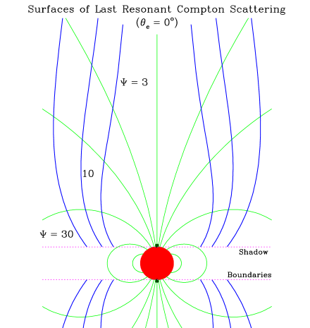
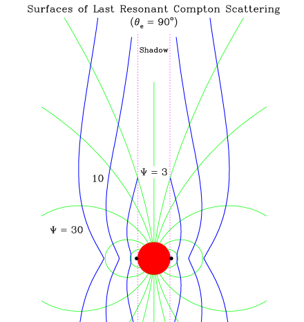
Figure 1: Contours in a section of a pulsar magnetosphere that depict cross sections of the surfaces of last resonant scattering by ultra-relativistic electons, i.e. the maximal extent of the Compton resonasphere. The heavyweight blue contours are computed for different values of the resonance parameter $\,\Psi\,$ defined in Eq. (3), and at extremely high altitudes asymptotically approach the magnetic axis (central vertical line). The filled red circles denote the neutron star, whose radius $\,R\,$ establishes the linear spatial scale for the Figure. The cases illustrated are for photons emanating from the polar axis (i.e. $\,\theta_{e}=0^{\circ}\,$, left panel) and from the equator (i.e. $\,\theta_{e}=90^{\circ}\,$ right panel), denoted by the small black dots, for which the neutron star shadow regions are demarcated by the light dotted boundaries, and only the surfaces (azimuthally-symmetric about the magnetic axis) are accessible to resonant Compton interactions.

It is evident from the Figure that the altitude of resonance is much lower for equatorial emission cases (comparing left and right panels), and also in the equatorial regions when compared with polar locales (within each panel). At small colatitudes above the magnetic pole, $\,\theta_{\gamma}\,$ is necessarily small, pushing the resonant surface to very high altitudes where the field is much lower. In equatorial interaction locales, which are preferentially sampled for quasi-equatorial emission colatitudes, the photons tend to travel more across field lines in the observer’s frame, and so access the resonance in regions of higher field strength, thereby reducing the altitudes where the resonance is sampled. These are manifestations of the correlation between $\,\theta_{\gamma}\,$ and $\,B\,$ (for fixed $\,\varepsilon_{\gamma}\,$ and $\,\gamma_{e}\,$) evinced in Eq. (2). For cases $\,0<\theta_{e}<90^{\circ}\,$ (not depicted), the contours are morphologically similar, though they incur significant deviations from those in Fig. 1. Clearly, by sampling different emission colatitudes $\,\theta_{e}\,$ these surfaces are smeared out into annular volumes. Observe that introducing an azimuthal component to the photon momentum tends to increase propagation across the field, i.e. raising $\,\theta_{\gamma}\,$, so that the resonance is accessed at lower altitudes and higher field locales. Hence, loci like those depicted in Fig. 1 actually represent the outermost extent of resonant interaction, and so are surfaces of last resonant scattering, i.e. the outer boundaries to the Compton resonasphere. It is evident that, for the majority of closed field lines for long period AXPs, this resonasphere is confined to within a few stellar radii of the surface.

2.1 Resonant Compton Upscattering Spectra

Collision integral calculations for upscattering spectra from resonant Compton interactions are routinely obtained for uniform magnetic fields. In the AXP problem, the scalelength $\,\lambda_{\hbox{\eightrm res}}\,$ for the interaction is often much shorter than the scale $\,R\,$ of the field divergence/gradient, so such uniform B computations are reasonably informative. Let $\,n_{\gamma}\,$ be the number density of photons resulting from the resonant upscattering process. For inverse Compton scattering, an expression for the spectrum of photon production $\,dn_{\gamma}/(dt\,d\varepsilon_{f}\,d\mu_{f})\,$, differential in the photon’s post-scattering laboratory frame quantities $\,\varepsilon_{f}\,$ and $\,\mu_{f}=\cos\Theta_{f}\,$, was presented in Eqs. (A7)–(A9) of Ho and Epstein (1989), valid for general scattering scenarios. The dimensionless pre- and post-scattering photon energies (i.e. scaled by $\,m_{e}c^{2}\,$) in the observer’s frame (OF) are $\,\varepsilon_{i}\,$ and $\,\varepsilon_{f}\,$, respectively, and the corresponding angles of these photons with respect to the OF electron velocity vector $\,-\vec{\beta}_{e}\,$ (i.e. field direction) are $\,\Theta_{i}\,$ and $\,\Theta_{f}\,$, respectively. The result for the spectrum can be integrated over $\,\mu_{f}\,$ and then written as (detailed in Baring & Harding, 2007)

$$\hbox{${{\displaystyle dn_{\gamma}\vphantom{(}}\over{\displaystyle dt\,d\varepsilon_{f}\vphantom{(}}}$}\,=\,\hbox{${{\displaystyle n_{e}n_{s}\,c\vphantom{(}}\over{\displaystyle\mu_{+}-\mu_{-}\vphantom{(}}}$}\int_{-1}^{1}d\mu_{f}\int_{\mu_{-}}^{\mu_{+}}d\mu_{i}\;\delta\big{[}\omega_{f}-\omega^{\prime}(\omega_{i},\,\theta_{f})\,\bigl{]}\,\hbox{${{\displaystyle 1+\beta_{e}\mu_{i}\vphantom{(}}\over{\displaystyle\gamma_{e}(1+\beta_{e}\mu_{f})\vphantom{(}}}$}\,\hbox{${{\displaystyle d\sigma\vphantom{(}}\over{\displaystyle d(\cos\theta_{f})\vphantom{(}}}$}\;\;.$$ (4)

Here, the notation $\,\mu_{i}=\cos\Theta_{i}\,$ and $\,\mu_{f}=\cos\Theta_{f}\,$ is used for compactness, $\,n_{e}\,$ and $\,n_{s}\,$ are the number densities of relativistic electrons and soft photons, respectively. For simplicity, the incident photons are assumed to be monoenergetic and to possess a uniform distribution of angle cosines $\,\mu_{i}\,$ in some range $\,\mu_{-}\leq\mu_{i}\leq\mu_{+}\,$. Note also that since $\,\gamma_{e}\gg 1\,$, the incident photon angle with respect to B in the electron rest frame (ERF) is $\,\theta_{i}\approx 0\,$, while the ERF angle $\,\theta_{f}\,$ of the scattered photon relative to the field can take on a range of values. The function $\,\omega^{\prime}(\omega_{i},\,\theta_{f})\,$, which appears in the $\,\delta\,$ function in Eq. (4), encapsulates the electron rest frame scattering kinematics, as detailed in Baring & Harding (2007). The differential cross section, $\,d\sigma/d(\cos\theta_{f})\,$, appearing in Eq. (4) is evaluated in the ERF, and is taken from Eq. (23) of Gonthier et al. (2000); it incorporates relativistic QED physics that is applicable for arbitrary field strengths. Specialized to the case of scatterings that leave the electron in the ground state, the zeroth Landau level that it originates from, its specific form is summarized in Baring & Harding (2007). More general results for the fully relativistic, quantum cross section for resonant Compton scattering can be found in Herold (1979), Daugherty & Harding (1986), and Bussard, Alexander & Mészáros (1986). These extend earlier non-relativistic quantum mechanical formulations such as in Canuto, Lodenquai & Ruderman (1971), and Blandford & Scharlemann (1976).

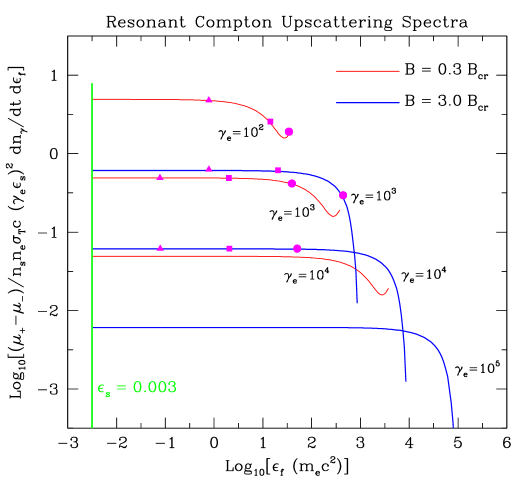
Figure 2: Resonant Compton upscattering spectra (scaled, unpolarized) such as might be sampled in the magnetosphere of an AXP, for different relativistic electron Lorentz factors $\,\gamma_{e}\,$, as labelled. The emergent photon energy $\,\varepsilon_{f}\,$ is scaled in terms of $\,m_{e}c^{2}\,$. The chosen magnetic field strengths of $\,B=3B_{\rm cr}\,$ (heavyweight, blue) and $\,B=0.3B_{\rm cr}\,$ (lighter weight, red) correspond to different altitudes and perhaps colatitudes. Results are depicted for seed photons of energy $\,\varepsilon_{s}=0.003\,$ (marked by the green vertical line), typical of thermal X-rays emanating from AXP surfaces; downscattering resonant emission at $\,\varepsilon_{f}<\varepsilon_{s}\,$ was not exhibited. Specific emergent angles of the emission in the observer’s frame, with respect to the magnetic field direction, are indicated by the filled magenta symbols for four of the spectra, with triangles denoting $\,\Theta_{f}=5^{\circ}\,$, squares corresponding to $\,\Theta_{f}=1^{\circ}\,$, and circles representing $\,\Theta_{f}=0.2^{\circ}\,$.

The relativistic Compton cross section $\,\sigma\,$ is strongly peaked at the cyclotron fundamental (see Fig. 2 of Gonthier et al. 2000) due to the appearance of resonant denominators in the S-matrices. These generate a Lorentz profile factor $\,1/[(\omega_{i}-B)^{2}+(\Gamma/2)^{2}]\,$ in $\,d\sigma/d(\cos\theta_{f})\,$, where $\,\Gamma=\Gamma_{\hbox{\sevenrm cyc}}\,E_{1}\,$ and $\,E_{1}=\sqrt{1+2B+\omega_{i}^{2}}\,$ is the energy of the intermediate electron. Here $\,\Gamma_{\hbox{\sevenrm cyc}}\ll B\,$ is the dimensionless cyclotron decay rate from the first Landau level (with electron momentum $\,p_{z}=\omega_{i}\,$ parallel to B), signifying that the intermediate electron states become effectively real at the cyclotron resonance, and possess a finite decay lifetime. A form for the decay rate $\,\Gamma_{\hbox{\sevenrm cyc}}\,$, can be found in Eqs. (13) or (23) of Baring, Gonthier & Harding (2005; see also Latal 1986; Harding & Lai 2006). For $\,B\ll 1\,$, $\,\Gamma_{\hbox{\sevenrm cyc}}\approx 4\alpha_{\hbox{\sevenrm f}}B^{2}/3\,$, while for $\,B\gg 1\,$, quantum and recoil effects generate $\,\Gamma_{\hbox{\sevenrm cyc}}\approx(\alpha_{\hbox{\sevenrm f}}/e)\sqrt{B/2}\,$. Note that Baring & Harding (2007) adopted the ansatz $\,\Gamma\to\Gamma_{\hbox{\sevenrm cyc}}\,$ appropriate for resonant Thomson scattering; here this is updated to incorporate relativistic corrections to the resonance width following Harding & Daugherty (1991), amounting to a spectral normalization correction by a factor of $\,1/\sqrt{1+2B}\,$ for all $\,\varepsilon_{f}\,$.

Representative spectral forms are depicted in Fig. 2, for the situation where emergent polarizations are not observed (see Baring & Harding 2007, for polarization characteristics). Because of the narrowness of the resonance, non-resonant scattering contributions were omitted when generating the curves; these contributions produce steep wings to the spectra at the uppermost and lowermost energies, and a slight bolstering of the flat portion. Generally they contribute significantly only when access to the resonance is kinematically forbidden, i.e. outside the Compton resonaspheres illustrated in Fig. 1. The resonant restriction kinematically limits the emergent photon energies $\,\varepsilon_{f}\,$ to

$$\gamma_{e}(1-\beta_{e})\,B\;\leq\;\varepsilon_{f}\;\leq\;\hbox{${{\displaystyle\gamma_{e}(1+\beta_{e})\,B\vphantom{(}}\over{\displaystyle 1+2B\vphantom{(}}}$}\quad,$$ (5)

a range that generally extends below the thermal photon seed energy $\,\varepsilon_{s}\,$. For the $\,B=0.3\,$ case in Fig. 2, a quasi-Thomson regime, the spectra are characteristically flat (e.g. see Dermer 1990; Baring 1994; Liu et al. 2006) for most $\,\varepsilon_{f}\,$, indicative of the kinematic sampling of the resonance in the integrations over soft photon angles $\,\Theta_{i}\,$. Since $\,\Gamma\ll B\,$ in general, the normalization of this flat portion scales as $\,dn_{\gamma}/(dt\,d\varepsilon_{f})\propto 1/\Gamma\,$. Only at the highest energies does the spectrum begin to deviate from flat (i.e. horizontal) behavior, and this domain corresponds to significant scattering angles in the ERF, i.e. cosines $\,1-\cos\theta_{f}\,$ not much less than unity. Then the mathematical form of the differential cross section becomes influential in determining the spectral shape, as discussed in Baring & Harding (2007). In AXPs, the $\,B=0.3\,$ case best represents higher altitude locales for the resonasphere, such as at smaller colatitudes near the polar axis. Fig. 2 also exhibits spectra for $\,B=3\,$, a case more typical of equatorial resonance locales. Then the flat spectrum still appears at energies $\,\varepsilon_{s}\leq\varepsilon_{f}\ll\gamma_{e}(1+\beta_{e})\,B/(1+2B)\,$, when again $\,\cos\theta_{f}\approx 1\,$. Yet the $\,B=3\,$ curves in the Figure display more prominent reductions at the uppermost energies $\,\varepsilon_{f}\sim\gamma_{e}(1+\beta_{e})\,B/(1+2B)\,$ due to the sampling of $\,1/2\leq\omega_{f}\ll\omega_{i}\,$ values in the ERF that correspond to strong electron recoil effects.

Photons emitted in these uppermost energies have $\,1-\cos\theta_{f}\sim 1\,$ in the ERF and are highly beamed along the field in the observer’s frame. This is an important property that is highlighted via the filled symbols in Fig. 2. The intense beaming of radiation along B in the OF, and the profound correlation of the angle of emission $\,\Theta_{f}\,$ with the emergent photon energy $\,\varepsilon_{f}\,$, are both consequences of scattering kinematics in the resonance. In the resonant case here, the $\,\gamma_{e}\gg 1\,$ regime dictates that most of the emission is collimated to within $\,5^{\circ}\,$ of the field direction, and rapidly becomes beamed to within $\,0.2^{\circ}\,$ as the final photon energy increases towards its maximum. This kinematic characteristic guarantees that spectral formation in Compton upscattering models is extremely sensitive to the observer’s viewing orientation in relation to the magnetospheric geometry. This suggests powerful geometrical probes of AXP emission regions if pulse-phase spectroscopy is achievable in future generation observatories.

3 Conclusion

This paper has summarized some essentials of the resonant Compton upscattering model for hard X-ray tail emission in AXPs, as developed in Baring & Harding (2007). The spectra exhibited in Fig. 2 are considerably flatter than the hard X-ray tails ($\,\sim\varepsilon_{f}^{-\alpha}\,$ for $\,\alpha\sim 0.2-1\,$) seen in the AXPs, and extend to GLAST-band energies much higher than can be permitted (i.e. around 750 keV) by the Comptel upper bounds to these sources, unless emergent angles $\,\Theta_{f}\,$ to B exceed around $\,1^{\circ}\,$. They represent a preliminary indication of how flat the resonant scattering process can render the spectrum, which can readily be steepened by spatial distribution of electron injection, significant and unavoidable cooling, and also non-resonant contributions. What an observer detects will depend critically on his/her viewing perspective and the magnetospheric locale of the scattering. The one-to-one kinematic coupling between $\,\varepsilon_{f}\,$ and $\,\mu_{f}\,$ implies that the highest energy photons are beamed strongly along the local field direction. This may or may not be sampled by an instantaneous observation at a given rotational phase. Realistically, for many pulse phases, angles corresponding to $\,\mu_{f}<1\,$ will be predominant, lowering the value of $\,\varepsilon_{f}\,$. How low is presently unclear, and remains to be explored via a model with full magnetospheric geometry, the obvious next development in this research program.

References

- (1)
- (2) Baring, M. G. 1994, in Gamma-Ray Bursts, eds. Fishman, G., Hurley, K. & Brainerd, J. J., (AIP Conf. Proc. 307, New York) p. 572.
- (3) Baring, M. G., Gonthier, P. L., Harding A. K. 2005, ApJ, 630, 430.
- (4) Baring, M. G. & Harding, A. K. 2007, Astr. Space Sci., 308, 109.
- (5) Blandford, R. D. & Scharlemann, E. T. 1976, MNRAS 174, 59.
- (6) Bussard, R. W., Alexander, S. B. & Mészáros, P 1986, Phys. Rev. D, 34, 440.
- (7) Canuto, V., Lodenquai, J. & Ruderman, M., 1971, Phys. Rev. D, 3, 2303.
- (8) Daugherty, J. K., & Harding, A. K. 1986, ApJ, 309, 362.
- (9) Dermer, C. D. 1990, ApJ, 360, 197.
- (10) Duncan, R. C. & Thompson, C. 1992, ApJ, 392, L9.
- (11) Dyks, J. & B. Rudak 2000, Astron. Astrophys. 360, 263.
- (12) Goldreich, P. & Julian, W. H. 1969, ApJ, 157, 869.
- (13) Gonthier, P. L., Harding A. K., Baring, M. G., Costello, R. M. & Mercer, C. L. 2000, ApJ, 540, 907.
- (14) Harding, A. K. & Daugherty, J. K., 1991, ApJ, 374, 687.
- (15) Harding, A. K. & Lai, D. 2006, Rep. Prog. Phys., 69, 2631.
- (16) Harding, A. K. & A. G. Muslimov 1998, ApJ, 508, 328.
- (17) Herold, H. 1979, Phys. Rev. D, 19, 2868.
- (18) Heyl, J. & Hernquist, L. E. 2005, MNRAS, 362, 777.
- (19) Ho, C, & Epstein, R. I. 1989, ApJ, 343, 227.
- (20) Juett, A. M., Marshall, H. L., Chakrabarty, D., et al. 2002, ApJ, 568, L31.
- (21) Kuiper, L., Hermsen, W., den Hartog, P. R., et al. 2006, ApJ, 645, 556.
- (22) Kuiper, L., Hermsen, W. & Mendeź, M. 2004, ApJ, 613, 1173.
- (23) Latal, H. G. 1986, ApJ, 309, 372.
- (24) Liu, D. B., Chen, L., You, J. H. & Zhang, S. N. 2006, MNRAS, 370, 911.
- (25) Patel, S. K., Kouveliotou, C., Woods, P. M., et al. 2003, ApJ, 587, 367.
- (26) Perna, R., Heyl, J. S., Hernquist, L. E., et al. 2001, ApJ, 557, 18.
- (27) Sturner, S. J. 1995, ApJ 446, 292.
- (28) Thompson, C. & Beloborodov, A. M. 2005, ApJ, 634, 565.
- (29) Tiengo, A., et al. 2002, A&A, 383, 182.
- (30) Vasisht, G. & Gotthelf, E. V. 1997, ApJ, 486, L129.