Joint Beamforming for Multiaccess MIMO Systems with Finite Rate Feedback^∗

Abstract

This paper considers multiaccess multiple-input multiple-output (MIMO) systems with finite rate feedback. The goal is to understand how to efficiently employ the given finite feedback resource to maximize the sum rate by characterizing the performance analytically. Towards this, we propose a joint quantization and feedback strategy: the base station selects the strongest users, jointly quantizes their strongest eigen-channel vectors and broadcasts a common feedback to all the users. This joint strategy is different from an individual strategy, in which quantization and feedback are performed across users independently, and it improves upon the individual strategy in the same way that vector quantization improves upon scalar quantization. In our proposed strategy, the effect of user selection is analyzed by extreme order statistics, while the effect of joint quantization is quantified by what we term “the composite Grassmann manifold”. The achievable sum rate is then estimated by random matrix theory. Due to its simple implementation and solid performance analysis, the proposed scheme provides a benchmark for multiaccess MIMO systems with finite rate feedback.

I Introduction

This paper considers multiaccess systems, corresponding to the uplink of cellular systems, where both the base station and the multiple users are equipped with multiple antennas. Multiple antenna systems, also known as multiple-input multiple-output (MIMO) systems, provide significant benefit over single antenna systems in terms of increased spectral efficiency and/or reliability. The full potential of MIMO though requires perfect channel state information (CSI) at both the transmitter and the receiver. While it is often reasonable to assume that the receiver has perfect CSI through a pilot signal, assuming perfect CSI at the transmitter (CSIT) is typically unrealistic. In many practical systems, the transmitter obtains CSI through a finite rate feedback from the receiver. Note that a wireless fading channel may have infinitely many channel states, and a finite rate feedback implies that CSIT is imperfect. One expects a performance degradation, and here we focus on the quantitative effect of finite rate feedback and the corresponding design.

Insight from single user MIMO systems with finite rate feedback proves beneficial. Single user systems are similar to multiaccess systems in the sense that there is only one receiver in both systems. The receiver knows the channel states perfectly and helps transmitters adapt their signals to maximize throughput. The essential difference between these two types of systems lies in the modes of antenna cooperation. In single user MIMO systems, all the transmit antennas are able to cooperate in sending a given message. In multiaccess systems, different users have independent messages, and transmit antennas belonging to one user cannot aid the transmission of another user’s message. Due to this additional constraint, the analysis and design of multiaccess systems becomes more complicated. Still, we will borrow insight from single user systems to simplify the design of multiaccess systems. For single user MIMO systems, strategies to maximize throughput with perfect CSIT and without CSIT are derived and analyzed in [1]. When only finite rate feedback is available, the focus has moved toward the development of suboptimal strategies as a simplification. The dominant approach is based on power on/off strategy, in which a data stream is either turned on with a pre-determined constant power or turned off (zero power). Systems with only one stream are considered in [2, 3, 4]. Systems with multiple independent streams are investigated in [5, 6, 7, 8, 9, 10, 11]. It appears that power on/off strategy is near optimal compared to the optimal power water-filling allocation [10].

We aim to understand how to efficiently employ the given finite feedback resource to maximize the sum rate by characterizing performance analytically. The full multiaccess MIMO problem still appears behind reach mathematically and is left for the future. In this paper, we propose a suboptimal strategy by borrowing insight and methods from single user systems. Specifically, the base station selects the strongest users, jointly quantizes their strongest eigen-channel vectors and broadcasts a common feedback to all the users. Instead of designing a specific quantization code book, we show that the performance of a random code book is optimal in probability. After receiving feedback information, a selected on-user employ power on/off strategy and transmit along the beamforming vector selected by the feedback. Here, joint quantization and feedback are employed based on the plain fact that vector quantization is better than scalar quantization [12, Ch. 13]. (The precise gain will be verified empirically.) It is also worth noting that, as we shall discuss in Section IV and V, antenna selection can be viewed as a simplified version of the proposed scheme.

This approach differs from the ongoing research for broadcast channels (BC) with finite rate feedback. While there is a well known duality between broadcast and multiaccess systems [13], this duality requires full CSI at both the transmitters and the receivers and is not available when only partial CSIT is provided. When CSIT is available only through finite rate feedback, broadcast systems suffer from the so called interference domination phenomenon [14, 15]. The major effort in research is to limit the interference among users. Sharif and Hassibi select the near orthogonal channels when the number of users is sufficiently large [14, 15]. As the number of users is comparable to the number of antennas at the base station, Jindal shows that the feedback rate should be proportional to signal-to-noise ratio (SNR) if the number of users turned on is fixed [15], while we show that the number of users should be adapt to the SNR if the feedback rate is given [16]. However, the interference domination phenomenon does not appear in multiaccess systems. Note that the search of near orthogonal channels suffers from exponential increasing complexity. Neither the results nor the methods for broadcast systems can be directly applied to the problem discussed in this paper.

Though the strategy in this paper is relatively simple, the corresponding performance analysis is nontrivial. Our main analytical result is an upper bound on the sum rate, which to our knowledge is the best to date. The effect of user/antenna selection is analyzed by extreme order statistics, and the effect of eigen-channel vectors joint quantization is quantified via the composite Grassmann manifold. Interestingly, the complicated effect of imperfect CSIT and feedback is eventually described by a single constant, which we term the power efficiency factor. Successful evaluation of the power efficiency factor enables us characterize the upper bound on the sum rate. The anticipated goodness of the upper bound is supported by simulation of several systems with a large range of SNRs.

The rest of this paper is organized as follows. The general model for multiaccess systems with finite rate feedback is described in Section II. The mathematical results developed for performance analysis are assembled in Section III. The antenna selection strategy is analyzed in Section IV-A. Then a suboptimal strategy is proposed and analyzed in Section IV-B. In Section V, simulation results are presented and discussed. Finally, Section VI summarizes the paper.

II System Model

Assume that there are $L_{R}$ antennas at the base station and $N$ users communicating with the base station. Assume that the user $i$ has $L_{T,i}$ transmit antennas $1\leq i\leq N$. Throughout we will set $L_{T,1}=\cdots=L_{T,N}=L_{T}$. The signal transmission model is

$$\mathbf{Y}=\sum_{i=1}^{N}\mathbf{H}_{i}\mathbf{T}_{i}+\mathbf{W},$$

where $\mathbf{Y}\in\mathbb{C}^{L_{R}\times 1}$ is the received signal at the base station, $\mathbf{H}_{i}\in\mathbb{C}^{L_{R}\times L_{T}}$ is the channel state matrix for user $i$, $\mathbf{T}_{i}\in\mathbb{C}^{L_{T}\times 1}$ is the transmitted Gaussian signal vector for user $i$ and $\mathbf{W}\in\mathbb{C}^{L_{R}\times 1}$ is the additive Gaussian noise vector with zero mean and covariance matrix $\mathbf{I}_{L_{R}}$. We assume the Rayleigh fading channel model: the entries of $\mathbf{H}_{i}$’s are independent and identically distributed (i.i.d.) circularly symmetric complex Gaussian variables with zero mean and unit variance ($\mathcal{CN}\left(0,1\right)$), and $\mathbf{H}_{i}$’s are independent across $i$.

We further assume that there exists a feedback link from the base station to the users. At the beginning of each channel use, the channel states $\mathbf{H}_{i}$’s are perfectly estimated at the receiver (the base station). This assumption is valid in practice since most communication standards allow the receiver to learn the channel states from pilot signals. A common message, which is a function of the channel states, is sent back to all users through the feedback link. We assume that the feedback link is rate limited and error-free. The feedback directs the users to choose their Gaussian signal covariance matrices. In a multiaccess communication system, different users cannot cooperate in terms of information message, leading to $\mathrm{E}\left[\mathbf{T}_{i}\mathbf{T}_{j}^{\dagger}\right]=\mathbf{0}$ for $i\neq j$. Let $\mathbf{T}=\left[\mathbf{T}_{1}^{\dagger}\cdots\mathbf{T}_{N}^{\dagger}\right]^{\dagger}$ be the overall transmitted Gaussian signal for all users and $\mathbf{\Sigma}\triangleq\mathrm{E}\left[\mathbf{T}\mathbf{T}^{\dagger}\right]$ be the overall signal covariance matrix. Then $\mathbf{\Sigma}$ is an $NL_{T}\times NL_{T}$ block diagonal matrix whose $i^{\mathrm{th}}$ diagonal block is the $L_{T}\times L_{T}$ covariance matrix $\mathrm{E}\left[\mathbf{T}_{i}\mathbf{T}_{i}^{\dagger}\right]$. Let $\mathbf{H}=\left[\mathbf{H}_{1}\mathbf{H}_{2}\cdots\mathbf{H}_{N}\right]$ be the overall channel state matrix. An extension of [17] shows that the optimal feedback strategy is to feedback the index of an appropriate covariance matrix, which is a function of current channel state $\mathbf{H}$. Last, assume that there is a covariance matrix codebook $\mathcal{B}_{\mathbf{\Sigma}}=\left\{\mathbf{\Sigma}_{1},\cdots,\mathbf{\Sigma}_{K_{\mathcal{B}}}\right\}$ (with finite size) declared to both the base station and the users, where each $\mathbf{\Sigma}_{k}\in\mathcal{B}_{\mathbf{\Sigma}}$ is the overall signal covariance matrix with block diagonal structure just described, and $K_{\mathcal{B}}$ is the size of the codebook. The feedback function $\varphi$ is a map from $\left\{\mathbf{H}\in\mathbb{C}^{L_{R}\times NL_{T}}\right\}$ onto the index set $\left\{1,\cdots,K_{\mathcal{B}}\right\}$. Subjected to this finite rate feedback constraint

$$\left|\mathcal{B}_{\mathbf{\Sigma}}\right|=K_{\mathcal{B}}$$

and the average total transmission power constraint

$$\mathrm{E}_{\mathbf{H}}\left[\mathrm{tr}\left(\mathbf{\Sigma}_{\varphi\left(\mathbf{H}\right)}\right)\right]\leq\rho,$$

the sum rate of the optimal feedback strategy is given by

$$\underset{\mathcal{B}_{\mathbf{\Sigma}}}{\sup}\;\underset{\varphi\left(\cdot\right)}{\sup}\;\mathrm{E}_{\mathbf{H}}\left[\log\left|\mathbf{I}_{L_{R}}+\mathbf{H}\mathbf{\Sigma}_{\varphi\left(\mathbf{H}\right)}\mathbf{H}^{\dagger}\right|\right].$$ (1)

Here, since only symmetric systems are concerned, the total power constraint $\rho$ is equivalent to individual power constraint $\rho/N$. Note that the optimal strategy involves two coupled optimization problems. It is difficult, if not impossible, to find its explicit form and performance. Instead, we shall study two suboptimal strategies and characterize their sum rates in Section IV.

III Preliminaries

This section assembles mathematical results required for later analysis. The reader may proceed directly to Section IV for the main engineering results.

III-A Order Statistics for Chi-Square Random Variables

Define $X_{i}=\sum_{j=1}^{L}\left|h_{i,j}\right|^{2}$ where $h_{i,j}\;1\leq j\leq L,\;1\leq i\leq n$ are i.i.d. $\mathcal{CN}\left(0,1\right)$. Then each $X_{i}$ has a Chi-square distribution with probability density functions (PDF)

$$f_{X}\left(x\right)=\frac{1}{\left(L-1\right)!}x^{L-1}e^{-x}.$$

Denote the corresponding cumulative distribution function (CDF) by $F_{X}\left(x\right)$. Next introduce the order statistics for these variables: that is the non-decreasing list $X_{\left(1:n\right)}\leq X_{\left(2:n\right)}\leq\cdots\leq X_{\left(n:n\right)}$ connected with each realization. Here, the subscript $\left(k:n\right)$ indicates that $X_{\left(k:n\right)}$ is the $k^{\mathrm{th}}$ minima. (We follow the convention of [18].) Note of course that ties occur with probability zero and can be broken arbitrarily.

We will need the following, which is proved in Appendix -B.

Lemma 1

With the notation set out above, for any fixed positive integer $s$ it holds

$$\underset{n\rightarrow+\infty}{\lim}\;\mathrm{E}\left[\frac{\sum_{k=1}^{s}X_{\left(n-k+1:n\right)}-sa_{n}}{b_{n}}\right]=s\left(\mu_{1}+1-\sum_{k=1}^{s}\frac{1}{k}\right),$$ (2)

where

$$a_{n}=\inf\left\{x:\;1-F_{X}\left(x\right)\leq\frac{1}{n}\right\},$$

$$b_{n}=\frac{\sum_{i=0}^{L-1}\frac{L-i}{i!}a_{n}^{i}}{\sum_{i=0}^{L-1}\frac{1}{i!}a_{n}^{i}},$$

and $\mu_{1}=\int_{-\infty}^{+\infty}xde^{-e^{-x}}$ may be computed numerically.

The limiting result in expectation immediately provides the following approximation for a fixed $s$:

$$\mathrm{E}\left[\sum_{k=1}^{s}X_{\left(n-k+1:n\right)}-sa_{n}\right]=sb_{n}\left(\mu_{1}+1-\sum_{i=1}^{s}\frac{1}{i}\right)\left(1+o\left(1\right)\right).$$ (3)

The shape of $F_{X}$ guarantees that $a_{n}$ and so $b_{n}$ are finite for any fixed $n$ but tend to infinity and one respectively with this parameter.

III-B Conditioned Eigenvalues of the Wishart Matrix

Let $\mathbf{H}\in\mathbb{L}^{n\times m}$ be a random $n\times m$ matrix whose entries are i.i.d. Gaussian random variables with zero mean and unit variance, where $\mathbb{L}$ is either $\mathbb{R}$ or $\mathbb{C}$. Throughout, we refer to $\mathbf{H}$ as the standard Gaussian random matrix. Let $\lambda_{1}\geq\lambda_{2}\geq\cdots\geq\lambda_{n}$ be the ordered eigenvalues of $\mathbf{W}=\mathbf{H}\mathbf{H}^{\dagger}$ ($\mathbf{W}$ is Wishart distributed [19]).

This subsection takes up an estimate of $\mathrm{E}\left[\left.\lambda_{1}\right|\mathrm{tr}\left(\mathbf{W}\right)\right]$, where $\mathrm{tr}\left(\cdot\right)$ is the usual matrix trace. In particular, while a closed formula for this object would be rather involved, we may use random matrix theory to obtain an approximation. The first ingredient is the following.

Lemma 2

Let $\mathbf{H}\in\mathbb{L}^{n\times m}$ (w.l.o.g. $n\leq m$) be a standard random Gaussian matrix. Let $\lambda_{1}\geq\lambda_{2}\geq\cdots\geq\lambda_{n}$ be the ordered eigenvalues of $\mathbf{W}=\mathbf{H}\mathbf{H}^{\dagger}$. Then

$$\mathrm{E}\left[\lambda_{i}|\mathrm{tr}\left(\mathbf{W}\right)=c\right]=\zeta_{i}c,$$

where

$$\zeta_{i}=\mathrm{E}\left[\lambda_{i}|\mathrm{tr}\left(\mathbf{W}\right)=1\right].$$ (4)

, (5)

$\beta=1$ if $\mathbb{L}=\mathbb{R}$ or $\beta=2$ if $\mathbb{L}=\mathbb{C}$, and $\left|\Delta_{n}\left(\bm{\lambda}\right)\right|=\prod_{i<j}^{n}\left(\lambda_{i}-\lambda_{j}\right)$.

Proof:

The joint density of the ordered eigenvalues of $\mathbf{W}$ is known to be

$$K_{m,n,\beta}^{-1}e^{-\frac{\beta}{2}\sum_{i}\lambda_{i}}\prod_{i=1}^{m}\lambda_{i}^{\frac{\beta}{2}\left(n-m+1\right)-1}\left|\Delta_{n}\left(\bm{\lambda}\right)\right|^{\beta},$$

where $\lambda_{1}\geq\cdots\geq\lambda_{m}\geq 0$, $\left|\Delta_{n}\left(\bm{\lambda}\right)\right|=\prod_{i<j}^{n}\left(\lambda_{i}-\lambda_{j}\right)$,

$$\beta=\begin{cases}1&\mathrm{if}\;\mathbb{L}=\mathbb{R}\\ 2&\mathrm{if}\;\mathbb{L}=\mathbb{C}\end{cases},$$

and $K_{m,n,\beta}$ is a normalizing factor ([19, pg. 107] for the real case and [1] for the complex case). Write out the formula for $\mathrm{E}\left[\lambda_{i}|\sum_{i=1}^{m}\lambda_{i}=c\right]$ and use the variable change $\lambda_{i}^{\prime}=\frac{\lambda_{i}}{c}$. After some elementary calculations, it can be shown that

$$\zeta_{i}=\frac{\int_{\underset{\lambda_{1}\geq\cdots\geq\lambda_{n}}{\sum\lambda_{j}=1}}\lambda_{i}\prod_{j=1}^{n}\lambda_{j}^{\frac{\beta}{2}\left(m-n+1\right)-1}\left|\Delta_{n}\left(\bm{\lambda}\right)\right|^{\beta}\prod_{j=1}^{n}d\lambda_{j}}{\int_{\underset{\lambda_{1}\geq\cdots\geq\lambda_{n}}{\sum\lambda_{j}=1}}\prod_{j=1}^{n}\lambda_{j}^{\frac{\beta}{2}\left(m-n+1\right)-1}\left|\Delta_{n}\left(\bm{\lambda}\right)\right|^{\beta}\prod_{j=1}^{n}d\lambda_{j}}=\mathrm{E}\left[\lambda_{i}|\mathrm{tr}\left(\mathbf{W}\right)=1\right].$$

∎

Given the preceding observation, we require an estimate for $\zeta_{1}$ in (5). For this we turn to the asymptotic behavior of the ordered eigenvalues.

Lemma 3

Let $\lambda_{1}\geq\lambda_{2}\geq\cdots\geq\lambda_{n}$ be the ordered eigenvalues of $\frac{1}{m}\mathbf{H}\mathbf{H}^{\dagger}$, where $\mathbf{H}\in\mathbb{L}^{n\times m}$ $\left(\mathbb{L}=\mathbb{R}\;\mathrm{or}\;\mathbb{C}\right)$ is a standard random Gaussian matrix. As $n,m\rightarrow\infty$ with $\frac{m}{n}\rightarrow\bar{m}\in\mathbb{R}^{+}$, for a given $\tau\in\left(0,\min\left(1,\bar{m}\right)\right)$,

$$\bar{\zeta}_{\tau} :=\underset{\left(n,m\right)\rightarrow\infty}{\lim}\mathrm{E}\left[\frac{1}{n}\left(\sum_{1\leq i\leq n\tau}\lambda_{i}\right)\right]$$

$$=\frac{\bar{m}}{2\pi}\left[\frac{1+\frac{1}{\bar{m}}-a}{2}\sqrt{\left(\lambda^{+}-a\right)\left(a-\lambda^{-}\right)}+\frac{2}{\bar{m}}\left(\frac{\pi}{2}+\sin^{-1}\frac{\sqrt{\bar{m}}\left(1+\frac{1}{\bar{m}}-a\right)}{2}\right)\right],$$

where $\lambda^{+}=\left(1+\sqrt{\frac{1}{\bar{m}}}\right)^{2}$, $\lambda^{-}=\left(1-\sqrt{\frac{1}{\bar{m}}}\right)^{2}$, and $a\in\left(\lambda^{-},\lambda^{+}\right)$ satisfies

$$\tau =\frac{\bar{m}}{2\pi}\left[-\sqrt{\left(\lambda^{+}-a\right)\left(a-\lambda^{-}\right)}+\frac{1+\bar{m}}{\bar{m}}\left(\frac{\pi}{2}+\sin^{-1}\frac{\sqrt{\bar{m}}\left(1+\frac{1}{\bar{m}}-a\right)}{2}\right)\right.$$

$$\quad\quad\quad\left.-\frac{\left|\bar{m}-1\right|}{\bar{m}}\left(\frac{\pi}{2}-\sin^{-1}\frac{\sqrt{\bar{m}}}{2}\frac{\left(1+\frac{1}{\bar{m}}\right)a-\left(1-\frac{1}{\bar{m}}\right)^{2}}{a}\right)\right].$$

This lemma is an extension of Theorem 6 in Appendix -A with explicit evaluation of the integrals appearing in that statement.

Motivated by the observation that the expectation of a fixed fraction of the ordered eigenvalues converges to its limit quickly[10], we approximate $\zeta_{1}$ by $\bar{\zeta}_{\frac{1}{n}}$ for fixed finite $n$ and $m$.

III-C The Grassmann Manifold and the Composite Grassmann Manifold

As demonstrated in [9, 10], the Grassmann manifold is closely related to eigen-channel vector quantization, and here we introduce the composite Grassmann manifold. The results developed here help quantify the effect of eigen-channel vector quantization in multiaccess systems (see Section IV-B for details).

The Grassmann manifold $\mathcal{G}_{n,p}\left(\mathbb{L}\right)$ is the set of all $p$-dimensional planes (through the origin) in the $n$-dimensional Euclidean space $\mathbb{L}^{n}$, where $\mathbb{L}$ is either $\mathbb{R}$ or $\mathbb{C}$. A generator matrix $\mathbf{P}\in\mathbb{L}^{n\times p}$ for a plane $P\in\mathcal{G}_{n,p}\left(\mathbb{L}\right)$ is a matrix whose columns are orthonormal and span $P$. For a given $P\in\mathcal{G}_{n,p}\left(\mathbb{L}\right)$, its generator matrix is not unique: if $\mathbf{P}$ generates $P$ then $\mathbf{PU}$ also generates $P$ for any $p\times p$ orthogonal/unitary matrix $\mathbf{U}$ (with respect to $\mathbb{L}=\mathbb{R}/\mathbb{C}$ respectively) [20]. The chordal distance between two planes $P_{1},P_{2}\in\mathcal{G}_{n,p}\left(\mathbb{L}\right)$ can be defined by their generator matrices $\mathbf{P}_{1}$ and $\mathbf{P}_{2}$ via

$$d_{c}\left(P_{1},P_{2}\right)=\sqrt{p-\mathrm{tr}\left(\mathbf{P}_{1}^{\dagger}\mathbf{P}_{2}\mathbf{P}_{2}^{\dagger}\mathbf{P}_{1}\right)}.$$

The isotropic measure $\mu$ on $\mathcal{G}_{n,p}\left(\mathbb{L}\right)$ is the Haar measure on $\mathcal{G}_{n,p}\left(\mathbb{L}\right)$. Let $O\left(n\right)$ and $U\left(n\right)$ be the sets of $n\times n$ orthogonal and unitary matrices respectively. Let $\mathbf{A}\in O\left(n\right)$ when $\mathbb{L}=\mathbb{R}$, or $\mathbf{A}\in U\left(n\right)$ when $\mathbb{L}=\mathbb{C}$. For any measurable set $\mathcal{M}\subset\mathcal{G}_{n,p}\left(\mathbb{L}\right)$ and arbitrary $\mathbf{A}$, $\mu$ satisfies

$$\mu\left(\mathbf{A}\mathcal{M}\right)=\mu\left(\mathcal{M}\right).$$

Given above definitions, the distortion rate tradeoff on the Grassmann manifold is quantified in [22, 11]. A quantization $\mathfrak{q}$ is a mapping from $\mathcal{G}_{n,p}\left(\mathbb{L}\right)$ to a discrete subset of $\mathcal{G}_{n,p}\left(\mathbb{L}\right)$, which is typically called a code $\mathcal{C}$. For the sake of application, the quantization

$$\mathfrak{q}:\;\mathcal{G}_{n,p}\left(\mathbb{L}\right) \rightarrow\mathcal{C}$$

$$Q \mapsto\mathfrak{q}\left(Q\right)=\arg\;\underset{P\in\mathcal{C}}{\min}\;d_{c}\left(P,Q\right)$$

is of particular interest. Define the distortion metric on $\mathcal{G}_{n,p}\left(\mathbb{L}\right)$ as the squared chordal distance. Let $Q\in\mathcal{G}_{n,p}\left(\mathbb{L}\right)$ be isotropically distributed (the probability measure is the isotropic measure). For a given code $\mathcal{C}$, the distortion associated with this codebook is defined as

$$D\left(\mathcal{C}\right)=\mathrm{E}_{Q}\left[\underset{P\in\mathcal{C}}{\min}\;d_{c}^{2}\left(P,Q\right)\right].$$

For a given code size $K$ where $K$ is a positive integer, the distortion rate function is

$$D^{*}\left(K\right)=\underset{\mathcal{C}:\left|\mathcal{C}\right|=K}{\inf}\;D\left(\mathcal{C}\right).$$

In [22, 11], we quantify the distortion rate function by constructing tight lower and upper bounds. The results are summarized as follows.

Lemma 4

Consider the distortion rate function on $\mathcal{G}_{n,p}\left(\mathbb{L}\right)$. Let $t=\beta p\left(n-p\right)$,

$$\beta=\left\{\begin{array}[]{ll}1&\mathrm{if}\;\mathbb{L}=\mathbb{R}\\ 2&\mathrm{if}\;\mathbb{L}=\mathbb{C}\end{array}\right.,$$

$$c_{n,p,p,\beta}=\begin{cases}\frac{1}{\Gamma\left(\frac{t}{2}+1\right)}\prod_{i=1}^{p}\frac{\Gamma\left(\frac{\beta}{2}\left(n-i+1\right)\right)}{\Gamma\left(\frac{\beta}{2}\left(p-i+1\right)\right)}&\mathrm{if}\;p\leq\frac{n}{2}\\ \frac{1}{\Gamma\left(\frac{t}{2}+1\right)}\prod_{i=1}^{n-p}\frac{\Gamma\left(\frac{\beta}{2}\left(n-i+1\right)\right)}{\Gamma\left(\frac{\beta}{2}\left(n-p-i+1\right)\right)}&\mathrm{otherwise}\end{cases}.$$

When $K$ is sufficiently large ($c_{n,p,p,\beta}^{-\frac{2}{t}}2^{-\frac{2\log_{2}K}{t}}\leq 1$ necessarily),

$$\frac{t}{t+2}c_{n,p,p,\beta}^{-\frac{2}{t}}2^{-\frac{2\log_{2}K}{t}}\left(1+o\left(1\right)\right)\leq D^{*}\left(K\right)$$

$$\quad\quad\quad\leq\frac{2}{t}\Gamma\left(\frac{2}{t}\right)c_{n,p,p,\beta}^{-\frac{2}{t}}2^{-\frac{2\log_{2}K}{t}}\left(1+o\left(1\right)\right).$$ (6)

To analyze the joint quantization problem arising in multiaccess MIMO systems (see Section IV-B for details), we introduce the composite Grassmann manifold. The $m$-composite Grassmann manifold $\mathcal{G}_{n,p}^{\left(m\right)}\left(\mathbb{L}\right)$ is a Cartesian product of $m$ many $\mathcal{G}_{n,p}\left(\mathbb{L}\right)$’s. Denote $P^{\left(m\right)}$ an element in $\mathcal{G}_{n,p}^{\left(m\right)}\left(\mathbb{L}\right)$. Then $P^{\left(m\right)}$ can be written as $\left(P_{1},\cdots,P_{m}\right)$ where $P_{i}\in\mathcal{G}_{n,p}\left(\mathbb{L}\right)$ $1\leq i\leq m$. For any $P_{1}^{\left(m\right)},P_{2}^{\left(m\right)}\in\mathcal{G}_{n,p}^{\left(m\right)}\left(\mathbb{L}\right)$, the chordal distance between them is well defined by

$$d_{c}\left(P_{1}^{\left(m\right)},P_{2}^{\left(m\right)}\right):=\sqrt{\sum_{j=1}^{m}d_{c}^{2}\left(P_{1,j},P_{2,j}\right)},$$

where $P_{1}^{\left(m\right)}=\left(P_{1,1},\cdots,P_{1,m}\right)$, $P_{2}^{\left(m\right)}=\left(P_{2,1},\cdots,P_{2,m}\right)$ and $P_{i,j}\in\mathcal{G}_{n,p}\left(\mathbb{L}\right)$ ($i=1,2$ and $j=1,2,\cdots,m$). The isotropic measure on $\mathcal{G}_{n,p}^{\left(m\right)}\left(\mathbb{L}\right)$ can be induced from the isotropic measure on $\mathcal{G}_{n,p}\left(\mathbb{L}\right)$: it is just the product of the isotropic measures on the composed copies of $\mathcal{G}_{n,p}\left(\mathbb{L}\right)$.

One goal will be to characterize the distortion rate function on $\mathcal{G}_{n,p}^{\left(m\right)}\left(\mathbb{L}\right)$. By analogy with the above discussion let a code $\mathcal{C}$ be any discrete subset of $\mathcal{G}_{n,p}^{\left(m\right)}\left(\mathbb{L}\right)$, and consider the quantization function

$$\mathfrak{q}\left(Q^{\left(m\right)}\right)=\underset{P^{\left(m\right)}\in\mathcal{C}}{\arg\;\min}\;d_{c}\left(P^{\left(m\right)},Q^{\left(m\right)}\right).$$ (7)

Let the distortion metric on $\mathcal{G}_{n,p}^{\left(m\right)}\left(\mathbb{L}\right)$ be the squared chordal distance. The distortion associated with $\mathcal{C}$ is given by

$$D\left(\mathcal{C}\right)=\mathrm{E}_{Q^{\left(m\right)}}\left[\underset{P^{\left(m\right)}\in\mathcal{C}}{\min}\;d_{c}^{2}\left(P^{\left(m\right)},Q^{\left(m\right)}\right)\right],$$

where $Q^{\left(m\right)}\in\mathcal{G}_{n,p}^{\left(m\right)}\left(\mathbb{L}\right)$ is isotropically distributed. For all $K\in\mathbb{Z}^{+}$, the distortion rate function is defined as

$$D^{*}\left(K\right)=\underset{\mathcal{C}:\left|\mathcal{C}\right|=K}{\inf}\;D\left(\mathcal{C}\right).$$

The following theorem characterizes $D^{*}\left(K\right)$ on $\mathcal{G}_{n,p}^{\left(m\right)}\left(\mathbb{L}\right)$.

Theorem 1

Consider the distortion rate function on $\mathcal{G}_{n,p}^{\left(m\right)}\left(\mathbb{L}\right)$. Let $t$, $c_{n,p,p,\beta}$ and $\beta$ be defined as in Lemma 4. When $K$ is sufficiently large ($\frac{\Gamma^{\frac{2}{mt}}\left(mt+1\right)}{\Gamma^{\frac{2}{t}}\left(t+1\right)}c_{n,p,p,\beta}^{-\frac{2}{t}}2^{-\frac{2\log_{2}K}{mt}}\leq 1$ necessarily),

$$\frac{mt}{mt+2}\left(\frac{\Gamma^{\frac{2}{mt}}\left(m\frac{t}{2}+1\right)}{\Gamma^{\frac{2}{t}}\left(\frac{t}{2}+1\right)}c_{n,p,p,\beta}^{-\frac{2}{t}}2^{-\frac{2\log_{2}K}{mt}}\right)\left(1+o\left(1\right)\right)\leq D^{*}\left(K\right)$$

$$\quad\quad\quad\leq\frac{2}{mt}\Gamma\left(\frac{2}{mt}\right)\left(\frac{\Gamma^{\frac{2}{mt}}\left(m\frac{t}{2}+1\right)}{\Gamma^{\frac{2}{t}}\left(\frac{t}{2}+1\right)}c_{n,p,p,\beta}^{-\frac{2}{t}}2^{-\frac{2\log_{2}K}{mt}}\right)\left(1+o\left(1\right)\right).$$ (8)

The detailed proof is given in Appendix -C, but we mention here that the upper bound is derived by calculating the average distortion of random codes, which turn out to be asymptotically optimal in probability. Further, the lower and upper bounds differ only in the constant factors: $\frac{mt}{mt+2}$ for the lower bound and $\frac{2}{mt}\Gamma\left(\frac{2}{mt}\right)$ for the upper bound. As $n,K\rightarrow\infty$ with $\frac{\log_{2}K}{n}\rightarrow r$, this discrepency vanishes and we precisely characterize the asymptotic distortion rate function.

Theorem 2

Fix $p$ and $m$. Let $n,K\rightarrow\infty$ with $\frac{\log_{2}K}{n}\rightarrow r$. If $r$ is sufficiently large ($mp2^{-\frac{2}{\beta mp}r}\leq 1$ necessarily), then

$$\underset{\left(n,K\right)\rightarrow\infty}{\lim}D^{*}\left(K\right)=mp2^{-\frac{2}{\beta mp}r},$$

where $\beta=1$ if $\mathbb{L}=\mathbb{R}$, and $\beta=2$ if $\mathbb{L}=\mathbb{C}$. Furthermore, let $\mathcal{C}_{\mathrm{rand}}\subset\mathcal{G}_{n,p}^{\left(m\right)}\left(\mathbb{L}\right)$ be a code random generated from the isotropic distribution and with size $K$. Then for $\forall\epsilon>0$,

$$\underset{\left(n,K\right)\rightarrow\infty}{\lim}\Pr\left(D\left(\mathcal{C}_{\mathrm{rand}}\right)>mp2^{-\frac{2}{\beta mp}r}+\epsilon\right)=0.$$

The proof of this theorem follows from those in [11, Theorem 3] and is omitted here.

This theorem provides a formula for the distortion rate function at finite $n$ and $K$:

$$D^{*}\left(K\right)=\frac{2}{mt}\Gamma\left(\frac{2}{mt}\right)\left(\frac{\Gamma^{\frac{2}{mt}}\left(m\frac{t}{2}+1\right)}{\Gamma^{\frac{2}{t}}\left(\frac{t}{2}+1\right)}c_{n,p,p,\beta}^{-\frac{2}{t}}2^{-\frac{2\log_{2}K}{mt}}\right)\left(1+o\left(1\right)\right).$$ (9)

By the asymptotic optimality of random codes, we have employed random codes for our analysis, and approximate the corresponding distortion rate function by ignoring the higher order terms behind (9).

III-D Calculations Related to Composite Grassmann Matrices

A composite Grassmann matrix $\mathbf{P}^{\left(m\right)}$ is a generator matrix generating $P^{\left(m\right)}\in\mathcal{G}_{n,p}^{\left(m\right)}\left(\mathbb{L}\right)$, and we denote the set of composite Grassmann matrices by $\mathcal{M}_{n,p}^{\left(m\right)}\left(\mathbb{L}\right)$. A composite Grassmann matrix $\mathbf{P}^{\left(m\right)}=\left[\mathbf{P}_{1}\cdots\mathbf{P}_{m}\right]\in\mathcal{M}_{n,p}^{\left(m\right)}\left(\mathbb{L}\right)$ generates a plane $P^{\left(m\right)}=\left(P_{1},\cdots,P_{m}\right)\in\mathcal{G}_{n,p}^{\left(m\right)}\left(\mathbb{L}\right)$, where $\mathbf{P}_{1},\cdots,\mathbf{P}_{m}$ are the generator matrices for $P_{1},\cdots,P_{m}$ respectively. Note that the generator matrix $\mathbf{P}_{i}$ for a plane $P_{i}\in\mathcal{G}_{n,p}\left(\mathbb{L}\right)$ is not unique. The composite Grassmann matrix $\mathbf{P}^{\left(m\right)}\in\mathcal{M}_{n,p}^{\left(m\right)}\left(\mathbb{L}\right)$ generating $P^{\left(m\right)}\in\mathcal{G}_{n,p}^{\left(m\right)}\left(\mathbb{L}\right)$ is not unique either: let $\mathbf{U}^{\left(m\right)}$ is an arbitrary $pm\times pm$ block diagonal matrix whose $i^{\mathrm{th}}$ ($1\leq i\leq m$) diagonal block is a $p\times p$ orthogonal/unitary matrix (w.r.t. $\mathbb{L}=\mathbb{R}/\mathbb{C}$ respectively); if $\mathbf{P}^{\left(m\right)}$ generates $P^{\left(m\right)}$, then $\mathbf{P}^{\left(m\right)}\mathbf{U}^{\left(m\right)}$ generates $P^{\left(m\right)}$ as well. View $\mathcal{M}_{n,p}^{\left(m\right)}\left(\mathbb{L}\right)$ as a Cartesian product of $m$ many $\mathcal{M}_{n,p}^{\left(1\right)}\left(\mathbb{L}\right)$. Then the isotropic measure $\mu$ on $\mathcal{M}_{n,p}^{\left(m\right)}\left(\mathbb{L}\right)$ is simply the product of Haar measure on each composed $\mathcal{M}_{n,p}^{\left(1\right)}\left(\mathbb{L}\right)$’s. We say a $\mathbf{P}^{\left(m\right)}\in\mathcal{M}_{n,p}^{\left(m\right)}\left(\mathbb{L}\right)$ is isotropically distributed if the corresponding probability measure is the isotropic measure $\mu$.

Note now that we are interested in quantifying $\mathrm{E}\left[\log\left|\mathbf{I}+c\mathbf{P}^{\left(m\right)}\mathbf{P}^{\left(m\right)\dagger}\right|\right]$, for a constant $c\in\mathbb{R}^{+}$ and isotropically distributed $\mathbf{P}^{\left(m\right)}\in\mathcal{M}_{n,1}^{\left(m\right)}\left(\mathbb{C}\right)$. The asymptotic behavior of this quantify is derived by random matrix theory techniques.

Theorem 3

Let $\mathbf{P}^{\left(m\right)}\in\mathcal{M}_{n,1}^{\left(m\right)}\left(\mathbb{C}\right)$ be isotropically distributed. For all positive real numbers $c$, as $n,m\rightarrow\infty$ with $\frac{m}{n}\rightarrow\bar{m}\in\mathbb{R}^{+}$,

$$\underset{\left(n,m\right)\rightarrow\infty}{\lim}\frac{1}{n}\mathrm{E}\left[\log\left|\mathbf{I}+c\mathbf{P}^{\left(m\right)}\mathbf{P}^{\left(m\right)\dagger}\right|\right]$$

$$=\log\left(1+c\bar{m}-\frac{1}{4}\mathcal{F}\left(c,\bar{m}\right)\right)+\bar{m}\log\left(1+c-\frac{1}{4}\mathcal{F}\left(c,\bar{m}\right)\right)-\frac{\mathcal{F}\left(c,\bar{m}\right)}{4c},$$ (10)

where

$$\mathcal{F}\left(z,\bar{m}\right)=\left(\left(1+\lambda^{-}z\right)^{1/2}-\left(1+\lambda^{+}z\right)^{1/2}\right)^{2},$$

$\lambda^{+}=\left(1+\sqrt{1/\bar{m}}\right)^{2}$ and $\lambda^{-}=\left(1-\sqrt{1/\bar{m}}\right)^{2}$.

Proof:

Let $\mathbf{H}\in\mathbb{C}^{n\times m}$ be a standard Gaussian matrix. Let $\mathbf{P}^{\left(m\right)}\in\mathcal{G}_{n,1}^{\left(m\right)}\left(\mathbb{C}\right)$ be isotropically distributed. As $n,m\rightarrow\infty$ with a positive ratio, the eigenvalue statistics of $\mathbf{P}^{\left(m\right)}\mathbf{P}^{\left(m\right)\dagger}$ and $\frac{1}{m}\mathbf{H}\mathbf{H}^{\dagger}$ are asymptotically the same. Indeed, the Raleigh-Ritz criteria shows that the discrepancy between corresponding eigenvalues of these two matrices is bounded (multiplicatively) above and below by the minimum and maximum column norms of $\frac{1}{m}\mathbf{H}\mathbf{H}^{\dagger}$, both of which converge to one almost surely. Thus,

$$\underset{\left(n,m\right)\rightarrow\infty}{\lim}\frac{1}{n}\mathrm{E}\left[\log\left|\mathbf{I}+c\mathbf{P}^{\left(m\right)}\mathbf{P}^{\left(m\right)\dagger}\right|\right]=\underset{\left(n,m\right)\rightarrow\infty}{\lim}\frac{1}{n}\mathrm{E}\left[\log\left|\mathbf{I}+c\frac{m}{n}\frac{1}{m}\mathbf{H}\mathbf{H}^{\dagger}\right|\right].$$

Now, it is a basic result in random matrix theory [23, Eq. (1.10)] (also see Appendix -A) that the empirical distribution of the eigenvalues of $\frac{1}{m}\mathbf{H}\mathbf{H}^{\dagger}$ converges to the Marc̆enko-Pastur law given by

$$d\mu_{\lambda}=\left(1-\bar{m}\right)^{\dagger}\delta\left(\lambda\right)+\bar{m}\frac{\sqrt{\left(\lambda-\lambda^{-}\right)^{+}\left(\lambda^{+}-\lambda\right)^{+}}}{2\pi\lambda}\cdot d\lambda$$

almost surely, where $\left(z\right)^{+}=\max\left(0,z\right)$. Thus,

$$\underset{\left(n,m\right)\rightarrow\infty}{\lim}\frac{1}{n}\mathrm{E}\left[\log\left|\mathbf{I}+c\mathbf{P}^{\left(m\right)}\mathbf{P}^{\left(m\right)\dagger}\right|\right]\rightarrow\int\log\left(1+c\bar{m}\lambda\right)\cdot d\mu_{\lambda}$$

since $\log\left(1+c\bar{m}\lambda\right)$ is a bounded continuous function on the spectral support. The resulting integral is evaluated in [24], and the proof is finished.

∎

For finite $n$ and $m$, we substitute $\bar{m}=\frac{m}{n}$ into (10) to approximate $\frac{1}{n}\mathrm{E}\left[\log\left|\mathbf{I}+c\mathbf{P}^{\left(m\right)}\mathbf{P}^{\left(m\right)\dagger}\right|\right]$.

IV Suboptimal Strategies and the Sum Rate

Given finite rate feedback, the optimal strategy (1) involves two coupled optimization problems: one is with respect to the feedback function $\varphi$ and the other optimization is over all possible covariance matrix codebooks. The corresponding design and analysis are extremely complicated, and instead we study suboptimal power on/off strategies. Motivated by the near optimal power on/off strategy for single user MIMO systems [9, 10], we assume:

T1)

Power on/off strategy: The $i$th user covariance matrix is of the form $\mathbf{\Sigma}_{i}=P_{\mathrm{on}}\mathbf{Q}_{i}\mathbf{Q}_{i}^{\dagger}$, where $P_{\mathrm{on}}$ is a fixed positive constant to denote on-power and $\mathbf{Q}_{i}$ is the beamforming matrix for user $i$. Denote each column of $\mathbf{Q}_{i}$ an on-beam and the number of the columns of $\mathbf{Q}_{i}$ by $s_{i}$ ($0\leq s_{i}\leq L_{T}$), then $\mathbf{Q}_{i}^{\dagger}\mathbf{Q}_{i}=\mathbf{I}_{s_{i}}$. Here, $s_{i}$ is the number of data streams (or on-beams) for user $i$ ($s_{i}=0$ implies that the user $i$ is off). The user $i$ with $s_{i}>0$ is referred to as an on-user.

T2)

Constant number of on-beams: Let $s=\sum_{i=1}^{N}s_{i}$, the total number of on-beams, be constant independent of the specific channel realization for a given SNR. With this assumption, $P_{\mathrm{on}}=\rho/s$.

Remark 1

Using a constant number of on-beams is motivated by the fact that it is asymptotically optimal to turn on a constant fraction of all eigen-channels as $L_{T},L_{R}\rightarrow\infty$ with a positive ratio, see [10] which also demonstrates the good performance of this strategy. While the number of on-beams is independent of channel realizations, it is a function of SNR. Realize though that typically SNR changes on a much larger time scale than block fading. Keeping the number of on-beams constant enables the base station to keep the feedback and decoding processing from one fading block to another, and therefore reduces complexity of real-world systems.

These two assumptions essentially add extra structure to the input covariance matrix $\mathbf{\Sigma}$. Given this structure, we propose a joint quantization and feedback strategy in Section IV-B, which we term “general beamforming strategy". As we shall see in Section IV-C, antenna selection can be viewed as a special case of general beamforming. Due to the simplicity of antenna selection, we next discuss its main features.

IV-A Antenna Selection

The antenna selection strategy is described as follows. Index all $NL_{T}$ antennas by $i$ ($i=1,\cdots,NL_{T}$). Then

$$\mathbf{Y}=\sum_{i=1}^{NL_{T}}\mathbf{h}_{i}X_{i}+\mathbf{W},$$

where $\mathbf{h}_{i}$ is the $i^{\mathrm{th}}$ column of the overall channel state matrix $\mathbf{H}$ (defined in Section II), and $X_{i}$ is the Gaussian data source corresponding to the antenna $i$. Power on/off assumptions (T1) and (T2) imply that either $\mathrm{E}\left[X_{i}^{2}\right]=\frac{\rho}{s}$ or $\mathrm{E}\left[X_{i}^{2}\right]=0$. Indeed, for a specific user, its input covariance matrix can be written as $\frac{\rho}{s}\mathbf{Q}\mathbf{Q}^{\dagger}$ where $\mathbf{Q}$ is obtained from intercepting some columns from the identity matrix. Given a channel realization $\mathbf{H}$, the base station selects $s$ many antennas according to

F1)

Antenna selection criterion. Sort the channel state vectors $\mathbf{h}_{i}$’s increasingly according to their Frobenius norms such that $\left\|\mathbf{h}_{\left(1:NL_{T}\right)}\right\|\leq\left\|\mathbf{h}_{\left(2:NL_{T}\right)}\right\|\leq\cdots\leq\left\|\mathbf{h}_{\left(NL_{T}:NL_{T}\right)}\right\|$, where $\left\|\cdot\right\|$ denotes the Frobenius norm. Then the antennas corresponding to $\mathbf{h}_{\left(NL_{T}-s+1:NL_{T}\right)},\cdots,\mathbf{h}_{\left(NL_{T}:NL_{T}\right)}$ are selected to be turned on.

To feedback the antenna selection information, totally $\log_{2}{NL_{T}\choose s}$ many bits are needed. The corresponding signal model then reduces to

$$\mathbf{Y}=\sum_{k=1}^{s}\mathbf{h}_{\left(NL_{T}-k+1:NL_{T}\right)}X_{k}+\mathbf{W}.$$

Let $\mathbf{h}_{\left(NL_{T}-k+1:NL_{T}\right)}=n_{k}\bm{\xi}_{k}$ where $n_{k}=\left\|\mathbf{h}_{\left(NL_{T}-k+1:NL_{T}\right)}\right\|$ and $\bm{\xi}_{k}=\mathbf{h}_{\left(NL_{T}-k+1:NL_{T}\right)}/n_{k}$. Define $\mathbf{\Xi}:=\left[\bm{\xi}_{1}\cdots\bm{\xi}_{s}\right]$. Then the sum rate $\mathcal{I}$ is upper bounded by

$$\mathcal{I} :=\mathrm{E}_{\mathbf{H}}\left[\log\left|\mathbf{I}_{L_{R}}+\frac{\rho}{s}\mathbf{\Xi}\mathrm{diag}\left[n_{1}^{2},\cdots,n_{s}^{2}\right]\mathbf{\Xi}^{\dagger}\right|\right]$$

$$\leq\mathrm{E}_{\mathbf{\Xi}}\left[\log\left|\mathbf{I}_{L_{R}}+\frac{\rho}{s}\eta L_{R}\mathbf{\Xi}\mathbf{\Xi}^{\dagger}\right|\right],$$ (11)

where

$$\eta:=\frac{1}{sL_{R}}\mathrm{E}_{\mathbf{n}^{2}}\left[\sum_{k=1}^{s}n_{k}^{2}\right],$$ (12)

and the inequality comes from the concavity of $\log\left|\cdot\right|$ function [25] and the fact that $\mathbf{\Xi}$ and $\mathbf{n}^{2}:=\left[n_{1}^{2}\cdots n_{s}^{2}\right]^{\dagger}$ are independent [26, Eq. (3.9)]. We refer to $\eta$ as the power efficiency factor as it describes the power gain of choosing the strongest antennas against random antenna selection: if antennas are selected randomly with the total power constraint increased to $\rho\eta$, the average received signal power is the same as that of our antenna selection strategy.

Based on the upper bound (11), the sum rate can be approximately quantified. Note that $\left\|\mathbf{h}_{i}\right\|$’s are i.i.d. r.v. with PDF $f\left(x\right)=\frac{1}{\left(L_{R}-1\right)!}x^{L_{R}-1}e^{-x}$. An application of (3) provides an accurate approximation of $\eta$. Furthermore, note that $\mathbf{\Xi}\in\mathcal{M}_{L_{R},1}^{\left(s\right)}\left(\mathbb{C}\right)$ is isotropically distributed. Substituting $c=\frac{\rho}{s}\eta L_{R}$ and $\bar{m}=\frac{s}{L_{R}}$ into (10) estimates the upper bound (11). Simulations in Section V show that this theoretical calculation gives a good approximation to the true sum rate.

IV-B General Beamforming Strategy

In this subsection, we propose a power on/off strategy with general beamforming: the base station selects the strongest users, jointly quantizes their strongest eigen-channel vectors and broadcasts a common feedback to all the users; then the on-users transmit along the fedback beamforming vectors.

Remark 2

We consider this suboptimal strategy for its implementational simplicity and tractable performance analysis. The user selection is only based on the Frobenius norm of the channel realization, which does not require complicated matrix computations. Note that only a few users are chosen among a large number of total users available and that singular value decomposition is performed only after user selection in our strategy. The computation complexity is much lower than a user selection strategy depending on eigenvalues of the channel matrices. For each selected user, only the strongest eigen-channel is used. This assumption imposes a nice symmetric structure and makes analysis tractable.

In particular, for transmission, along with assumptions T1) and T2), we add one more constraint:

T3)

There is at most one on-beam per user, that is, $s_{i}=0$ or $s_{i}=1$. Note that this also implies that the total number of on-streams $s$ is the same as the number of on-users.

For a given channel realization $\mathbf{H}$, we select the on-users according to

F2)

User selection criterion. Sort the channel state matrices $\mathbf{H}_{i}$’s such that $\left\|\mathbf{H}_{\left(1:N\right)}\right\|\leq\left\|\mathbf{H}_{\left(2:N\right)}\right\|\leq\cdots\leq\left\|\mathbf{H}_{\left(N:N\right)}\right\|$, where $\left\|\cdot\right\|$ is the Frobenius norm. Then the users corresponding to $\mathbf{H}_{\left(N-k+1:N\right)},$ $\cdots,\mathbf{H}_{\left(N:N\right)}$ are selected to be turned on.

After selecting the on-users, the base stations also quantizes their strongest eigen-channel vectors. Consider the singular value decomposition $\mathbf{H}_{\left(N-k+1:N\right)}=\mathbf{U}_{k}\mathbf{\Lambda}_{k}\mathbf{V}_{k}^{\dagger}$ where the diagonal elements of $\mathbf{\Lambda}_{k}$ are decreasingly ordered. Let $\mathbf{v}_{k}$ be the column of $\mathbf{V}_{k}$ corresponding to the largest singular value of $\mathbf{\Lambda}_{k}$. Then the matrix

$$\mathbf{V}:=\left[\mathbf{v}_{1}\cdots\mathbf{v}_{s}\right]\in\mathcal{M}_{L_{T},1}^{\left(s\right)}\left(\mathbb{C}\right),$$

where $\mathcal{M}_{L_{T},1}^{\left(s\right)}\left(\mathbb{C}\right)$ is the set of composite Grassmann matrices (defined in Section III-D). In order to quantize $\mathbf{V}$, the base station constructs a codebook $\mathcal{B}\subset\mathcal{M}_{L_{T},1}^{\left(s\right)}\left(\mathbb{C}\right)$ with $\left|\mathcal{B}\right|=2^{R_{\mathrm{q}}}$ where $R_{\mathrm{q}}$ is the feedback bits available for eigen-channel vector quantization. Note that random codebooks are asymptotically optimal in probability (Theorem 2), we assume that $\mathcal{B}$ is randomly generated from the isotropic distribution. For a given eigen-channel vector matrix $\mathbf{V}$, the base station quantizes $\mathbf{V}$ via the

F3)

Eigen-channel vector quantization function

$$\varphi\left(\mathbf{V}\right)=\underset{\mathbf{B}\in\mathcal{B}}{\arg\;\max}\;\sum_{k=1}^{s}\left|\mathbf{v}_{k}^{\dagger}\mathbf{b}_{k}\right|^{2},$$ (13)

where $\mathbf{b}_{k}$ is the $k^{\mathrm{th}}$ column of $\mathbf{B}\in\mathcal{B}$. Indeed, let $P^{\left(m\right)},Q^{\left(m\right)}\in\mathcal{G}_{L_{T},1}^{\left(s\right)}\left(\mathbb{C}\right)$ be the composite planes generated by $\mathbf{V}$ and $\mathbf{B}$ respectively. Then (13) is equivalent to the quantization function on the composite Grassmann manifold defined in (7).

After quantization, the base station broadcasts the user selection information (requiring $\log_{2}{N\choose s}$ many feedback bits) and the index of eigen-channel vector quantization to the users. The corresponding signal model is now reduced to

$$\mathbf{Y} =\sum_{k=1}^{s}\mathbf{H}_{\left(N-k+1:N\right)}\mathbf{b}_{k}X_{k}+\mathbf{W}$$

$$=\sum_{k=1}^{s}\tilde{\mathbf{h}}_{k}X_{k}+\mathbf{W},$$

where $\tilde{\mathbf{h}}_{k}:=\mathbf{H}_{\left(N-k+1:N\right)}\mathbf{b}_{k}$ is the equivalent channel for the on-user $k$.

The point is that the joint quantization (13) efficiently employs the feedback resource. It differs from an individual quantization where each $\mathbf{v}_{k}$ is quantized independently: separate codebooks $\mathcal{B}_{1},\cdots,\mathcal{B}_{s}$ are constructed for quantization of $\mathbf{v}_{1},\cdots,\mathbf{v}_{s}$ respectively, and the quantization function is

$$\varphi^{\prime}\left(\mathbf{V}\right)=\prod_{k=1}^{s}\underset{\mathbf{b}\in\mathcal{B}_{k}}{\arg\;\max}\;\left|\mathbf{v}_{k}^{\dagger}\mathbf{b}\right|$$

where $\prod$ is the Cartesian product. Indeed, individual quantization is a special case of joint quantization obtained by restricting the codebook to be a Cartesian product of several individual codebooks. It is thus obvious that joint quantization achieves a gain tied to that of vector over scalar quantization.

Certainly the sum rate depends on the codebook. Still, when random codebooks are considered, it is reasonable to focus upon the ensemble average sum rate. Let $\tilde{\mathbf{h}}_{k}=n_{k}\bm{\xi}_{k}$ and $\mathbf{\Xi}=\left[\bm{\xi}_{1}\cdots\bm{\xi}_{s}\right]$, where $n_{k}=\left\|\tilde{\mathbf{h}}_{k}\right\|$ and $\bm{\xi}_{k}=\tilde{\mathbf{h}}_{k}/n_{k}$. Then the average sum rate satisfies

$$\bar{\mathcal{I}}_{\mathrm{rand}} =\mathrm{E}_{\mathcal{B}}\left[\log\left|\mathbf{I}_{L_{R}}+\frac{\rho}{s}\mathbf{\Xi}\mathrm{diag}\left[n_{1}^{2},\cdots,n_{s}^{2}\right]\mathbf{\Xi}^{\dagger}\right|\right]$$

$$\leq\mathrm{E}_{\mathbf{\Xi}}\left[\log\left|\mathbf{I}_{L_{R}}+\frac{\rho}{s}\mathrm{E}_{\mathcal{B}}\left[\eta\right]L_{R}\mathbf{\Xi\Xi}^{\dagger}\right|\right],$$ (14)

where $\eta$ is defined in (12). The inequality in the second line follows from Jensen’s inequality and the next fact.

Theorem 4

$\bm{\xi}_{k}$’s $1\leq k\leq s$ are independent and isotropically distributed. Furthermore, $\bm{\xi}_{k}$’s are independent of $n_{k}$’s.

Proof:

Consider the singular value decomposition of a standard Gaussian matrix $\mathbf{H}=\mathbf{U}\mathbf{\Lambda}\mathbf{V}^{\dagger}$. It is well known that $\mathbf{U}$ and $\mathbf{V}$ are independent and isotropically distributed, and both of them are independent of $\mathbf{\Lambda}$ [26, Eq. (3.9)]. Now let $\mathbf{U}_{k}\mathbf{\Lambda}_{k}\mathbf{V}_{k}^{\dagger}$ be the singular value decomposition of $\mathbf{H}_{\left(N-k+1:N\right)}$ $1\leq k\leq s$. Since we choose users only according to their Frobenius norms, the choice of $\mathbf{H}_{\left(N-k+1:N\right)}$ only depends on $\mathbf{\Lambda}$ but is independent of $\mathbf{U}_{k}$ and $\mathbf{V}_{k}$. The independence among $\mathbf{U}_{k}$, $\mathbf{V}_{k}$ and $\mathbf{\Lambda}_{k}$ still holds. Note that the equivalent channel vector $\tilde{\mathbf{h}}_{k}=\mathbf{U}_{k}\mathbf{\Lambda}_{k}\mathbf{V}_{k}^{\dagger}\mathbf{b}_{k}=\mathbf{U}_{k}\hat{\bm{\xi}}_{k}n_{k}$ where $\mathbf{\Lambda}_{k}\mathbf{V}_{k}^{\dagger}\mathbf{b}_{k}=\hat{\bm{\xi}}_{k}n_{k}$. Since $\mathbf{b}_{k}$ depends only on $\mathbf{V}_{k}$, $\mathbf{U}_{k}$ is independent of $\hat{\bm{\xi}}_{k}$. Thus $\bm{\xi}_{k}=\mathbf{U}_{k}\hat{\bm{\xi}}_{k}$ is isotropically distributed [27]. Now the fact that $\mathbf{U}_{k}$’s are independent across $k$ implies that $\bm{\xi}_{k}$’s are independent across $k$ [27].

Next realize that $n_{k}$ is only a function of $\mathbf{\Lambda}_{k}$ and $\mathbf{V}_{k}$, both of which are independent of $\mathbf{U}_{k}$. $\mathbf{U}_{k}$’s are independent of $n_{k}$’s (and isotropically distributed). It follows that $\bm{\xi}_{k}$’s and $n_{k}$’s are independent [27]. ∎

The calculation of $\mathrm{E}_{\mathcal{B}}\left[\eta\right]$ proceeds as follows. To simplify notation, let $\mathbf{H}_{\left(k\right)}=\mathbf{H}_{\left(N-k+1:N\right)}$ and $n_{\left(k\right)}^{2}=\left\|\mathbf{H}_{\left(k\right)}\right\|^{2}$. Let $\bar{n}_{\left(\cdot\right)}^{2}=\frac{1}{s}\sum_{k=1}^{s}\mathrm{E}\left[n_{\left(k\right)}^{2}\right]$. Let $\lambda_{k,j}$ ($1\leq k\leq s$ and $1\leq j\leq L_{R}$) be the decreasingly ordered eigenvalues of $\mathbf{H}_{\left(k\right)}\mathbf{H}_{\left(k\right)}^{\dagger}$, and $\zeta_{j}=\mathrm{E}\left[\left.\lambda_{k,j}\right|n_{\left(k\right)}^{2}=1\right]$, defined in Lemma 2. For a quantization codebook $\mathcal{B}$, let $\mathbf{v}_{k}$ be the $k^{\mathrm{th}}$ column of $\mathbf{V}$, and $\mathbf{b}_{k}$ be the $k^{\mathrm{th}}$ column of $\mathbf{B}=\varphi\left(\mathbf{V}\right)\in\mathcal{B}$. Define

$$\gamma :=\mathrm{E}_{\mathcal{B},\mathbf{V}}\left[\sum_{k=1}^{s}\left|\mathbf{v}_{k}^{\dagger}\mathbf{b}_{k}\right|^{2}\right].$$ (15)

$\mathrm{E}_{\mathcal{B}}\left[\eta\right]$ is a function of $\gamma$.

Theorem 5

Let the random codebook $\mathcal{B}$ follows the isotropic distribution. Then

$$\mathrm{E}_{\mathcal{B}}\left[\eta\right] =\mathrm{E}_{\mathcal{B},\mathbf{V}}\left[\sum_{k=1}^{s}\left|\mathbf{v}_{k}^{\dagger}\mathbf{b}_{k}\right|^{2}\right]$$

$$=L_{R}\left(\frac{\gamma}{s}\zeta_{1}+\frac{s-\gamma}{s}\frac{1-\zeta_{1}}{L_{T}-1}\right)\bar{n}_{\left(\cdot\right)}^{2}.$$ (16)

The proof is contained in Appendix -D.

To make use of this formula, the constant $\zeta_{1}$ can be well approximated by $\bar{\zeta}_{1/L_{R}}$ using our results in Section III-B, and $\bar{n}_{\left(\cdot\right)}^{2}$ can be estimated by (3). Let $R_{q}$ be the quantization rate on eigen-channel vector quantization. As a function of $R_{q}$, an approximation of $\gamma$ is provided at the end of Section III-C. Put together we have our estimate of $\mathrm{E}_{\mathcal{B}}\left[\eta\right]$. And to estimate the average sum rate, we only need to substitute the value of $\mathrm{E}_{\mathcal{B}}\left[\eta\right]$ into the bound (14) and then evaluate it via (10).

IV-C Comments

IV-C1 Choice of $s$

The number of on-beams $s$ should be chosen to maximize the sum rate keeping in mind that it is a function of SNR $\rho$. Given that our proved bound accurately approximates the sum rate (when $s\ll N$ and $R_{\mathrm{q}}$ are large enough), the optimal number of on-beams $s^{*}$ can be found by a simple search.

IV-C2 Antenna Selection and General Beamforming

The antenna selection can be viewed as a special case of general beamforming where a beamforming vector has a particular structure - it must be a column of the identity matrix. Note that general beamforming requires total feedback rate $\log_{2}{N\choose s}+R_{\mathrm{q}}$ bits while antenna selection needs $\log_{2}{NL_{T}\choose s}=\log_{2}{N\choose s}+s\log_{2}L_{T}+O\left(\frac{1}{N}\right)$ bits for feedback. Antenna selection can be viewed as general beamforming with $R_{\mathrm{q}}=s\log_{2}L_{T}$. One difference between antenna selection and general beamforming is that antenna selection does not assume one on-beam per on-user (Assumption T3)). In antenna selection, multiple antennas corresponding to the same user can be turned on simultaneously. As a result, the sum rate achieved by antenna selection is expected to be better than that of general beamforming with $R_{\mathrm{q}}=s\log_{2}L_{T}$. This is supported in our simulations.

V Simulations and Discussion

Simulations for antenna selection and general beamforming strategies are presented in Fig. 2 and 2 respectively. Fig. 2 shows the sum rate of antenna selection versus SNR. The circles are simulated sum rates, the solid lines are simulated upper bounds (11), the plus markers are the sum rates calculated by theoretical approximation, and the dotted lines are the sum rates corresponding to the case where there is no CSIT at all. In the simulations, the value of $s$ is chosen to maximize the sum rate according to our theoretical analysis. Fig. 2 illustrates how the sum rate increases as the eigen-channel vectors quantization rate $R_{\mathrm{q}}$ increases. Here, the $s$ is fixed to be $4$. The dash-dot lines denote perfect beamforming, which corresponds to $R_{\mathrm{q}}=+\infty$. The circles are for our proposed joint strategy, the solid lines are simulated upper bounds (11), the up-triangles are for antenna selection and the down-triangles are for individual eigen-channel vectors quantization (recall the detailed discussion in Section IV-B). We observe the following.

• The upper bounds (11) and (14) appear to be good approximations to the sum rate.

• The sum rate increases as the number of users $N$ increases. Fig. 2 compares the $N=32$ and $N=256$ cases. Our analysis bears out that increasing $N$ results in an increase in the equivalent channel norms according to extreme order statistics. The power efficiency factor increases and therefore the sum rate performance improves.

• The loss due to eigen-channel vector quantization decreases exponentially as $R_{\mathrm{q}}$ increases. According to Theorem 1, the decay rate is $\frac{1}{s\left(L_{T}-1\right)}R_{\mathrm{q}}$. When $L_{T}$ is not large (which is often true in practice), a relatively small $R_{\mathrm{q}}$ may be good enough. In Fig. 2, as $L_{T}=2$ and $s=4$, $R_{\mathrm{q}}=12$ bits is almost as good as perfect beamforming.

• Our proposed joint strategy achieves better performance than individual quantization. Note that the effect of eigen-channel vectors quantization is characterized by a single parameter $\gamma$. Joint quantization yields larger $\gamma$, larger power efficiency factor, and therefore better performance.

• Antenna selection is only slightly better than general beamforming with $R_{\mathrm{q}}=s\log_{2}L_{T}$. As has been discussed in Section IV-C, the performance improvement is due to excluding the assumption T3).

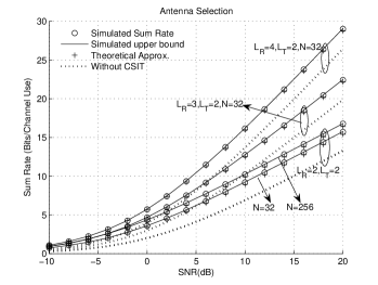
Figure 1: Antenna Selection: Sum Rate versus SNR.

Figure 2: General Beamforming: Sum Rate versus $R_{\mathrm{q}}$.

VI Conclusion

This paper proposes a joint quantization and feedback strategy for multiaccess MIMO systems with finite rate feedback. The effect of user choice is analyzed by extreme order statistics and the effect of eigen-channel vector quantization is quantified by analysis on the composite Grassmann manifold. By asymptotic random matrix theory, the sum rate is well approximated. Due to its simple implementation and solid performance analysis, the proposed scheme provides a benchmark for multiaccess MIMO systems with finite rate feedback.

-A Random Matrix Theory

Let $\mathbf{H}\in\mathbb{L}^{n\times m}$ be a standard Gaussian random matrix, where $\mathbb{L}$ is either $\mathbb{R}$ or $\mathbb{C}$. Let $\lambda_{1},\cdots,\lambda_{n}$ be the $n$ singular values of $\frac{1}{m}\mathbf{H}\mathbf{H}^{\dagger}$. Define the empirical distribution of the singular values

$$\mu_{n,\bm{\lambda}}\left(\lambda\right)\triangleq\frac{1}{n}\left|\left\{j:\;\lambda_{j}\leq\lambda\right\}\right|.$$

As $n,m\rightarrow\infty$ with $\frac{m}{n}\rightarrow\bar{m}\in\mathbb{R}^{+}$, the empirical measure converges to the Marc̆enko-Pastur law

$$d\mu_{\lambda}=\left(\left(1-\bar{m}\right)^{+}\delta\left(\lambda\right)+\frac{\bar{m}\sqrt{\left(\lambda-\lambda^{-}\right)^{+}\left(\lambda^{+}-\lambda\right)^{+}}}{2\pi\lambda}\right)\,d\lambda$$ (17)

almost surely, where $\lambda^{\pm}=\left(1\pm\sqrt{\frac{1}{\bar{m}}}\right)^{2}$ and $\left(x\right)^{+}=\max\left(x,0\right)$ (A good reference for this type of result is [23, Eq. (1.10)]). Define

$$\lambda_{t}^{-}\triangleq\begin{cases}0&\mathrm{if}\;\beta\geq 1\\ \lambda^{-}&\mathrm{if}\;\beta<1\end{cases}.$$

Consider as well a linear spectral statistic

$$g\left(\frac{1}{m}\mathbf{H}\mathbf{H}^{\dagger}\right)=\frac{1}{n}\sum_{i=1}^{n}g\left(\lambda_{i}\right).$$

If $g$ is Lipschitz on $\left[\lambda_{t}^{-},\lambda^{+}\right]$, then we also have that

$$\underset{\left(n,m\right)\rightarrow\infty}{\lim}g\left(\frac{1}{m}\mathbf{H}\mathbf{H}^{\dagger}\right)=\int g\left(\lambda\right)d\mu_{\lambda}$$

almost surely, see for example [28] for a modern approach.

The asymptotic properties of the maximum eigenvalue will figure into our analysis. Denote the largest eigenvalue by $\lambda_{1}$.

Proposition 1

Let $n,m\rightarrow\infty$ linearly with $\frac{m}{n}\rightarrow\bar{m}\in\mathbb{R}^{+}$.

1. $\lambda_{1}\rightarrow\lambda^{+}$ almost surely.

2. All moments of $\lambda_{1}$ also converge.

The almost sure convergence goes back to [29, 30]. The convergence of moments is implied by the tail estimates in [31]. A direct application of this proposition is that for $\forall A_{n}\subset\mathbb{R}^{n}$ such that $\mu_{n,\bm{\lambda}}\left(A_{n}\right)\rightarrow 0$, $\mathrm{E}_{\bm{\lambda}}\left[\lambda_{1},\;A_{n}\right]\rightarrow 0$.

Theorem 6

Let $\mathbf{H}\in\mathbb{L}^{n\times m}$ ($\mathbb{L}=\mathbb{R}/\mathbb{C}$) be standard Gaussian matrix and $\lambda_{i}$ be the $i^{\mathrm{th}}$ largest eigenvalue of $\frac{1}{m}\mathbf{H}\mathbf{H}^{\dagger}$.

1. Let $g\left(\lambda\right)=f\left(\lambda\right)\cdot\chi_{\left[a,\lambda^{+}\right]}\left(\lambda\right)$ for some $a<\lambda^{+}$ where $f\left(\lambda\right)$ is Lipschitz continuous on $\left[\lambda^{-},\lambda^{+}\right]$ and $\chi_{\left[a,\lambda^{+}\right]}\left(\lambda\right)$ is the indicator function on the set $\left[a,\lambda^{+}\right]$, then as $n,m\rightarrow\infty$ with $\frac{m}{n}\rightarrow\bar{m}\in\mathbb{R}^{+}$,

   $$\underset{\left(n,m\right)\rightarrow\infty}{\lim}\int g\left(\lambda\right)\cdot d\mu_{n,\bm{\lambda}}\left(\lambda\right)=\int g\left(\lambda\right)\cdot d\mu_{\lambda}$$

   almost surely and

   $$\underset{\left(n,m\right)\rightarrow\infty}{\lim}\mathrm{E}_{\bm{\lambda}}\left[\frac{1}{n}\sum_{i=1}^{n}g\left(\lambda_{i}\right)\right]=\int g\left(\lambda\right)\cdot d\mu_{\lambda}.$$

2. For $\forall a\in\left(\lambda_{t}^{-},\lambda^{+}\right)$,

   $$\mathrm{E}_{\bm{\lambda}}\left[\frac{1}{n}\left|\left\{\lambda_{i}:\;\lambda_{i}\geq a\right\}\right|\right]=\int_{a}^{\lambda^{+}}d\mu_{\lambda}.$$

3. For $\forall\tau\in\left(0,\min\left(1,\bar{m}\right)\right)$,

   $$\underset{\left(n,m\right)\rightarrow\infty}{\lim}\mathrm{E}\left[\frac{1}{n}\left(\sum_{1\leq i\leq n\tau}\lambda_{i}\right)\right]=\int_{a}^{\lambda^{+}}\lambda\cdot d\mu_{\lambda},$$

   where $a\in\left(\lambda^{-},\lambda^{+}\right)$ satisfies

   $$\tau=\int_{a}^{\lambda^{+}}d\mu_{\lambda}.$$

Proof:

1. Though $g\left(\lambda\right)$ is not Lipschitz continuous on $\left[\lambda_{t}^{-},\lambda^{+}\right]$, we are able to construct sequences of Lipschitz functions $g_{k}^{+}\left(\lambda\right)$ and $g_{k}^{-}\left(\lambda\right)$ such that $g_{k}^{\pm}\left(\lambda\right)$’s are Lipschitz continuous on $\left[\lambda_{t}^{-},\lambda^{+}\right]$ for all $k$, $g_{k}^{+}\left(\lambda\right)\geq g\left(\lambda\right)$ and $g_{k}^{-}\left(\lambda\right)\leq g\left(\lambda\right)$ for $\lambda\in\left[\lambda_{t}^{-},\lambda^{+}\right]$, and $g_{k}^{\pm}\left(\lambda\right)\rightarrow g\left(\lambda\right)$ pointwisely as $k\rightarrow\infty$. Due to their Lipschitz continuity, $g_{k}^{\pm}\left(\lambda\right)$’s are integrable with respect to $\mu_{\lambda}$. Then we have

   $$\underset{k\rightarrow\infty}{\lim}\underset{\left(n,m\right)\rightarrow\infty}{\lim}\int g_{k}^{-}\left(\lambda\right)\cdot d\mu_{n,\bm{\lambda}}\left(\lambda\right) \leq\underset{\left(n,m\right)\rightarrow\infty}{\lim}\int g\left(\lambda\right)\cdot d\mu_{n,\bm{\lambda}}\left(\lambda\right)$$

   $$\leq\underset{k\rightarrow\infty}{\lim}\underset{\left(n,m\right)\rightarrow\infty}{\lim}\int g_{k}^{+}\left(\lambda\right)\cdot d\mu_{n,\bm{\lambda}}\left(\lambda\right),$$

   while

   $$\underset{k\rightarrow\infty}{\lim}\underset{\left(n,m\right)\rightarrow\infty}{\lim}\int g_{k}^{-}\left(\lambda\right)\cdot d\mu_{n,\bm{\lambda}}\left(\lambda\right)=\underset{k\rightarrow\infty}{\lim}\int g_{k}^{-}\left(\lambda\right)\cdot d\mu\left(\lambda\right)=\int g\left(\lambda\right)\cdot d\mu\left(\lambda\right)$$

   and

   $$\underset{k\rightarrow\infty}{\lim}\underset{\left(n,m\right)\rightarrow\infty}{\lim}\int g_{k}^{+}\left(\lambda\right)\cdot d\mu_{n,\bm{\lambda}}\left(\lambda\right)=\int g\left(\lambda\right)\cdot d\mu\left(\lambda\right)$$

   almost surely. This proves the almost sure statement, and the convergence of the expectation follows from dominated convergence.

2. follows from the first part upon setting $g\left(\lambda\right)=\chi_{\left[a,\lambda^{+}\right]}\left(\lambda\right)$.

3. Since $a\in\left(\lambda^{-},\lambda^{+}\right)$, there exists an $\epsilon>0$ such that $\left(a-\epsilon,a+\epsilon\right)\subset\left(\lambda^{-},\lambda^{+}\right)$. For any $\delta>0$, define the events

   $$A_{n,a+\epsilon}=\left\{\bm{\lambda}:\;\frac{\left|\left\{\lambda_{i}:\;\lambda_{i}\geq a+\epsilon\right\}\right|}{n}<\tau\right\},$$

   $$A_{n,a-\epsilon}=\left\{\bm{\lambda}:\;\frac{\left|\left\{\lambda_{i}:\;\lambda_{i}\geq a-\epsilon\right\}\right|}{n}>\tau\right\},$$

   $$B_{n,a+\epsilon,\delta}=\left\{\bm{\lambda}:\;\left|\frac{1}{n}\sum_{\lambda_{i}\geq a+\epsilon}\lambda_{i}-\int_{a+\epsilon}^{\lambda^{+}}\lambda\cdot d\mu_{\lambda}\right|<\delta\right\},$$

   and

   $$B_{n,a-\epsilon,\delta}=\left\{\bm{\lambda}:\;\left|\frac{1}{n}\sum_{\lambda_{i}\geq a-\epsilon}\lambda_{i}-\int_{a-\epsilon}^{\lambda^{+}}\lambda\cdot d\mu_{\lambda}\right|<\delta\right\}.$$

   According to the first part of this theorem, it can be verified that $\forall\epsilon>0$, as $\left(n,m\right)\rightarrow\infty$, $\mu_{n,\bm{\lambda}}\left(A_{n,a+\epsilon}\right)\rightarrow 1$, $\mu_{n,\bm{\lambda}}\left(A_{n,a-\epsilon}\right)\rightarrow 1$, $\mu_{n,\bm{\lambda}}\left(B_{n,a+\epsilon,\delta}\right)\rightarrow 1$, and $\mu_{n,\bm{\lambda}}\left(B_{n,a-\epsilon,\delta}\right)\rightarrow 1$. Then for sufficiently large $n$,

   $$\mathrm{E}_{\bm{\lambda}}\left[\frac{1}{n}\sum_{i\leq n\tau}\lambda_{i}\right]$$

   $$\geq\mathrm{E}_{\bm{\lambda}}\left[\frac{1}{n}\sum_{i\leq n\tau}\lambda_{i},\;A_{n,a+\epsilon}\cap B_{n,a+\epsilon,\delta}\right]$$

   $$\overset{\left(a\right)}{\geq}\mathrm{E}_{\bm{\lambda}}\left[\frac{1}{n}\sum_{\lambda_{i}\geq a+\epsilon}\lambda_{i},\;A_{n,a+\epsilon}\cap B_{n,a+\epsilon,\delta}\right]$$

   $$\overset{\left(b\right)}{\geq}\mathrm{E}_{\bm{\lambda}}\left[\int_{a+\epsilon}^{\lambda^{+}}\lambda\cdot d\mu_{\lambda}-\delta,\;A_{n,a+\epsilon}\cap B_{n,a+\epsilon,\delta}\right]$$

   $$=\left(\int_{a+\epsilon}^{\lambda^{+}}\lambda\cdot d\mu_{\lambda}-\delta\right)\mu_{n,\bm{\lambda}}\left(A_{n,a+\epsilon}\cap B_{n,a+\epsilon,\delta}\right)$$

   $$\geq\left(\int_{a+\epsilon}^{\lambda^{+}}\lambda\cdot d\mu_{\lambda}-\delta\right)\left(1-\delta\right),$$ (18)

   where $\mathrm{E}\left[\cdot,A\right]$ denotes the expectation operation on the measurable set $A$, $\left(a\right)$ and $\left(b\right)$ follow from the definition of $A_{n,a+\epsilon}$ and $B_{n,a+\epsilon,\delta}$ respectively. Similarly, when $n$ is large enough,

   $$\mathrm{E}_{\bm{\lambda}}\left[\frac{1}{n}\sum_{i\leq n\tau}\lambda_{i}\right]$$

   $$\leq\mathrm{E}_{\bm{\lambda}}\left[\frac{1}{n}\sum_{i\leq n\tau}\lambda_{i},\;A_{n,a-\epsilon}\right]+\mathrm{E}_{\bm{\lambda}}\left[\lambda_{1},\;A_{n,a-\epsilon}^{c}\right]$$

   $$\overset{\left(c\right)}{\leq}\mathrm{E}_{\bm{\lambda}}\left[\frac{1}{n}\sum_{\lambda_{i}\geq a-\epsilon}\lambda_{i},\;A_{n,a-\epsilon}\right]+\delta$$

   $$\leq\mathrm{E}_{\bm{\lambda}}\left[\int_{a-\epsilon}^{\lambda^{+}}\lambda\cdot d\mu_{\lambda}+\delta,\;A_{n,a-\epsilon}\cap B_{n,a-\epsilon,\delta}\right]$$

   $$\quad\quad+\mathrm{E}_{\bm{\lambda}}\left[\lambda_{1},\;A_{n,a-\epsilon}\cap B_{n,a-\epsilon,\delta}^{c}\right]+\delta$$

   $$\overset{\left(d\right)}{\leq}\left(\int_{a-\epsilon}^{\lambda^{+}}\lambda\cdot d\mu_{\lambda}+\delta\right)\mu_{n,\bm{\lambda}}\left(A_{n,a-\epsilon}\cap B_{n,a-\epsilon,\delta}\right)+2\delta$$

   $$\leq\int_{a-\epsilon}^{\lambda^{+}}\lambda\cdot d\mu_{\lambda}+3\delta,$$ (19)

   where $\left(c\right)$ and $\left(d\right)$ are an application of Proposition 1. Now let $\delta\downarrow 0$ and then $\epsilon\downarrow 0$. Then we have proved that

   $$\underset{\left(n,m\right)\rightarrow\infty}{\lim}\mathrm{E}\left[\frac{1}{n}\left(\sum_{1\leq i\leq n\tau}\lambda_{i}\right)\right]=\int_{a}^{\lambda^{+}}\lambda\cdot d\mu_{\lambda}.$$

∎

-B Proof of Lemma 1

As the first step, we compute the asymptotic distribution and expectation of $X_{\left(n:n\right)}$. It can be verified that

$$1-F_{X}\left(y\right)=\int_{y}^{+\infty}f_{X}\left(x\right)dx=e^{-y}\left(\sum_{i=0}^{L-1}\frac{1}{i!}y^{i}\right),$$

and for $\forall a>0$,

$$\int_{a}^{+\infty}1-F_{X}\left(y\right)dy$$

$$=e^{-a}\left(\sum_{i=0}^{L-1}\frac{1}{i!}a^{i}+\sum_{i=0}^{L-2}\frac{1}{i!}a^{i}+\cdots+\sum_{i=0}^{0}\frac{1}{i!}a^{i}\right)$$

$$=e^{-a}\left(\sum_{i=0}^{L-1}\frac{L-i}{i!}a^{i}\right).$$

For $0<t<+\infty$, define

$$R\left(t\right)=\frac{\int_{t}^{+\infty}\left(1-F_{X}\left(y\right)\right)dy}{1-F_{X}\left(t\right)}.$$

Then

$$\underset{t\rightarrow+\infty}{\lim}R\left(t\right)=\underset{t\rightarrow+\infty}{\lim}\frac{\sum_{i=0}^{L-1}\frac{L-i}{i!}t^{i}}{\sum_{i=0}^{L-1}\frac{1}{i!}t^{i}}=1.$$ (20)

Now let

$$a_{n}=\inf\left\{x:1-F_{X}\left(x\right)\leq\frac{1}{n}\right\},$$

and

$$b_{n}=R\left(a_{n}\right)=\frac{\sum_{i=0}^{L-1}\frac{L-i}{i!}a_{n}^{i}}{\sum_{i=0}^{L-1}\frac{1}{i!}a_{n}^{i}}.$$

It can be verified that $a_{n}\overset{n\rightarrow\infty}{\longrightarrow}+\infty$, and that $b_{n}\overset{n\rightarrow\infty}{\longrightarrow}1$ by (20). Furthermore,

$$\underset{n\rightarrow\infty}{\lim}n\left[1-F_{X}\left(a_{n}+xb_{n}\right)\right]$$

$$=\underset{n\rightarrow\infty}{\lim}\frac{1-F_{X}\left(a_{n}+xb_{n}\right)}{1-F_{X}\left(a_{n}\right)}$$

$$=\underset{n\rightarrow\infty}{\lim}e^{-xb_{n}}\frac{\sum_{i=0}^{L-1}\frac{1}{i!}\left(a_{n}+xb_{n}\right)^{i}}{\sum_{i=0}^{L-1}\frac{1}{i!}\left(a_{n}\right)^{i}}$$

$$=e^{-x}.$$ (21)

Therefore, for all $x\in\mathbb{R}$ and sufficiently large $n$,

$$P\left(X_{\left(n:n\right)}<a_{n}+b_{n}x\right)$$

$$=\left[1-\frac{1}{n}n\left(1-F_{X}\left(a_{n}+b_{n}x\right)\right)\right]^{n}$$

$$=\exp\left(n\cdot\log\left(1-\frac{1}{n}e^{-x}\left(1+o\left(1\right)\right)\right)\right)$$

$$=\exp\left(-e^{-x}\left(1+o\left(1\right)\right)\right)$$

$$\overset{n\rightarrow\infty}{\longrightarrow}\exp\left(-e^{-x}\right).$$

This identifies the limiting distribution, and the tail is of sufficient decay to conclude that

$$\underset{n\rightarrow+\infty}{\lim}\mathrm{E}\left[\frac{X_{\left(n:n\right)}-a_{n}}{b_{n}}\right]=\int_{-\infty}^{+\infty}xde^{-e^{-x}}:=\mu_{1}.$$

Given the law of the first maxima $X_{\left(n:n\right)}$, the distribution and the expectation of the $k^{\mathrm{th}}$ maxima follow easily. With $z_{n}=a_{n}+b_{n}x$,

$$P\left(X_{\left(n-k+1:n\right)}\leq z_{n}\right)=\sum_{t=0}^{k-1}{n\choose t}\left(1-F_{X}\left(z_{n}\right)\right)^{t}F_{X}^{n-t}\left(z_{n}\right).$$

According to (21), ${n\choose t}\left(1-F_{X}\left(z_{n}\right)\right)^{t}\overset{n\rightarrow\infty}{\longrightarrow}\frac{1}{t!}e^{-tx}$ and $F_{X}^{n-t}\left(z_{n}\right)\overset{n\rightarrow\infty}{\longrightarrow}e^{-e^{-x}}$. Thus

$$P\left(\frac{X_{\left(n-k+1:n\right)}-a_{n}}{b_{n}}\leq x\right)\overset{n\rightarrow\infty}{\longrightarrow}\exp\left(-e^{-x}\right)\sum_{t=0}^{k-1}\frac{1}{t!}e^{-tx}.$$

Denote it by $H_{k}\left(x\right)$. The corresponding PDF is given by

$$h_{k}\left(x\right)=H_{k}^{{}^{\prime}}\left(x\right)=e^{-e^{-x}}\frac{1}{\left(k-1\right)!}e^{-kx}.$$ (22)

Define $\mu_{k}=\int_{-\infty}^{+\infty}xh_{k}\left(x\right)dx$. It can be verified that Evaluating $\mu_{k}^{x}$ gives an iterative formula

$$\mu_{k} =\frac{1}{\left(k-1\right)!}\int_{-\infty}^{+\infty}xe^{-kx}e^{-e^{-x}}dx$$

$$=0-\frac{1}{\left(k-1\right)!}\int_{-\infty}^{+\infty}e^{-e^{-x}}d\left(xe^{-(k-1)x}\right)$$

$$=\frac{1}{\left(k-2\right)!}\int_{-\infty}^{+\infty}xe^{-\left(k-1\right)x}e^{-e^{-x}}dx$$

$$\quad\quad-\frac{1}{\left(k-1\right)!}\int_{-\infty}^{+\infty}e^{-\left(k-1\right)x}e^{-e^{-x}}dx$$

$$=\mu_{k-1}^{x}-\frac{1}{k-1},$$

where the last step follows the fact that $\frac{1}{\left(k-2\right)!}e^{-\left(k-1\right)}\exp\left(-e^{-x}\right)$ is the asymptotic pdf of $\left(k-1\right)^{\mathrm{th}}$ maxima. Therefore,

$$\underset{n\rightarrow+\infty}{\lim}\mathrm{E}\left[\frac{X_{\left(n-k+1:n\right)}-a_{n}}{b_{n}}\right]=\mu_{k}=\mu_{1}-\sum_{i=1}^{k-1}\frac{1}{i}.$$

and so also,

$$\underset{n\rightarrow+\infty}{\lim}\mathrm{E}\left[\frac{\sum_{k=1}^{s}X_{\left(n-k+1:n\right)}-sa_{n}}{b_{n}}\right]=\sum_{k=1}^{s}\mu_{k}=s\mu_{1}-\sum_{i=1}^{s}\frac{s-i}{i}.$$

-C Proof of Theorem 1

The proof of Theorem 1 is similar to that of Theorem 2 in our earlier paper [11]; the difference being that the composite Grassmann manifold is of interest here while the “single” Grassmann manifold is the focus in that work. The key step of this proof is the volume calculation of a small ball in the composite Grassmann manifold. Given the volume formula, the upper and lower bounds follow from the exact arguments in [11].

A metric ball in $\mathcal{G}_{n,p}^{\left(m\right)}\left(\mathbb{L}\right)$ centered at $P^{\left(m\right)}\in\mathcal{G}_{n,p}^{\left(m\right)}\left(\mathbb{L}\right)$ with radius $\delta\geq 0$ is defined as

$$B_{P^{\left(m\right)}}\left(\delta\right):=\left\{Q^{\left(m\right)}\in\mathcal{G}_{n,p}^{\left(m\right)}\left(\mathbb{L}\right):\;d_{c}\left(P^{\left(m\right)},Q^{\left(m\right)}\right)\leq\delta\right\}.$$

The volume of $B_{P^{\left(m\right)}}\left(\delta\right)$ as the probability of an isotropically distributed $Q^{\left(m\right)}\in\mathcal{G}_{n,p}^{\left(m\right)}\left(\mathbb{L}\right)$ in this ball:

$$\mu\left(B_{P^{\left(m\right)}}\left(\delta\right)\right):=\Pr\left(Q^{\left(m\right)}\in B_{P^{\left(m\right)}}\left(\delta\right)\right).$$

Since $\mu\left(B_{P^{\left(m\right)}}\left(\delta\right)\right)$ is independent of the choice of the center $P^{\left(m\right)}$, we simply denote it by $\mu^{\left(m\right)}\left(\delta\right)$. We have:

Theorem 7

When $\delta\leq 1$,

$$\mu^{\left(m\right)}\left(\delta\right)=\frac{\Gamma^{m}\left(\frac{t}{2}+1\right)}{\Gamma\left(m\frac{t}{2}+1\right)}c_{n,p,p,\beta}^{m}\delta^{mt},$$ (23)

where $c_{n,p,p,\beta}$ and $t$ are defined in Lemma 4.

Proof:

Let us drop the subscript of $c_{n,p,p,\beta}$ during the proof. In [11], we proved that for a single Grassmann manifold, $\mu^{\left(1\right)}\left(d_{c}^{2}\leq x\right)=\mu^{\left(1\right)}\left(\sqrt{x}\right)=cx^{\frac{t}{2}}\left(1+O\left(x\right)\right)$ when $x\leq 1$, and it can be verified that

$$d\mu\left(d_{c}^{2}\leq x\right)=\frac{t}{2}cx^{\frac{t}{2}-1}\left(1+O\left(x\right)\right)\cdot dx.$$

By the definition of the volume, $d\mu^{\left(2\right)}\left(x\right)/dx$ is a convolution of $d\mu\left(x\right)/dx$ and $d\mu\left(x\right)/dx$. So,

$$\frac{d\mu^{\left(2\right)}\left(x\right)}{dx} =\int_{0}^{x}\frac{t^{2}}{4}c^{2}\tau^{\frac{t}{2}-1}\left(x-\tau\right)^{\frac{t}{2}-1}\left(1+O\left(\tau\right)\right)\left(1+O\left(x-\tau\right)\right)d\tau$$

$$\overset{\left(a\right)}{=}\frac{t^{2}}{4}c^{2}x^{t-1}\int_{0}^{1}y^{\frac{t}{2}-1}\left(1-y\right)^{\frac{t}{2}-1}\left(1+O\left(xy\right)+O\left(x\left(1-y\right)\right)\right)dy$$

$$=\frac{t^{2}}{4}c^{2}x^{t-1}\frac{\Gamma\left(\frac{t}{2}\right)\Gamma\left(\frac{t}{2}\right)}{\Gamma\left(t\right)}\left(1+O\left(x\right)\right),$$

where $\left(a\right)$ follows from the variable change $\tau=xy$. A calculation produces

$$\mu^{\left(2\right)}\left(d_{c}^{2}\leq x\right)=\frac{\Gamma\left(\frac{t}{2}+1\right)\Gamma\left(\frac{t}{2}+1\right)}{\Gamma\left(t+1\right)}c^{2}x^{t}\left(1+O\left(x\right)\right).$$

By mathematical induction, we reach (23). Note that $\delta\leq 1$ is required in every step. ∎

Based on the volume formula, an upper bound on the distortion rate function $D^{*}\left(K\right)$ on the composite Grassmann manifold

$$D^{*}\left(K\right)\leq\frac{2}{mt}\Gamma\left(\frac{2}{mt}\right)\frac{\Gamma^{\frac{2}{mt}}\left(m\frac{t}{2}+1\right)}{\Gamma^{\frac{2}{t}}\left(\frac{t}{2}+1\right)}c_{n,p,p,\beta}^{-\frac{2}{t}}2^{-\frac{2\log_{2}K}{mt}}\left(1+o\left(1\right)\right)$$

is derived by calculating the average distortion of random codes (see [11] for details). Furthermore, by the sphere packing/covering argument (again see [11] for details), the lower bound

$$\frac{mt}{mt+2}\frac{\Gamma^{\frac{2}{mt}}\left(mt+1\right)}{\Gamma^{\frac{2}{t}}\left(t+1\right)}c_{n,p,p,\beta}^{-\frac{2}{t}}2^{-\frac{2\log_{2}K}{mt}}\left(1+o\left(1\right)\right)\leq D^{*}\left(K\right)$$

is arrived at. Theorem 1 is proved.

-D Proof of Theorem 5

The key step is to prove that $\mathrm{E}_{\mathcal{B},\mathbf{H}}\left[\mathbf{V}_{k}^{\dagger}\mathbf{b}_{k}\mathbf{b}_{k}^{\dagger}\mathbf{V}_{k}\right]=\mathrm{diag}\left[\frac{\gamma}{s},\frac{s-\gamma}{s\left(L_{T}-1\right)},\cdots,\frac{s-\gamma}{s\left(L_{T}-1\right)}\right]$, where $\mathbf{V}_{k}$ is from the singular value decomposition $\mathbf{H}_{\left(k\right)}=\mathbf{U}_{k}\mathbf{\Lambda}_{k}\bar{\mathbf{V}}_{k}^{\dagger}$. Let $\mathbf{V}_{k}=\left[\mathbf{v}_{k}\bar{\mathbf{V}}_{k}\right]$ where $\bar{\mathbf{V}}_{k}\in\mathbb{C}^{L_{T}\times\left(L_{T}-1\right)}$ is composed of all the columns of $\mathbf{V}_{k}$ except $\mathbf{v}_{k}$. Let $\mathbf{V}=\left[\mathbf{v}_{1}\cdots\mathbf{v}_{s}\right]$. Recall our feedback function $\varphi\left(\mathbf{V}\right)$ in (13) and definition of $\gamma$ in (15). Then the fact that

$$\mathrm{E}_{\mathcal{B},\mathbf{H}}\left[\mathbf{v}_{k}^{\dagger}\mathbf{b}_{k}\mathbf{b}_{k}^{\dagger}\mathbf{v}_{k}\right]=\frac{\gamma}{s}$$

is implied by the following lemma.

Lemma 5

Let $\mathbf{V}\in\mathcal{M}_{L_{T},1}^{\left(s\right)}$ be isotropically distributed and $\mathcal{B}\subset\mathcal{M}_{L_{T},1}^{\left(s\right)}$ be randomly generated from the isotropic distribution. Let $\mathbf{B}=\varphi\left(\mathbf{V}\right)$ where $\varphi\left(\cdot\right)$ is given in (13) and $\gamma$ is given by (15). Then

$$\mathrm{E}_{\mathcal{B},\mathbf{V}}\left[\mathbf{V}^{\dagger}\mathbf{B}\mathbf{B}^{\dagger}\mathbf{V}\right]=\frac{\gamma}{s}\mathbf{I}_{s}.$$

Proof:

Let $\mathbf{Z}=\mathrm{E}_{\mathcal{B},\mathbf{V}}\left[\mathbf{V}^{\dagger}\mathbf{B}\mathbf{B}^{\dagger}\mathbf{V}\right]$. For any $\theta\in\left[0,2\pi\right)$, let $\mathbf{A}_{k}=\mathrm{diag}\left[1,\cdots,1,e^{j\theta},1,\cdots,1\right]$ be obtained by replacing the $k^{\mathrm{th}}$ diagonal element of $\mathbf{I}$ with $e^{j\theta}$. It can be verified that $\mathbf{V}\mathbf{A}_{k}\in\mathcal{M}_{L_{T},1}^{\left(s\right)}$ is isotropically distributed, and $\varphi\left(\mathbf{V}\mathbf{A}_{k}\right)=\varphi\left(\mathbf{V}\right)=\mathbf{B}$. We have

$$\mathbf{Z} =\mathrm{E}_{\mathcal{B},\mathbf{V}\mathbf{A}_{k}}\left[\mathbf{A}_{k}^{\dagger}\mathbf{V}^{\dagger}\mathbf{B}\mathbf{B}^{\dagger}\mathbf{V}\mathbf{A}_{k}\right]$$

$$=\mathbf{A}_{k}^{\dagger}\mathrm{E}_{\mathcal{B},\mathbf{V}}\left[\mathbf{V}^{\dagger}\mathbf{B}\mathbf{B}^{\dagger}\mathbf{V}\right]\mathbf{A}_{k}$$

$$=\mathbf{A}_{k}^{\dagger}\mathbf{Z}\mathbf{A}_{k},$$

where the first equality is obtained by changing the variable from $\mathbf{V}$ to $\mathbf{VA}_{k}$, and the second equality is obtained by replacing the measure of $\mathbf{VA}_{k}$ with the measure of $\mathbf{V}$. Then $\left(\mathbf{Z}\right)_{k,j}=e^{-j\theta}\left(\mathbf{Z}\right)_{k,j}$ for $j\neq k$, which is only possible if $\left(\mathbf{Z}\right)_{k,j}=0$. Therefore, $\mathbf{Z}$ is a diagonal matrix.

Now let $\mathbf{P}\in\mathbb{R}^{s\times s}$ be a permutation matrix generated by permutating rows/columns of the identity matrix. Let $\mathcal{B}\mathbf{P}=\left\{\mathbf{BP}:\;\mathbf{B}\in\mathcal{B}\right\}$. Then $\mathbf{VP}\in\mathcal{M}_{L_{T},1}^{\left(s\right)}$ and $\mathbf{BP}\in\mathcal{M}_{L_{T},1}^{\left(s\right)}$ are isotropically distributed. It can be verified that $\varphi_{\mathcal{B}\mathbf{P}}\left(\mathbf{VP}\right)=\mathbf{BP}=\varphi_{\mathcal{B}}\left(\mathbf{V}\right)\mathbf{P}$, where the subscript $\varphi$ emphasizes the choice of codebook. Then,

$$\mathbf{Z} =\mathrm{E}_{\mathcal{B}\mathbf{P},\mathbf{VP}}\left[\left(\mathbf{VP}\right)^{\dagger}\varphi_{\mathcal{B}\mathbf{P}}\left(\mathbf{VP}\right)\varphi_{\mathcal{B}\mathbf{P}}\left(\mathbf{VP}\right)^{\dagger}\left(\mathbf{VP}\right)\right]$$

$$=\mathbf{P}^{\dagger}\mathrm{E}_{\mathcal{B}\mathbf{P},\mathbf{V}}\left[\mathbf{V}^{\dagger}\varphi_{\mathcal{B}\mathbf{P}}\left(\mathbf{VP}\right)\varphi_{\mathcal{B}\mathbf{P}}\left(\mathbf{VP}\right)^{\dagger}\mathbf{V}\right]\mathbf{P}$$

$$=\mathbf{P}^{\dagger}\mathrm{E}_{\mathcal{B}\mathbf{P},\mathbf{V}}\left[\mathbf{V}^{\dagger}\varphi_{\mathcal{B}}\left(\mathbf{V}\right)\mathbf{P}\mathbf{P}^{\dagger}\varphi_{\mathcal{B}}\left(\mathbf{V}\right)^{\dagger}\mathbf{V}\right]\mathbf{P}$$

$$=\mathbf{P}^{\dagger}\mathrm{E}_{\mathcal{B},\mathbf{V}}\left[\mathbf{V}^{\dagger}\varphi_{\mathcal{B}}\left(\mathbf{V}\right)\varphi_{\mathcal{B}}\left(\mathbf{V}\right)^{\dagger}\mathbf{V}\right]\mathbf{P}$$

$$=\mathbf{P}^{\dagger}\mathbf{Z}\mathbf{P},$$

where the first equality is obtained by variables change, and the second and fourth equality follows from measure replacement. It follows that $\left(\mathbf{Z}\right)_{i,i}=\left(\mathbf{Z}\right)_{j,j}$ for $1\leq i,j\leq s$.

Finally, $\mathbf{Z}=\frac{\gamma}{s}\mathbf{I}$ follows from the fact that $\mathrm{tr}\left(\mathbf{Z}\right)=\mathrm{E}\left[\mathrm{tr}\left(\mathbf{V}^{\dagger}\mathbf{B}\mathbf{B}^{\dagger}\mathbf{V}\right)\right]=\gamma$. ∎

We evaluate

$$\mathrm{E}\left[\mathbf{V}_{k}^{\dagger}\mathbf{b}_{k}\mathbf{b}_{k}^{\dagger}\mathbf{V}_{k}\right]=\left[\begin{array}[]{cc}\mathrm{E}\left[\mathbf{v}_{k}^{\dagger}\mathbf{b}_{k}\mathbf{b}_{k}^{\dagger}\mathbf{v}_{k}\right]&\mathrm{E}\left[\mathbf{v}_{k}^{\dagger}\mathbf{b}_{k}\mathbf{b}_{k}^{\dagger}\bar{\mathbf{V}}_{k}\right]\\ \mathrm{E}\left[\bar{\mathbf{V}}_{k}^{\dagger}\mathbf{b}_{k}\mathbf{b}_{k}^{\dagger}\mathbf{v}_{k}\right]&\mathrm{E}\left[\bar{\mathbf{V}}_{k}^{\dagger}\mathbf{b}_{k}\mathbf{b}_{k}^{\dagger}\bar{\mathbf{V}}_{k}\right]\end{array}\right].$$

For any unitary matrix $\mathbf{U}_{r}\in\mathbb{C}^{\left(L_{T}-1\right)\times\left(L_{T}-1\right)}$, $\left[\mathbf{v}_{k},\bar{\mathbf{V}}_{k}\mathbf{U}\right]$ is also isotropically distributed. Employ the method in the proof of Lemma 5 to find that

$$\mathrm{E}\left[\mathbf{v}_{k}^{\dagger}\mathbf{b}_{k}\mathbf{b}_{k}^{\dagger}\bar{\mathbf{V}}_{k}\right]=\mathrm{E}\left[\mathbf{v}_{k}^{\dagger}\mathbf{b}_{k}\mathbf{b}_{k}^{\dagger}\bar{\mathbf{V}}_{k}\right]\mathbf{U},$$

$$\mathrm{and}\quad\mathrm{E}\left[\bar{\mathbf{V}}_{k}^{\dagger}\mathbf{b}_{k}\mathbf{b}_{k}^{\dagger}\bar{\mathbf{V}}_{k}\right]=\mathbf{U}^{\dagger}\mathrm{E}\left[\bar{\mathbf{V}}_{k}^{\dagger}\mathbf{b}_{k}\mathbf{b}_{k}^{\dagger}\bar{\mathbf{V}}_{k}\right]\mathbf{U}.$$

Therefore, $\mathrm{E}\left[\mathbf{v}_{k}^{\dagger}\mathbf{b}_{k}\mathbf{b}_{k}^{\dagger}\bar{\mathbf{V}}_{k}\right]=\mathbf{o}^{\dagger}$ and $\mathrm{E}\left[\bar{\mathbf{V}}_{k}^{\dagger}\mathbf{b}_{k}\mathbf{b}_{k}^{\dagger}\bar{\mathbf{V}}_{k}\right]=c\mathbf{I}_{L_{T}-1}$ for some constant $c$. Note that $\mathrm{E}\left[\mathbf{v}_{k}^{\dagger}\mathbf{b}_{k}\mathbf{b}_{k}^{\dagger}\mathbf{v}_{k}\right]=\frac{\gamma}{s}$ and $\mathrm{E}\left[\mathrm{tr}\left(\mathbf{V}_{k}^{\dagger}\mathbf{b}_{k}\mathbf{b}_{k}^{\dagger}\mathbf{V}_{k}\right)\right]=1$. Hence, $c=\frac{s-\gamma}{s\left(L_{T}-1\right)}$ and $\mathrm{E}\left[\mathbf{V}_{k}^{\dagger}\mathbf{b}_{k}\mathbf{b}_{k}^{\dagger}\mathbf{V}_{k}\right]=\mathrm{diag}\left[\frac{\gamma}{s},\frac{s-\gamma}{s\left(L_{T}-1\right)},\cdots,\frac{s-\gamma}{s\left(L_{T}-1\right)}\right]$.

Finally,

$$\mathrm{E}_{\mathcal{B}}\left[\eta\right] =\frac{1}{sL_{R}}\mathrm{E}_{\mathcal{B},\mathbf{H}}\left[\sum_{k=1}^{s}n_{k}^{2}\right]$$

$$=\frac{1}{sL_{R}}\sum_{k=1}^{s}\mathrm{E}_{\mathcal{B},\mathbf{H}}\left[\mathrm{tr}\left(\mathbf{H}_{\left(k\right)}\mathbf{b}_{k}\mathbf{b}_{k}^{\dagger}\mathbf{H}_{\left(k\right)}^{\dagger}\right)\right]$$

$$=\frac{1}{sL_{R}}\sum_{k=1}^{s}\mathrm{tr}\left(\mathrm{E}_{\mathcal{B},\mathbf{H}}\left[\mathbf{V}_{k}^{\dagger}\mathbf{b}_{k}\mathbf{b}_{k}^{\dagger}\mathbf{V}_{k}\right]\mathrm{E}_{\mathbf{H}}\left[\mathbf{\Lambda}_{k}^{\dagger}\mathbf{\Lambda}_{k}\right]\right)$$

$$=\frac{1}{sL_{R}}\sum_{k=1}^{s}\left(\frac{\gamma}{s}\zeta_{1}\mathrm{E}_{\mathbf{H}}\left[n_{\left(k\right)}^{2}\right]+\frac{s-\gamma}{s}\frac{\left(1-\zeta_{1}\right)\mathrm{E}_{\mathbf{H}}\left[n_{\left(k\right)}^{2}\right]}{L_{T}-1}\right)$$

$$=\frac{1}{L_{R}}\left(\frac{\gamma}{s}\zeta_{1}+\frac{s-\gamma}{s}\frac{1-\zeta_{1}}{L_{T}-1}\right)\bar{n}_{\left(\cdot\right)}^{2},$$

where the third line follows from the fact that $\mathbf{\Lambda}_{k}$ is independent of $\mathbf{V}_{k}$ and $\mathbf{b}_{k}$.

References

- [1] I. Telatar, “Capacity of multi-antenna gaussian channels,” Euro. Trans. Telecommun., vol. 10, pp. 585–595, 1999.
- [2] K. K. Mukkavilli, A. Sabharwal, E. Erkip, and B. Aazhang, “On beamforming with finite rate feedback in multiple-antenna systems,” IEEE Trans. Info. Theory, vol. 49, no. 10, pp. 2562–2579, 2003.
- [3] D. J. Love, J. Heath, R. W., and T. Strohmer, “Grassmannian beamforming for multiple-input multiple-output wireless systems,” IEEE Trans. Info. Theory, vol. 49, no. 10, pp. 2735–2747, 2003.
- [4] J. Zheng, E. R. Duni, and B. D. Rao, “Analysis of multiple-antenna systems with finite-rate feedback using high-resolution quantization theory,” IEEE Trans. Signal Processing, vol. 55, no. 4, pp. 1461–1476, 2007.
- [5] W. Santipach, Y. Sun, and M. L. Honig, “Benefits of limited feedback for wireless channels,” in Proc. Allerton Conf. on Commun., Control, and Computing, 2003.
- [6] J. C. Roh and B. D. Rao, “MIMO spatial multiplexing systems with limited feedback,” in Proc. IEEE International Conference on Communications (ICC), 2005.
- [7] D. Love and J. Heath, R.W., “Limited feedback unitary precoding for spatial multiplexing systems,” IEEE Trans. Info. Theory, vol. 51, no. 8, pp. 2967–2976, 2005.
- [8] B. Mondal, R. W. H. Jr., and L. W. Hanlen, “Quantization on the Grassmann manifold: Applications to precoded MIMO wireless systems,” in Proc. IEEE International Conference on Acoustics, Speech, and Signal Processing (ICASSP), 2005, pp. 1025–1028.
- [9] W. Dai, Y. Liu, B. Rider, and V. Lau, “On the information rate of MIMO systems with finite rate channel state feedback and power on/off strategy,” in Proc. IEEE International Symposium on Information Theory (ISIT), 2005, pp. 1549–1553.
- [10] W. Dai, Y. Liu, V. K. N. Lau, and B. Rider, “On the information rate of MIMO systems with finite rate channel state feedback using beamforming and power on/off strategy,” IEEE Trans. Info. Theory, submitted, 2005. [Online]. Available: http://arxiv.org/abs/cs/0603040
- [11] W. Dai, Y. Liu, and B. Rider, “Quantization bounds on Grassmann manifolds and applications to MIMO systems,” IEEE Trans. Inform. Theory, vol. 54, no. 3, pp. 1108–1123, March 2008.
- [12] T. M. Cover and J. A. Thomas, Elements of Information Theory, 2nd ed. John Wiley and Sons, 2006.
- [13] S. Vishwanath, N. Jindal, and A. Goldsmith, “Duality, achievable rates, and sum-rate capacity of gaussian mimo broadcast channels,” Information Theory, IEEE Transactions on, vol. 49, no. 10, pp. 2658–2668, 2003.
- [14] M. Sharif and B. Hassibi, “On the capacity of mimo broadcast channels with partial side information,” Information Theory, IEEE Transactions on, vol. 51, no. 2, pp. 506–522, 2005.
- [15] N. Jindal, “MIMO broadcast channels with finite-rate feedback,” IEEE Trans. Info. Theory, vol. 52, no. 11, pp. 5045–5060, 2006.
- [16] W. Dai, Y. Liu, and B. Rider, “How many users should be turned on in a multi-antenna broadcast channel?” in Conf. on Info. Sciences and Systems (CISS), 2007.
- [17] V. K. N. Lau, L. Youjian, and T. A. Chen, “Capacity of memoryless channels and block-fading channels with designable cardinality-constrained channel state feedback,” IEEE Trans. Info. Theory, vol. 50, no. 9, pp. 2038–2049, 2004.
- [18] J. Galambos, The asymptotic theory of extreme order statistics, 2nd ed. Roberte E. Krieger Publishing Company, 1987.
- [19] R. J. Muirhead, Aspects of multivariate statistical theory. New York: John Wiley and Sons, 1982.
- [20] J. H. Conway, R. H. Hardin, and N. J. A. Sloane, “Packing lines, planes, etc., packing in Grassmannian spaces,” Exper. Math., vol. 5, pp. 139–159, 1996.
- [21] A. Haar, “Der Massbegriff in der Theorie der kontinuierlichen Gruppen,” Ann. Math., vol. 34, 1933.
- [22] W. Dai, Y. Liu, and B. Rider, “Quantization bounds on Grassmann manifolds of arbitrary dimensions and MIMO communications with feedback,” in IEEE Global Telecommunications Conference (GLOBECOM), 2005.
- [23] A. M. Tulino and S. Verd , “Random matrices and wireless communications,” Foundations and Trends in Communications and Information Theory, vol. 1, no. 1, June 2004.
- [24] S. Verdu and S. Shamai, “Spectral efficiency of cdma with random spreading,” Information Theory, IEEE Transactions on, vol. 45, no. 2, pp. 622–640, 1999.
- [25] T. M. Cover and J. A. Thomas, Elements of Information Theory. New York: John Wiley and Sons, 1991.
- [26] A. Edelman and N. R. Rao, “Random matrix theory,” Acta Numerica, vol. 14, pp. 233–297, 2005.
- [27] A. T. James, “Normal multivariate analysis and the orthogonal group,” Ann. Math. Statist., vol. 25, no. 1, pp. 40 – 75, 1954.
- [28] A. Guionnet and O. Zeitouni, “Concentration of the spectral measure for large matrices,” Electronic Communications in Probability, vol. 5, pp. 119–136, 2000.
- [29] Z. D. Bai, Y. Q. Yin, and P. R. Krishnaih, “On limit of the largest eigenvalue of the large dimensional sample covariance matrix,” Probability Theory and Related Fields, vol. 78, pp. 509–521, 1988.
- [30] Z. D. Bai and Y. Yin, “Limit of the smallest eigenvalue of a large dimensional sample covariance matrix,” Annals of Probability, vol. 21, pp. 1275–1294, 1993.
- [31] M. Ledoux, “Differential operators and spectral distributions of invariant ensembles from the classical orthogonal polynomials. the continuous case,” Electron. J. Probab, vol. 10, no. 34, pp. 1116–1146, 2005.