Self Similar Renormalization Group Applied to Diffusion in non-Gaussian Potentials

Abstract

We study the problem of the computation of the effective diffusion constant of a Brownian particle diffusing in a random potential which is given by a function $V(\phi)$ of a Gaussian field $\phi$. A self similar renormalization group analysis is applied to a mathematically related problem of the effective permeability of a random porous medium from which the diffusion constant of the random potential problem can be extracted. This renormalization group approach reproduces practically all known exact results in one and two dimensions. The results are confronted with numerical simulations and we find that their accuracy is good up to points well beyond the expected perturbative regime. The results obtained are also tentatively applied to interacting particle systems without disorder and we obtain expressions for the self-diffusion constant in terms of the excess thermodynamic entropy. This result is of a form that has commonly been used to fit the self diffusion constant in molecular dynamics simulations.

1 Introduction

In this paper we will consider the late time diffusion constant associated with a Brownian or Langevin particle, in D dimensions, advected by a velocity field which is given by the gradient of a random potential. The explicit Langevin equation studied is:

$${d\mathbf{X}\over dt}=\nabla V\left(\phi(\mathbf{X})\right)+{\mathbf{\eta}}(t)$$ (1)

where the local potential $V$ is itself a function of a Gaussian random field $\phi$. In general (up to an overall rescaling of time) the potential $V$ can be written and

$$V(\phi)=-\beta\nu(\phi)$$ (2)

where $\beta$ is the inverse temperature and $\nu$ is the physical potential acting on the tracer particle. In this formulation $\eta(t)$ is a Gaussian white noise of zero mean with correlation function

$$\langle\eta_{i}(t)\eta_{j}(t^{\prime})\rangle=2\delta_{ij}\delta(t-t^{\prime}).$$ (3)

Therefore when $V$ is not a linear function of $\phi$ the advecting potential is non-Gaussian. The case of diffusion in purely Gaussian potentials has been extensively studied in the literature [1, 2, 3] but the non-Gaussian case has received much less attention. The Gaussian case has been studied within a variety of approximation schemes and among these schemes the most successful has been the self-similar renormalization group method which reproduces exact results in one and two dimensions and which in addition is in excellent agreement with numerical simulations in three dimensions [1, 2, 3]. The case where $V$ is the square of the gradient of a Gaussian potential arises naturally in the case of dipoles diffusing in a random electric field (in the limit where the dipole moment equilibriates very quickly in its local field compared to the time-scales over which the diffusion of its centre of mass occurs) [4]. The authors of this paper have examined the case

$$\nu=\alpha{\phi^{2}\over 2}$$ (4)

in one dimension [5] , where the diffusion constant can be calculated exactly. In this case it can be shown that there is a critical temperature at which the diffusion constant vanishes. Below this temperature the diffusion is anomalous (more precisely sub-diffusive) and the exponent associated with anomalous diffusion can be computed. The exact results of [5] show that the transport properties (the exponent associated with the anomalous diffusion) agree with those obtained by a straightforward mapping onto a trap model whose trapping time statistics can be deduced from the statistics of the field $\phi$ and the Arrhenius law. There have also been some studies of diffusion in (non-Gaussian) potentials generated by the potentials due to a distribution of randomly distributed particles which interact with the potential via a fixed deterministic potential [6, 7].

A naive application of the self-similar renormalization group to this model at the one-loop level is not sensitive to the non-Gaussian statistics of the random potential and fails to predict the dynamical phase transition associated with the passage from normal to sub-diffusive transport. In this paper we reformulate the self-similar renormalization group approach in such away that the results for the Gaussian case are unchanged but we reproduce all known exact results in one and two dimensions. In addition we show that the approach works well in other cases by comparison with numerical simulations, it predicts the dynamical transition, when there is one, and works reasonably well outside the perturbative regime. The basis of our analysis relies on the mapping of diffusion in the random potential to diffusion in a medium of random diffusivity, this is mainly done as it simplifies the resulting renormalization group flow. Interestingly, as a biproduct our analysis recovers an approximate results often used in the computation of the effective permeability of random porous media [3, 8, 9, 10, 11, 12]

The underlying Gaussian potential we shall study will be assumed to have a short range correlation of the from

$$\langle\phi(\mathbf{x})\phi(\mathbf{y})\rangle=\Delta(\mathbf{x}-\mathbf{y})$$ (5)

In a translationally invariant and isotropic system the long-time behavior of the mean-squared displacement of the process $\mathbf{X}$ described by equation (1) is

$$\langle\mathbf{X}^{2}\rangle\sim 2D\kappa_{e}t$$ (6)

where $\kappa_{e}$ is thus the long-time effective diffusion constant of the problem. The Fokker-Planck equation describing the evolution of the probability density function (pdf) for $\mathbf{X}$ is:

$${\partial P\over\partial t}=\nabla\cdot\left(\nabla P-P\nabla V(\phi)\right)$$ (7)

The problem of diffusion in a medium of random local diffusivity $\kappa=\exp(V(\phi))$ is described by the Fokker-Planck equation

$${\partial P\over\partial t}=\nabla\cdot\exp\left(V(\phi)\right)\nabla P.$$ (8)

The corresponding stochastic differential equation is

$${d\mathbf{X}\over dt}=\exp\left(V\left(\phi(\mathbf{X})\right)\right)\nabla V\left(\phi(\mathbf{X})\right)+\sqrt{\exp\left(V\left(\phi(\mathbf{X})\right)\right)}{\mathbf{\eta}}(t).$$ (9)

Again under the assumptions of time-translational invariance and isotropy the late-time behaviour of a Brownian tracer particle described by the above Fokker-Planck equation is

$$\langle\mathbf{X}^{2}\rangle\sim 2D\kappa_{e}^{(p)}t$$ (10)

where $\kappa_{p}$ is the associated long-time diffusion constant. The effective diffusion constant $\kappa_{e}^{(p)}$ is also the effective permeability of a random porous medium where fluid flow is described by Darcy’s law and if $\kappa$ is interpreted as a local dielectric constant then $\kappa^{(p)}_{e}$ is the effective dielectric constant of the medium (see the review [3]). The effective late-time diffusion constants of the two Fokker-Planck equations (7) (gradient flow) and (8) (fluctuating diffusivity) are in fact related via

$$\kappa={\kappa_{p}\over\langle\exp\left(V(\phi)\right)\rangle},$$ (11)

a result which can be shown in a number of different ways [3, 7, 13]. The effective diffusivity can be computed from a statics problem. If one considers the Green’s function for the random diffusivity problem

$$\nabla\cdot\exp\left(V(\phi)\right)\nabla G=-\delta(\mathbf{x}),$$ (12)

the effective diffusivity can be read off from the long-distance behavior of the Green’s function or equivalently the short wave-length behaviour of its Fourier transform:

$$\langle{\tilde{G}}(\mathbf{k})\rangle\sim{1\over\kappa_{e}^{(p)}\mathbf{k}^{2}}$$ (13)

which means that on suitably large length scales Green’s function reads

$$G^{-1}\sim-\kappa_{e}^{(p)}\nabla^{2}.$$ (14)

Note we have dropped the disorder average as we shall assume that $\kappa_{e}^{(p)}$is self-averaging.

2 Renormalization Group Approach

The basic idea of the self-similar renormalization group [1, 2] is to average out the short distance components of the random field $\phi$ down to some wave-length $\Lambda$ and then to write an effective diffusion equation, of the same structural form, describing the transport at length scales greater than $1/\Lambda$.

The Gaussian field is decomposed by defining

$$\phi_{\Lambda}(\mathbf{x})=\int_{|\mathbf{k}|<\Lambda}{d\mathbf{k}\over(2\pi)^{D}}\exp(i\mathbf{k}\cdot\mathbf{x})\tilde{\phi}(\mathbf{k})$$ (15)

where $\Lambda$ is an upper ultraviolet scale which is initially infinite. We define a slice of the field $\phi$ at inverse length scale $\Lambda$

$$\delta\phi_{\Lambda}(\mathbf{x})=\int_{\Lambda-\delta\Lambda|\mathbf{k}|<\Lambda}{d\mathbf{k}\over(2\pi)^{D}}\exp(i\mathbf{k}\cdot\mathbf{x})\tilde{\phi}(\mathbf{k})$$ (16)

The self-similar renormalization group process proceeds by integrating out the slice of the field $\delta\phi$ whilst assuming that the remaining part of the field $\phi_{\Lambda-\delta\Lambda}$ can be treated as a constant at the length scale $\Lambda$. The correlation function of the slice of the field $\delta\phi_{\Lambda}$ is given by

$$\langle\delta\phi_{\Lambda}(\mathbf{x})\delta\phi_{\Lambda}(\mathbf{y})\rangle=\Delta_{\delta\Lambda}(\mathbf{x}-\mathbf{y})$$ (17)

and its Fourier transform is given by

$$\tilde{\Delta}_{\delta\Lambda}(\mathbf{k})=\tilde{\Delta}(\mathbf{k})I(|\mathbf{k}|,[\Lambda-\delta\Lambda,\Lambda])$$ (18)

where $I$ is the indicator function

$$I(x,A) = 1\ \ {\rm if}\ x\in A$$ (19)

$$= 0\ \ {\rm if}\ x\notin A.$$

The field $\delta\phi_{\Lambda}$ is thus formally of order $\sqrt{\delta\Lambda}$. This means that to order $\delta\Lambda$ one may write at any given point

$$\delta\phi_{\Lambda}^{2} = \langle\delta\phi_{\Lambda}^{2}\rangle$$ (20)

$$= \delta\mu={S_{D}\Lambda^{D-1}\tilde{\Delta}(\Lambda)\over(2\pi)^{D}}\delta\Lambda$$

If we apply the self-similar renormalization group hypothesis to the Green’s function in equation (12) we expect that after integrating out the random field down to wave number $\Lambda$ that on this inverse length scale the running Green’s function obeys a similar renormalized equation of the form

$$\nabla\cdot\exp(V_{\Lambda}(\phi_{\Lambda}))\nabla G_{\Lambda}=-\delta(\mathbf{x}).$$ (21)

Here $G_{\Lambda}$ denotes the Green’s function averaged over modes of $\phi$ of modulus superior to $\Lambda$ which we denote as:

$$G_{\Lambda}=\langle G\rangle_{\Lambda}$$ (22)

Now in this equation we write the field $\phi_{\Lambda}=\phi_{\Lambda-\delta\Lambda}+\delta\phi_{\Lambda}$. In the running equation for $G_{\Lambda}$ we treat $\phi_{\Lambda-\delta\Lambda}$ as approximately constant to obtain

$$\exp\left(V_{\Lambda}(\phi_{\Lambda-\delta\Lambda})+{\delta\mu\over 2}\left(V_{\Lambda}^{{}^{\prime\prime}}(\phi_{\Lambda-\delta\Lambda})+(V^{{}^{\prime}}_{\Lambda}(\phi_{\Lambda-\delta\Lambda}))^{2}\right)\right)$$

$$\nabla\cdot(1+V^{{}^{\prime}}_{\Lambda}(\phi_{\Lambda-\delta\Lambda})\delta\phi_{\Lambda})\nabla G_{\Lambda}=-\delta(\mathbf{x}).$$ (23)

Under these hypotheses we obtain:

$$G_{\Lambda}={g_{\Lambda}\over\exp\left(V_{\Lambda}(\phi_{\Lambda-\delta\Lambda})+{\delta\mu\over 2}\left(V_{\Lambda}^{{}^{\prime\prime}}(\phi_{\Lambda-\delta\Lambda})+(V^{{}^{\prime}}_{\Lambda}(\phi_{\Lambda-\delta\Lambda}))^{2}\right)\right)},$$ (24)

where the Green’s function $g_{\Lambda}$ is defined via

$$\nabla\cdot(1+V^{{}^{\prime}}_{\Lambda}(\phi_{\Lambda-\delta\Lambda})\delta\phi_{\Lambda})\nabla g_{\Lambda}.=-\delta(\mathbf{x})$$ (25)

Now averaging over the current momentum slice we find that

$$G_{\Lambda-\delta\Lambda}={\langle g_{\Lambda}\rangle_{\delta\Lambda}\over\exp\left(V_{\Lambda}(\phi_{\Lambda-\delta\Lambda})+{\delta\mu\over 2}\left(V_{\Lambda}^{{}^{\prime\prime}}(\phi_{\Lambda-\delta\Lambda})+(V^{{}^{\prime}}_{\Lambda}(\phi_{\Lambda-\delta\Lambda}))^{2}\right)\right)}.$$ (26)

Note that the average over the slice of the field $\delta\phi_{\Lambda}$ can be carried out in the computation of $\langle g_{\Lambda}\rangle$. Now at length scales $\Lambda$ the Green’s function $g_{\Lambda}$ should behave as

$$\langle\tilde{g}_{\Lambda}(\mathbf{k})\rangle\sim{1\over\kappa^{*}(\phi_{\Lambda-\delta\Lambda})\mathbf{k}^{2}}.$$ (27)

The equation determining $g_{\Lambda}$ is of the form

$$\nabla\cdot(1+\psi)\nabla g=-\delta(\mathbf{x})$$ (28)

where $\psi$ is a Gaussian field with correlation function

$$\langle\psi(\mathbf{x})\psi(\mathbf{y})\rangle=D(\mathbf{x}-\mathbf{y}).$$ (29)

Taking the Fourier transform of equation (28) yields

$$\tilde{g}(\mathbf{k})={1\over\mathbf{k}^{2}}-\int{d\mathbf{q}\over(2\pi)^{D}}\mathbf{k}\cdot(\mathbf{k}-\mathbf{q})\tilde{\psi}(\mathbf{q})\tilde{g}(\mathbf{k}-\mathbf{q}).$$ (30)

This equation can be iterated diagrammatically and can then be averaged to yield a set of Feynman diagrams which can be summed in terms of one-particle irreducible diagrams to write:

$$\tilde{g}(\mathbf{k})={1\over\mathbf{k}^{2}-\Sigma(\mathbf{k})}$$ (31)

At order $\delta\Lambda$ (which is simply one loop as the momentum in each loop is $\delta\Lambda$) we find

$$\Sigma(\mathbf{k})=\int{d\mathbf{q}\over(2\pi)^{D}}\tilde{D}(\mathbf{q}){(\mathbf{k}\cdot(\mathbf{k}-\mathbf{q}))^{2}\over(\mathbf{k}-\mathbf{q})^{2}}\approx{\mathbf{k}^{2}\over D}\int{d\mathbf{q}\over(2\pi)^{D}}\tilde{D}(\mathbf{q})$$ (32)

for small $|\mathbf{k}|$. Note that in principle we have introduced higher order derivatives and interactions and so the approach is clearly not exact. However we will see that this approach appears to be capturing the essential physics of the problem. The correlation function here is given by

$$\tilde{D}(\mathbf{q})={V^{\prime}}_{\Lambda}^{2}(\phi_{\Lambda-\delta\Lambda})\tilde{\Delta}(\Lambda)I(\mathbf{q},[\Lambda-\delta\Lambda,\Lambda])$$ (33)

and thus we find that

$$\kappa^{*}(\phi_{\Lambda-\delta\Lambda})=1-{{V^{\prime}}_{\Lambda}^{2}(\phi_{\Lambda-\delta\Lambda})\over D}\delta\mu.$$ (34)

This yields

$$\tilde{G}_{\Lambda-\delta\Lambda}\sim{1\over\mathbf{k}^{2}\exp\left(V_{\Lambda}(\phi_{\Lambda-\delta\Lambda})+{\delta\mu\over 2}\left(V_{\Lambda}^{{}^{\prime\prime}}(\phi_{\Lambda-\delta\Lambda})+(1-{2\over D}){V^{\prime}}_{\Lambda}^{2}(\phi_{\Lambda-\delta\Lambda})\right)\right)}$$ (35)

we now associate the prefactor of the term $\mathbf{k}^{2}$ in the denominator above as the effective diffusion constant in a region of size $1/\Lambda$ which we denote as $\exp\left(V_{\Lambda}(\phi_{\Lambda-\delta\Lambda}\right)$. We now compute the flow of the function $V_{\Lambda}$ to obtain

$${\partial V_{\Lambda}\over\partial\Lambda}={1\over 2}{d\mu\over d\Lambda}\left(V_{\Lambda}^{{}^{\prime\prime}}+\left(1-{2\over D}\right){V^{\prime}}_{\Lambda}^{2}\right)$$ (36)

The boundary conditions on $V_{\Lambda}$ is $V_{\infty}=V$ and the effective diffusion constant is given as

$$\kappa_{e}^{(p)}=\exp(V_{0}(0))$$ (37)

i.e. after all the random modes have been integrated out. The renormalization group flow equation is non-linear but in the case where $V=a\phi^{2}+b\phi+c$ the flow does not introduce new interactions and the full solution can be computed. However one may formally compute the effective diffusion constant via the following observation. If one wants to compute the average

$$A_{0}=\langle\exp\left(\alpha U(\phi)\right)\rangle$$ (38)

one may also use a (albeit very simple) renormalization group procedure writing

$$A_{\Lambda} = \langle\exp\left(\alpha U(\phi)\right)\rangle_{\Lambda}$$ (39)

$$= \exp\left(\alpha U_{\Lambda}(\phi_{\Lambda})\right).$$

The flow equation for $U_{\Lambda}$ is easy to compute and is given by

$${\partial U_{\Lambda}\over\partial\Lambda}={1\over 2}{d\mu\over d\Lambda}\left(U_{\Lambda}^{{}^{\prime\prime}}+\alpha{U^{\prime}}_{\Lambda}^{2}\right)$$ (40)

Thus if we make the following identification

$$V_{\infty}=U_{\infty}\ \ ;\ \ \alpha=1-{2\over D}$$ (41)

we find that $V_{\Lambda}=U_{\Lambda}$ for all $\Lambda$ and consequently

$$\kappa_{e}^{(p)}=\exp\left(V_{0}(0)\right) = \exp\left(\left(1-{2\over D}\right)V_{0}(0)\right)^{1\over\left(1-{2\over D}\right)}$$ (42)

$$= \left\langle\exp\left(\left(1-{2\over D}\right)V(\phi)\right)\right\rangle^{1\over\left(1-{2\over D}\right)}.$$

Therefore if one has a local diffusivity or permeability $\kappa(\mathbf{x})=\kappa(\phi(\mathbf{x}))$ i.e. that is an arbitrary (positive) function of a Gaussian field, then we find the effective permeability is given by:

$$\kappa_{e}^{(p)}=\left\langle\kappa(\mathbf{x})^{1-{2\over D}}\right\rangle^{1\over\left(1-{2\over D}\right)}$$ (43)

This result is a widely used approximation in the field of effective permeabilities and this form is sometimes referred to as the Landau-Lifshitz-Matheron conjecture [8, 11] (although is is usually stated for Gaussian fields in terms of the local field variance). This formula is exact in one dimension and is also exact in two dimensions if the local permeability is (up to a constant multiplicative factor) statistically identical to its inverse [3, 6, 14, 15]. If one repeats the argument above for a system where

$$\kappa=\exp(V(\phi)-V(\phi^{\prime}))$$ (44)

where $\phi$ has the same statistics as $\phi^{\prime}$ then we find that $\kappa_{e}^{(p)}=1$ which agrees with the exact result in two dimensions. The result is not exact for the Gaussian case $V(\phi)=\phi$ in three dimensions but the deviation from the real result in fact only shows up at three loop order [16]. In the hydrology community the question whether the Landau-Lifshitz-Matheron conjecture was exact in three dimensions animated debate for sometime.

Now we return to the problem of diffusion advected by the gradient of random potential $V(\phi)$, putting together the results of approximate equation (42) and the exact relation (11) we obtain

$$\kappa_{e}={\left\langle\exp\left((1-{2\over D})V(\phi)\right)\right\rangle^{1\over\left(1-{2\over D}\right)}\over\left\langle\exp\left(V(\phi)\right)\right\rangle}.$$ (45)

This is the main result of our paper and in what follows we shall analyse the behaviour for various choices of the potential $V(\phi)$ and confront the predictions with results of numerical simulations.

3 Discussion and some special cases

In the case of a purely Gaussian potential $V(\phi)=-\beta\phi$ this gives

$$\kappa_{e}=\exp\left(-{\beta^{2}\over D}\right),$$ (46)

where we have set the variance of the Gaussian field $\Delta(0)=1$. This results is in agreement with the renormalization group approaches in references [1, 2]. It is known to be exact in one and two dimensions and it is correct at two-loop order in perturbation theory. However it has been shown to break down at three loop order in three dimensions [16] and so the result equation (45) is certainly not exact. However numerical simulations in three dimensions have shown that the prediction (46) is remarkably accurate well beyond the perturbative region (where basic perturbation theory should work well).

A case recently studied by the authors is that where we take

$$V(\phi)=-\beta{\phi^{2}\over 2},$$ (47)

i.e. the physical potential $\nu(\phi)=\phi^{2}/2$. Unlike the Gaussian case the diffusive behavior will depend on the sign of the inverse temperature $\beta$. When $\beta$ is positive the Langevin particle is attracted to regions where $\phi=0$. In a $D$ dimensional space the regions where $\phi=0$ form $D-1$ dimensional subspaces, at low temperatures one thus expects the particle to be confined to these regions. However there is no clear mechanism for confining the particle and thus we expect the transport to be diffusive at all finite temperatures. When $\beta$ is negative the particle is attracted to points where the field $\phi$ is maximal or minimal where $\nabla\phi=0$.

In the generic case where attractive regions are zero dimensional they correspond to localised traps. In this case the average time to escape from a trap is given by the Arrhenius law

$$\tau\sim\tau_{0}\exp(\beta\Delta E)$$ (48)

where $\Delta E$ is the energy barrier associated with the trap and $\tau_{0}$ a microscopic time scale. Now we will assume that effective energy barriers scale like the potential $V$ itself and hence write $\Delta E=\overline{\nu}-\nu({\phi})$ where $\overline{\nu}$ represents an arbitrary energy level at which one is deemed to be not trapped. This gives the mean residence time of a trap averaged over traps to be

$$\langle\tau\rangle\sim\tau_{0}\exp(\beta\overline{\nu})\left\langle\exp(-\beta\nu)\right\rangle$$ (49)

It is now easy to see that the average number of jumps from trap to trap is given by $n\sim 1/\langle\tau\rangle$ and thus we find that

$$\kappa_{e}\sim{1\over\tau}\sim{1\over\left\langle\exp(-\beta\nu)\right\rangle}$$ (50)

In terms of the physical potential $\nu$ our main result equation (45) reads

$$\kappa_{e}={\left\langle\exp\left(-\beta\left(1-{2\over D}\right)\nu(\phi)\right)\right\rangle^{1\over\left(1-{2\over D}\right)}\over\left\langle\exp\left(-\beta\nu(\phi)\right)\right\rangle}.$$ (51)

Comparing equations (50) and (51) we see the appearance on the same average $\left\langle\exp\left(-\beta\nu(\phi)\right)\right\rangle$ in the denominator; it is the divergence of this term which is thus responsible for the vanishing of the diffusion constant. Let us note that, even though this term may diverge at a certain value $\beta=\beta_{c}$, the term in the numerator which is the effective diffusion constant for the effective permeability i.e.

$$\kappa_{e}^{(p)}=\left\langle\exp\left(-\beta\left(1-{2\over D}\right)\nu(\phi)\right)\right\rangle^{1\over\left(1-{2\over D}\right)}$$ (52)

remains finite beyond this value of $\beta$ and thus the random diffusivity problem can have a finite diffusion constant while the gradient flow problem exhibits a vanishing diffusion constant. The localisation of a dynamical transition, characterised by a vanishing diffusion constant, via numerical simulations is notoriously difficult. First the low but finite value of the diffusion constant as one approaches the transition means that one must carry out simulations over long time scales to diffuse sufficiently to place one in the steady state (time translationally invariant regime) and in order to reach the long time regime of the diffusion process. Furthermore, it was shown by the authors [5], that there are finite size effects if one uses a finite number of modes to simulate the random field à la Kraichnan [17], these effects smooth out the dynamical transition in a similar way to which finite size effects affect simulations of critical phenomena. It is for this reason that it is sometimes better to simulate the random diffusivity problem, corresponding to the gradient flow problem, and then deduce the effective diffusion constant for the gradient flow problem via the exact relation equation (11). We will show a numerical example of the effectiveness of this approach later on.

A specific example where the effective diffusion constant can be explicitly evaluated is

$$\nu(\phi)={1\over 2}(\phi-a)^{2},$$ (53)

here we find

$$\kappa_{e}={\left(1+\beta\right)^{1\over 2}\over\left(1+\beta\left(1-{2\over D}\right)\right)^{{1\over 2\left(1-{2\over D}\right)}}}\exp\left(-{\beta^{2}a^{2}\over D}{1\over\left(1+\beta(1-{2\over D})\right)(1+\beta)}\right).$$ (54)

In the case $D=1$ we find

$$\kappa_{e}=\left(1-\beta^{2}\right)^{1\over 2}\exp\left(-{\beta^{2}a^{2}\over(1-\beta^{2})}\right).$$ (55)

which is an exact result. For $D=2$ we find

$$\kappa_{e}=(1+\beta)^{1\over 2}\exp\left(-{\beta\over 2}\right)\exp\left(-{\beta^{2}a^{2}\over 2}{1\over(1+\beta)}\right).$$ (56)

We note that for $D=1$ there is a transition for both positive and negative $\beta$. However in higher dimensions there is only a transition predicted for $\beta$ negative ($\beta=-1$), that is to say when local maxima and minima of the field $\phi$ behave as traps. In the case where $a=0$ the diffusion constant vanishes in a power law fashion reminiscent to that predicted by mode coupling type theories [18]. In the case where $a\neq 0$ the dominant behavior in the vanishing of the diffusion constant (or the divergence in the characteristic time scale) has the form

$$\kappa_{e}\sim\exp\left(-{C\over|T-T_{c}|}\right)$$ (57)

which has the Vogel-Fulcher-Tammann form often evoked in the analysis of the experimental glass transition. Let us note that in one dimension the result for the diffusion constant is a function of $\beta^{2}$ and there is a dynamical transition at $\beta=1$ and $-1$. The transition at $\beta=-1$ is of course already guaranteed due to our formulation of the problem via the diffusivity representation; the transition at $\beta=1$ is however predicted directly by the renormalization group analysis.

The behaviour of $\kappa_{e}$ at positive $\beta$ in two and higher dimensions is very interesting. Recall here the particle will be localised on the $D-1$ dimensional surfaces $\phi=a$ at low temperatures. For large $\beta$ the renormalization group prediction is

$$\kappa_{e}\sim T^{{1\over D-2}}\exp\left(-{a^{2}\over D-2}\right)\left(1-{2\over D}\right)^{-{1\over 2\left(1-{2\over D}\right)}}$$ (58)

for $D>2$ and

$$\kappa_{e}\sim{1\over T^{1\over 2}}\exp\left(-{1\over 2T}\left(1+a^{2}\right)\right)$$ (59)

for $D=2$. We thus see that the dimension plays a crucial role in the low temperature behaviour of the diffusion constant, For $D=2$ the dominant effect of temperature on the diffusion constant is of the Arrhenius form, implying that the crossing of energy barriers is the major mechanism contributing to diffusion. However for more than two dimensions there is a simple power law behavior of the diffusion constant at low temperature, implying that the effect of energy barriers is somehow marginal. This implies that most transport can be achieved without crossing energy barriers which are of order 1 and that the particle manages to diffuse while staying close to the surface $\phi=a$. It is worth remarking here that the way in which the Volger-Fulcher-Tammann law arises here is identical to the mechanism arising in the glass model of Vilgis [19]. Here the local energy barriers are taken to be of the form $Ez$, where $E$ is the typical energy barrier due to a neighbouring atom or molecule in a network type glass, and $z$ is the local coordination number. The energy barrier is thus $Ez$, and if one assumes that $z$ has a Gaussian distribution about an average value $z_{0}$ then one easily finds, via the Arrhenius law, the VFT form for the relaxation time.

4 Numerical simulations

In this section we test the predictions of the renormalization group analysis against numerical simulations of the Langevin equations (1) and (9). In what follows we will generate the random fields using the method due to Kraichnan [3, 17]. In the simulations carried out here we found that away from any dynamical transition that the results were not significantly changed in going between 64 and 128 modes. The results reported here will be in the majority of cases for 128 modes. The stochastic differential equations for both the gradient flow and random diffusivity problem were integrated using second order Runga-Kutta integration schemes developed in [20, 21] and reviewed in [3]. In all simulations the effective diffusion constant for a given realisation of the disorder was obtained by fitting the mean squared displacement averaged over $10000$ particles at late times. The time of the simulation was chosen so that particles had typically diffused ten or so correlation lengths of the field. The diffusion constant is determined by a fit of the average mean square displacement over the last half of the time of the simulation (to ensure that the mean squared displacement is well within the linear regime). In three and higher dimensions the late time average mean square displacement is fitted with a simple linear fit of the form $At+B$ and in two dimensions a logarithmic correction is used i.e. $At+B\ln(t)$. Finally, the average over the disorder induced by the random field was made over $500$ realisations of the field. In all simulations the Gaussian field was taken to have correlation function

$$\Delta({\mathbf{x}})=\exp\left(-{1\over 2}\mathbf{x}^{2}\right)$$ (60)

and we concentrates on quadratic forms for the potential of the form $\nu=(\phi-a)^{2}/2$. Firstly we carried out numerical simulations of the diffusivity problem described by the Langevin equation (9). Shown in figure (1) is the numerically measured value for the diffusion constant in two, three and four dimensions compared with that given by the renormalization group prediction for the case $a=0$. We see that the agreement is excellent up to very large values of $|\beta|$ showing that the RG approach works well outside the expected perturbabitive regime. The RG prediction appears to improve as the dimensions of the space is increased. In figure (2) we show the corresponding curves for the case $a=0.5$, again we see excellent agreement.

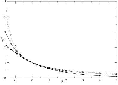
Figure 1: Analytical calculation of equation (52) for $\kappa_{e}^{(p)}$ for $a=0$ in 2(solid line), 3 (dashed line) and 4 (dotted line) dimensions, confronted with direct simulation of the random diffusivity problem. The simulation results are shown as circles ( $2D$), squares ($3D$) and stars for (4D). We have excellent agreement except at negative $\beta$ except for $\beta<-1$ in $4D$. This is to be expected as locally $\kappa({\mathbf{x})}$ can become very big which is obviously a problem for simulation.

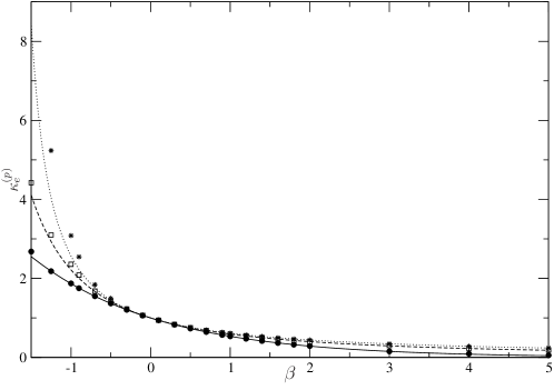
Figure 2: Analytical calculation of equation (52) for $\kappa_{e}^{(p)}$ for $a=0.5$ in 2 (solid line), 3 (dashed line) and 4 (dotted line) dimension, confronted with direct simulation of the random diffusivity problem. The circles stand for $2D$, squares for $3D$ and stars for $4D$. We have an excellent agreement except for $\beta<-1$ in 4D. In this case, $\kappa_{e}^{(p)}$ become indeed very large which force us to use smaller time step and thus the simulations are harder.

The predictions of the RG analysis can also be directly compared with a simulation of the stochastic equation (1) and the results are found to be in excellent agreement for small values of $|\beta|$. However near the dynamical transition finite size effects play a role. Direct simulation of the gradient flow case also requires much longer simulation times to estimate the asymptotic diffusion constant as finite time corrections seem to be more importamt. It is clearly much better to simulate the stochastic equation (9) and then determine the effective diffusion constant for the gradient flow problem using the relation equation (11). The results using this method for the case $a=0$ are shown in figure (3). We see that the results for 3 and 4 dimensions are in excellent agreement with our analytical calculations and that for 2 dimensions the only discrepancy is at large positive values of $\beta$.

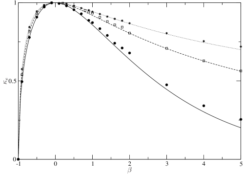
Figure 3: Renormalization group prediction for $\kappa_{e}$ for the case $a=0$ in 2 (solid line), 3 (dashed line) and 4 (dotted line) dimensions, confronted with numerical results deduced via the simulation of the random diffusivity problem and using equation (11) to estimate $\kappa_{e}$ ($2D$ circles, $3D$ squares and $4D$ stars). We see that the results are excellent and improve on increasing the spatial dimension.

5 Conclusion and Discussion

We have seen that the renormalization group scheme developed in [1] and [2] can be refined to take into account non-Gaussian potentials. The new scheme retains the merit of reproducing exactly known results in lower dimensions and has good agreement with numerical simulations in cases where exact results are not known. The main breakthrough is that this scheme is capable of predicting dynamical phase transitions where the self-diffusion constant vanishes, a transition analogous to the glass transition. A key point in the analysis was to apply the approximate renormalization group not to the problem of diffusion in a random gradient field but to a mathematically related problem of diffusion in a random diffusivity field. This renormalization group calculation applied to this problem produces a form of the celebrated Landau-Lifshitz-Matheron conjecture from the field of random porous media as given in equation (43).

Of course the problem we are considering is one with quenched disorder, in glass formers the disorder is thought to be somehow self induced. Let us consider for a moment the problem of $N$ Brownian particles (of bare diffusion constant 1) interacting via a pairwise potential $u$. The Langevin equation can be written as

$${d{\mathbf{X}}\over dt}={\mathbf{\eta}}-\beta\nabla\nu({\bf X})$$ (61)

Here the potential is given by

$$\nu({\bf X})=\sum_{i<j}u({\mathbf{X}}_{i}-{\mathbf{X}}_{j})$$ (62)

i.e. the energy due to the pairwise interaction between particles. The corresponding permeability problem thus has

$$\kappa({\mathbf{x}})=\exp(-\beta\nu({\mathbf{x}})).$$ (63)

Clearly the system is not disordered but we shall treat it as it were and apply the formula (43) to estimate the self diffusion constant. Firstly we have

$$\left\langle\kappa({\mathbf{x}})\right\rangle={N!\over V^{N}}Z_{N}$$ (64)

where $V$ is the volume of the system, $N$ the number of particles (assumed indiscernable) and $Z_{N}$ is the canonical partition function for the system. Here we have simply replaced the disorder average by the spatial average (this is in fact the correct average to make if one looks at the derivation of equation (11) [3, 7, 13] it is replaced by a disorder average by appealing to ergodicity). If one introduces the free energy per particle $f(\beta)$ we find that

$$\left\langle\kappa({\mathbf{x}})\right\rangle=\exp\left(-N(\beta f(\beta)-\ln(\rho)+1)\right),$$ (65)

where $\rho$ is the particle density $\rho=N/V$. Similarly we denote the dimension of the space of the diffusivity problem by $D=Nd$ where $d$ is the physical space dimension and find

$$\left\langle\kappa({\mathbf{x}})^{1-{2\over D}}\right\rangle^{1\over\left(1-{2\over D}\right)}=\exp\left[-N\left(\beta f\left(\beta\left(1-{2\over D}\right)\right)-{\ln(\rho)-1\over\left(1-{2\over D}\right)}\right)\right].$$ (66)

We see that the two quantities above have logarithms which are extensive in $N$ but we expect the self-diffusion constant to be intensive, remarkably the ratio of the two above quantities is intensive and we find to leading order in $N$ that

$$\kappa_{e}=\exp\left({2\beta^{2}\over d}f^{\prime}(\beta)+{2\ln(\rho)-2\over d}\right).$$ (67)

Now we use the trivial thermodynamic identity that the entropy per particle is given by $s=-\partial f/\partial T=\beta^{2}\partial f/\partial\beta$ and also the fact that at $\beta=0$ we have $s(0)=-\ln(\rho)+1$, to obtain

$$\kappa_{e} = \exp\left(2{(s(\beta)-s(0))\over d}\right)$$ (68)

$$= \exp\left({2\over d}s_{ex}(\beta)\right),$$

where $s_{ex}$ is simply the excess entropy per particle with respect to the perfect gas. Thus the approximative line of mathematical reasoning we have followed has lead to a quite interesting relation between a dynamic quantity (the diffusion constant) and a thermodynamic quantity (the excess entropy per particle). The celebrated Adam-Gibbs relation for glasses relates the relaxation time to the configurational entropy [22], here we have a relation between the self diffusion constant and the full entropy and the relationship is quite different from the Adam-Gibbs form. However for some time in the chemical physics literature [23, 24, 25, 26] it has been observed that the diffusion constant in molecular dynamics simulations, when written in dimensionless form, can often be well fitted (in the denser phase) by the expression

$$\kappa=C\exp(As_{ex}).$$ (69)

Now our computation is for Langevin systems so one would have to course grain a real molecular dynamics to a Brownian level to determine $\kappa_{0}$ (which here we have set to 1) for the effective Langevin dynamics; we thus cannot reasonably expect to predict the value $C$ without further study. However our naive prediction would be $A=2/d$. Numerical simulations [23] have revealed that $A$ varies quite weakly depending on the species, and it is reported that $A\approx 0.65$ for hard spheres and $A\approx 0.8$ for Lennard-Jones fluids, both in three dimensions. In another study it was proposed that $A=1$ [25] and the subject is still debated and studied (see [26]) for a recent review. Here we predict $A=2/3$ which is in intriguing agreement for the hard sphere result ! The only other analytical derivation that we are aware of for relations of the type of equation (68) is via mode coupling theory (and thus quite different to that given here) [27] where the effect of mixtures was also included. It will be interesting to see if this last application of our method could be refined to treat mixtures and also it should be confronted with numerical simulations of Langevin systems [28].

References

References

- [1] Dean DS, Drummond IT and Horgan RR 1994 J. Phys:A: Math Gen 27, 5135.
- [2] Deem MW and Chandler D 1994 J. Stat. Phys 76, 911.
- [3] Dean DS, Drummond IT and Horgan RR 2007 J. Stat. Mech. P07013.
- [4] Drummond IT, Horgan RR, and da Silva Santos CA 1998 J. Phys A: Math. Gen 31, 1341.
- [5] Touya C and Dean DS 2007 J. Phys. A: Math. Theor. 40, 919.
- [6] Dean DS , Drummond IT, and Horgan RR 2004 J. Phys:A: Math Gen 37, 2039.
- [7] Dean DS, Drummond IT, Horgan RR and Lefèvre A 2004 J. Phys. A : Math Gen 37, 10459.
- [8] Matheron G 1967 Eléments pour une theorie des milieux poreux, Paris; Masson.
- [9] King PR 1987 J. Math. Phys. 20, 3935.
- [10] Sposito G 2001 Transport Porous Med., 42,181.
- [11] D.T. Hristopulos 2003 Water Resour. 26, 279.
- [12] Eberhard J, Attinger S, and Wittum G 2004 Mutiscale Model. Sim. 2, 2259, 2004.
- [13] Dean DS, Drummond IT and Horgan RR 1997 J. Phys:A: Math Gen 30, 385.
- [14] Dykhne AM 1971 Sov. Phys.-JETP 32, 63.
- [15] Dykhne AM 1971 Sov. Phys.-JETP 32, 348.
- [16] De Wit. A 1995 Phys. Fluids 72, 553.
- [17] Kraichnan RH 1976 J. Fluid Mech. 77, 753.
- [18] Götze W 1989 Liquids, freezing and the glass transition Les Houches (North Holland, Amsterdam).
- [19] Vilgis TA 1993 Phys. Rev. B 47 2882.
- [20] Drummond IT, Hoch A and Horgan RR 1986 J. Phys:A: Math Gen 19, 387.
- [21] Honeycutt. RL 1992 Phys Rev A 45, 600.
- [22] Gutzow I and Schmelzer J 1995 The vitreous state Springer-Verlag (Berlin Heidelberg).
- [23] Rosenfeld Y 1977 Phys. Rev. A 15 2545.
- [24] Rosenfeld Y 1999 J. Phys. Condens. Matter 11 5415.
- [25] Dzugutov M 1996 Nature 381 137.
- [26] Mittal J, Errington JR and Truskett M 2007 J. Phys. Chem. B 111, 10054.
- [27] Samanta A, Musharaf Aki Sk and Ghosh SW 2001 Phys. Rev. Lett. 87 245901.
- [28] Dean DS and Touya C, work in progress.