3D hydrodynamical simulations of the large scale structure of W50-SS433

Abstract

We present 3D hydrodynamical simulations of a precessing jet propagating inside a supernova remnant (SNR) shell, particularly applied to the W50-SS433 system in a search for the origin of its peculiar elongated morphology. Several runs were carried out with different values for the mass loss rate of the jet, the initial radius of the SNR, and the opening angle of the precession cone. We found that our models successfully reproduce the scale and morphology of W50 when the opening angle of the jets is set to 10$\degr$ or if this angle linearly varies with time. For these models, more realistic runs were made considering that the remnant is expanding into an interstellar medium (ISM) with an exponential density profile (as HI observations suggest). Taking into account all these ingredients, the large scale morphology of the W50-SS 433 system, including the asymmetry between the lobes (formed by the jet-SNR interaction), is well reproduced.

1 Introduction

The standard supernova remnant (SNR) evolution theory, proposed by Woltjer (1970, 1972), predicts a spherical morphology for remnants expanding into a uniform ISM. Observations show, however, that a spherical morphology is not the prevalent appearance of SNRs. Non-spherical morphologies can be produced by external or internal factors. Among the external factors are the existence of dense clouds or strong density gradients in the ISM where the SNR is expanding. Internally, in remnants resulting from a Type II SN explosion, a compact object (a neutron star or a pulsar for example) can remain inside the SNR, injecting enormous amounts of energy through its magnetic field and particle outflow, thus modifying the evolution of the host SNR.

Based on astronomical observations (mainly in radio continuum and X-ray), SNRs can be classified in three main morphological groups: (a) shell-type, when the remnant exhibits a shell morphology in both radio and X-ray images; (b) plerions or Crab-like type, when the morphology of the remnant resembles the appearance of a centre-filled nebula, similar to the Crab’s SNR (in this case the X-ray and radio emission mainly come from the central compact object and the SNR shell is not observed); and (c) composite, when the SNR has a shell-type morphology plus a central component. The thermal-composite or mixed SNRs belong to this group; they are characterised by a radio shell with thermal X-ray emission in the interior.

There are remnants with more complex morphologies that can be included in group (c); such is the case of W50 (Geldzahler et al., 1980; Downes, Pauls & Salter, 1986; Elston & Baum, 1987). The morphology of this remnant can be described as an almost spherical shell distorted by two symmetrical lobes along the East-West direction (see for example fig. 1a and 1b of Dubner et al. 1998). The source of relativistic jets SS433 (Abell & Margon, 1979; Fabian & Rees, 1979; Clark & Murdin, 1978; Hjellming & Johnston, 1982; Margon, 1984; Hjellming & Johnston, 1985) is located at the centre of W50. These jets have a speed of 0.26c and a precession period of 164 days and form a cone around the source with a half-angle of $\sim$20^∘. Analysis of the nature of the system reveals that the source of SS433 is a binary system, with an orbital period of 13 days; the jets’ axis has an additional nodding motion with a period of 6 days (Newsom & Collins 1981, see also Collins & Scher 2002). The precession axis is aligned with the east-west direction of the W50 lobes. Several authors have given different explanations for this alignment. These explanations can be grouped in two possible scenarios: first, the SS433-W50 system is formed by the interaction of the jets of SS433 with the ISM (homogeneous or previously swept up by the stellar wind of SS433), without being affected by the SNR (Königl, 1983; Begelman et al., 1980); second, the eastern and western lobes of the system were formed by the interaction of the jets with the SNR shell (Zealey, Dopita & Malin, 1980; Downes, Pauls & Salter, 1986; Murata & Shibazaki, 1996). Observationally, Elston & Baum (1987) found evidence supporting the latter idea. Later on, Dubner et al. (1998) also found evidence based on high resolution radio-continuum images obtained with the Very Large Array (VLA). This was recently confirmed by the X-ray XMM-Newton observations of Brinkmann et al. (2007).

A recent work carried out by Durouchoux et al. (2001) (and references therein) examines SNR catalogs looking for other possible examples of SNRs with a similar elongated appearance. They identify three possible candidates: G309.2-00.6, G41.1-0.3 located in the 3C397 complex, and G54.1+0.3.

Following the jet-SNR interaction scenario, Velázquez & Raga (2000) carried out 2D axisymmetric numerical simulations to describe the W50-SS433 system, obtaining a rough agreement between their model and observations. Their model, however, was constrained by several hypothesis and assumptions.

In this work, we continue the study of Velázquez & Raga (2000), but remove several of their assumptions. We present 3D numerical simulations for the W50-SS433 system with the objective of providing a more realistic approach than the 2D model, following carefully the dynamics of the system as the precessing jets inject energy and momentum into the SNR cavity, collide with the SNR shock front, and change the spherical shape of the remnant. These simulations were carried out with the Yguazú-a code (, 2000; Raga et al., 2002).

The article is organised as follows. Section 2 gives the initial conditions of the numerical simulations and a brief description of the Yguazú-a code. The results are presented in Section 3. Finally, the discussion and conclusions of our work are given in Section 4.

2 Initial conditions and the Yguazú-a code

Table 1: Parameters for the numerical simulations. lin means $\alpha(t)=\omega_{1}t$, see text for details.

Model	M1	M2	M3	M4	M5
$\dot{M}_{j}(10^{-6}M_{\odot}yr^{-1})$	5	100	5	5	5
$\alpha$	20	20	20	10	20(lin)
$R_{SNR}(pc)$	20	20	10	20	20

As input data, we will use known values of the initial SN energy explosion, jet velocity, density, precession period and angle, etc., based on the only well-analysed observed case: the interaction between the relativistic jets from SS433 with the W50 SNR. Previous works have used 2D axisymmetric models of conical jets to describe this problem (Velázquez & Raga, 2000; Kochanek & Hawley, 1990), because the 164 day precession period of the jet (Margon et al., 1979; Hjellming & Johnston, 1988, 1985, 1982) is considerably shorter than its dynamical evolution time, defined as $t_{dyn}=R_{l}/v_{j}\simeq 140$ yr. Nevertheless, several assumptions on the geometry of the jet are needed in this type of model. 2D axisymmetric simulations model the symmetry axis as a reflecting boundary. This condition can produce undesirable effects such as an increase of the momentum flow along the symmetry axis (see for example Raga et al., 2007). Furthermore, in 2D axisymmetric simulations, it is not clear if the precession cone should be modelled by a filled conical jet or a hollow conical jet to represent the actual physical processes that take place in such a system. With a full 3D simulation, the assumption of axisymmetry is no longer needed and problems regarding the reflection condition disappear.

We have carried out numerical simulations of five models for precessing jets evolving into a SNR cavity. The main parameters for these models (the half-angle of precession $\alpha$, the initial SNR radius $R_{SNR}$ and the jet’s mass injection rate $\dot{M}_{j}$) appear in table 1.

The numerical simulations were made employing the 3D version of the Yguazú-a code (see (2000) and Raga et al. (2002)). The main characteristic of the code is that it has an adaptive grid and integrates the gas-dynamical equations with a second order accuracy (in space and time) implementation of the “flux-vector splitting” algorithm of van Leer (1982). Together with the gas-dynamical equations, a system of rate equations for atomic/ionic species is also calculated, which are then used to compute a non-equilibrium cooling function (a parameterised cooling rate being applied for the high temperature regime). They are also integrated with the gas-dynamical equations. Rate equations for H I-II, He I-III, C II-IV, and O I-IV are considered (for more details about reaction and cooling rates see Raga et al. 2002).

In all simulations, a 5-level binary adaptive grid was used with a maximum resolution of $4.8\times 10^{17}$ cm. A Cartesian computational domain of $512^{3}$ pixels with a size of 80 pc along each axis was employed. The centre of the SNR and the source of the jets is located at the centre of the $xy-$ plane with $z=0$. Free outflow conditions were employed on each computational domain boundary.

The initial conditions for all models were adopted from different multiwavelength observational studies. For the jet, we adopt velocity $v_{j}=7.5\times 10^{9}{\rm cm\ s^{-1}}$, temperature, $T_{j}=1\times 10^{7}{\rm K}$, radius, $2.4\times 10^{18}{\rm cm}$ (equivalent to 5 pixels for the maximum resolution) and length, $4.8\times 10^{18}{\rm cm}$. For the ISM we adopt density, $0.01{\rm cm^{-3}}$ (Safi-Harb & Oegelman, 1997), temperature, $1\times 10^{4}{\rm K}$ and velocity equal to zero; finally, the SNR was initialised employing the autosimilar Sedov solution (Sedov, 1959) considering a remnant radius of $6.2\times 10^{19}$ cm or 20 pc (except for the model M3 that has half of this radius) and a SN explosion energy of $5\times 10^{50}$ ergs.

2.1 The ISM density gradient

It is known that the system W50-SS433 is embedded in an ISM with a strong density gradient (Dubner et al., 1998), unlike the constant density ISM we have assumed so far. Thus, we made other runs of models M4 and M5 including a stratified ISM. In this case the Sedov solution is not valid, so we divide the simulation in two parts. In the first one, the SN explosion is simulated considering that an initial energy of $5\times 10^{50}\ \mathrm{ergs}$ (the same energy used in the previous models) is put into a sphere with a radius of 1.5 pc and a mass of 3 $M_{\odot}$, uniformly distributed within this radius. Actually, the details of the SN explosion are not important if our interest is to study an evolved SNR, such as W50, because when the remnant enters into the adiabatic or Sedov evolution phase, the SNR has already lost the memory of the initial conditions. The only important parameter is the initial explosion energy $E_{0}$. The SNR evolution is followed until the remnant shell reaches a radius of $\simeq 21$ pc, at an integration time of $t=6000$ yr. In the second part, the jets are “turned on” within the obtained SNR shell using the same parameters as in the previous models.

For these new runs, a computational domain of $512\times 512\times 1024$ pixels was used, corresponding to a physical size of $80\times 80\times 160$pc. Both SNR and source jets were located at the centre of the computational domain. Free outflow conditions were applied on each grid boundary.

The density stratification is given by $\rho(x,z)=\rho_{0}$ exp$(-z_{p}/h_{z})$, where $z_{p}=x~{}\textrm{sin}\beta-z~{}\textrm{cos}\beta$, $h_{z}=20$pc is a characteristic scale length, and $\beta=20\degr$ is the inclination of the precession cone axis with respect to the $z-$ axis.

3 Results

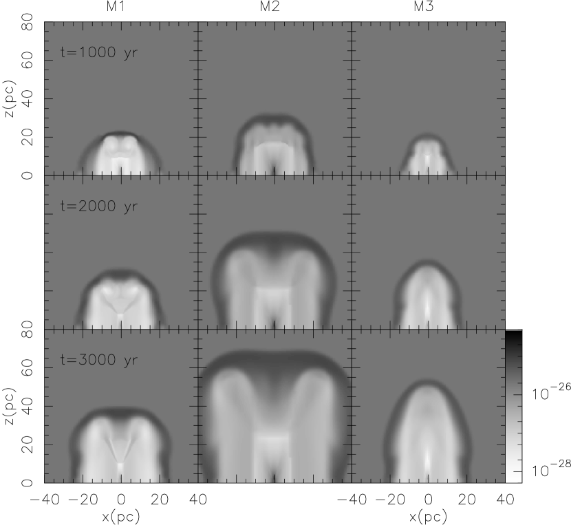
Figure 1: Comparison of the temporal evolution of density stratification maps for models M1, M2 and M3 (left to right). The grey scale is logarithmic and the density is given in units of $gr\ cm^{-3}$.

As a first analysis, we study the interaction of the precessing jets with the shell of the SNR for $\alpha=20^{\circ}$. With the objective of reproducing the observed morphology of W50, we explore different values for the jet’s mass injection rate (models M1 and M2) and the SNR radius (models M1 and M3). The range used for $\dot{M}_{j}$ lies in the range inferred from X-ray observations (Safi-Harb & Oegelman, 1997; Kotani et al., 2006). The time delay between the SN explosion and the “turn on” of the jets is not well-known; this motivated us to make a run with a shorter SNR radius to simulate a shorter time delay (model M3).

Figure 1 shows the temporal evolution of the density distribution for these models. The maps were obtained making a cut in the $xz-$ plane passing through the centre of the jet’s source. Kochanek & Hawley (1990) reported that hollow conical jets, expanding into a uniform ISM, experience a geometrical dilution of the momentum flux which prevents the jet’s expansion. A similar situation occurs in models M1-M3. Even though we are not using the hollow conical jet approximation, we expect that the symmetric approximation will be valid for distances sufficiently close to the source. The asymmetry in the density distribution due to the jet’s precession can be appreciated by zooming on the central region; this is shown in fig. 2 for model M1. The left and right panels display the $xz-$ and $yz-$ density distributions, respectively. The bottom panel is the point to point ratio between these two projections, and it clearly shows the asymmetry of the system, being larger for larger distances to the source. Even when the axial asymmetries are not very large, the figure shows the advantage of a 3D simulation over the usual assumption of axial symmetry.

Comparing models M1 and M2, it is clear that the increase of $\dot{M}_{j}$ does not change the general structure of the cavity shell; the main difference is the larger cavity size for model M2. In the case of model M3, with $R_{SNR}=10$ pc, the resulting morphology is very elongated along the jet axis, and the SNR shell quickly loses its identity.

In these models, the jet is moving into a stratified medium (the SNR cavity) which could bend the initial jet’s trajectory. However, a deflection of the jet is not observed. We conclude that a precessing jet with $\alpha=20^{\circ}$ moving into a remnant cavity cannot reproduce the observed shape of W50.

Because it was not possible to reproduce the morphology of $W50$ with models M1-M3, we ran a new simulation, model M4, with the same parameters as M1 but with $\alpha=10\degr$.

The left panels of figure 3 display the temporal evolution of the density stratification for model M4. By $t=1000$ yr, the SNR shell has been broken by the precessing jet. The evolution snapshots show that the jet has suffered a collimation process caused by the interaction of the jet’s bow shock and the SNR shell. As a result, secondary shocks are formed which further reflect themselves on the $z-$ axis. For $t=3000$ yr, we can see that there is a rupture of the primary lobe present at $t=2000$ yr. This pattern resembles the helical structure shown in the eastern lobe of W50. The result is also in agreement with the 2D axisymmetric modelling of Velázquez & Raga (2000).

3.1 The semi-aperture angle of the jets

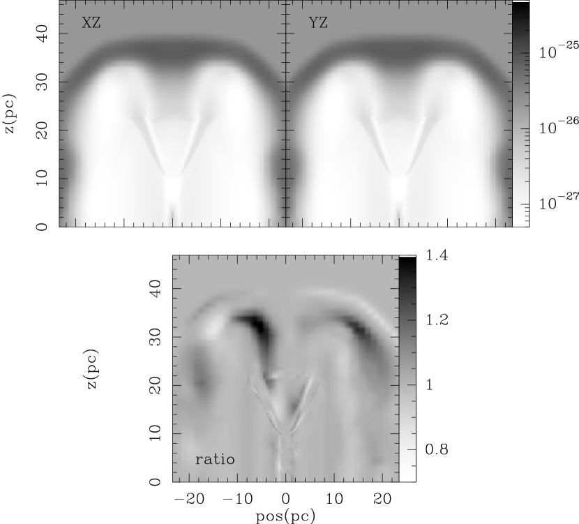
Figure 2: Asymmetry between xz and yz projections of the density distribution at $t=3000$ yr for model M1. Bottom panel displays the ratio between the $xz-$ and $yz-$ density distribution maps. If the system were perfectly symmetric, this ratio would be 1. Note that some regions show asymmetries with values $\sim$40% showing the importance of full 3D hydrodynamical simulations to model the system.

These results point to an apparent contradiction between the observed semi-aperture angle $\alpha$ and our numerical models. How can they be made compatible?. Previous X-ray observations (Watson et al., 1983; Brinkmann et al., 1996; Safi-Harb & Oegelman, 1997) have shown that the angle subtended by the “X-ray lobes” is smaller than expected from the precession cone of the innermost SS433 jets (40°). A possible solution is to consider that $\alpha$ is not constant during the jet evolution. We will use a model where $\alpha$ starts with a value equal to zero and then grows with time. We assume a simple model where $\alpha$ depends linearly on time: $\alpha=\alpha_{m}\omega t$ for $0\leq t\leq\tau_{c}$ and $\alpha=\alpha_{m}$ for $t>\tau_{c}$, where $\omega=1/\tau_{c}$, $\tau_{c}$ is a free parameter that was chosen to be 2000 yr in order to produce lobes with the desired size, and $\alpha_{m}=20\degr$ is the estimated value of the opening angle today (Abell & Margon, 1979).

This hypothesis is included in model M5 and the results are shown in the right panels of figure 3. The snapshots are for the same evolution times as the left panels. The shock front of the jet breaks the SNR shell as early as $t=1000$ yr and for $t=3000$ yr a well-formed lobe is observed. Unlike model M4, there is no secondary breaking of the lobe.

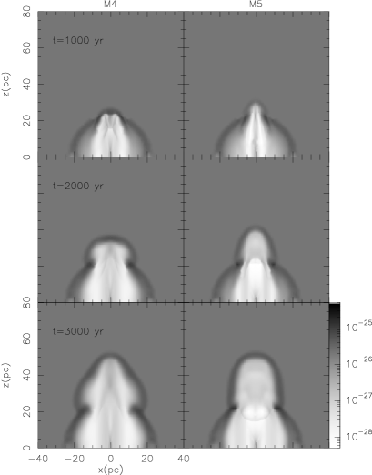
Figure 3: Snapshots of the density distribution for models M4 (left panel) and M5 (right panel) at integration times $1000$ yr, $2000$ yr and $3000$ yr. Note that the spherical symmetry of the SNR is broken by the precessing jet and the formation of the lobe is clearly observed.

3.2 The ISM density gradient effect

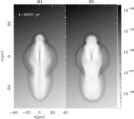
Figure 4: The same parameters for the jet and SNR as for models M4 (left panel) and M5 (right panel) but the ISM has a density gradient increasing along an axis tilted by an angle of $20\degr$ with respect to the vertical axis. The snapshot is for $t=3600$ yr after the jet is turned on (a total evolution time of 9600 yr).

The effects from the inclusion of the ISM density gradient to our model, described in subsection 2.1, can be seen in figure 4. The left panel shows the density distribution on the $xz$ plane for a run with the same parameters as for model M4, while the right panel has the same parameters as model M5. These maps were obtained for an integration time of 3600 yr after the jet is turned on (corresponding to a total evolution time of 9600 yr). The ISM density gradient produces an extra asymmetry in the system which is clearly seen by the difference in the evolution of the lobes corresponding to the upper (western) and lower (eastern) jets. In the region where the ISM density is higher, the effect is to slow the SNR shell evolution and also to slow the penetration of the SNR shell by the jet’s cocoon.

In order to have a more direct comparison with the actual observed system, we produced maps of the electronic density integrated along the line of sight for the new runs of models M4 and M5. These maps are shown in the left and right panels of figure 5, respectively. An inclination angle of $21\degr$ with respect to the plane of the sky has been taken into account. The angle was chosen according to the observed value given by Hjellming & Johnston (1988). The electronic density is a measure of the ionised zones in the system, it is expected that it will be enhanced just behind the shock fronts. For this reason, the electronic density is a good tracer of the structure observed in radio-continuum images. The physical sizes of the resulting distorted SNR shell are $56\mathrm{pc}$ and $103\mathrm{pc}$, along the $x-$ and $z-$ directions, respectively. These physical sizes correspond to angular sizes of $1\degr 4\arcmin\times 1\degr 58\arcmin$ (if a distance of 3 kpc to SS433 is assumed), which are very similar to the observed dimensions ($1\degr\times 2\degr$). The main difference between the panels of figures 4 and 5 is that the more evolved lobe (lower) is more collimated for the case of model M4 than for M5.

Figure 6 illustrates the comparison between simulations (left panel of fig. 5) and radio observations. The similarity with the system W50-SS433 is appealing. The eastern (left) lobe in the simulation is however wider than the observed one. A possible cause for this difference is the presence of an HI cloud in the southern part of the eastern lobe (as suggested by Dubner et al., 1998), which could have contributed to an extra collimation of the lobe. Since this cloud is not included in our models, the result is a wider lobe. It is important to point out that an ideal comparison would be with synthetic radio maps generated directly from the simulations. However, our models do not include magnetic fields and thus it is not possible to produce such maps.

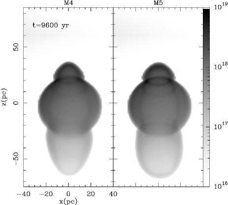
Figure 5: Electronic density integrated along the line of sight with a $21\degr$ inclination angle with respect to the plane of the sky for the same models as figure 4. The grey scale is logarithmic and is given in units of $\mathrm{cm}^{-2}$

4 Summary and Conclusions

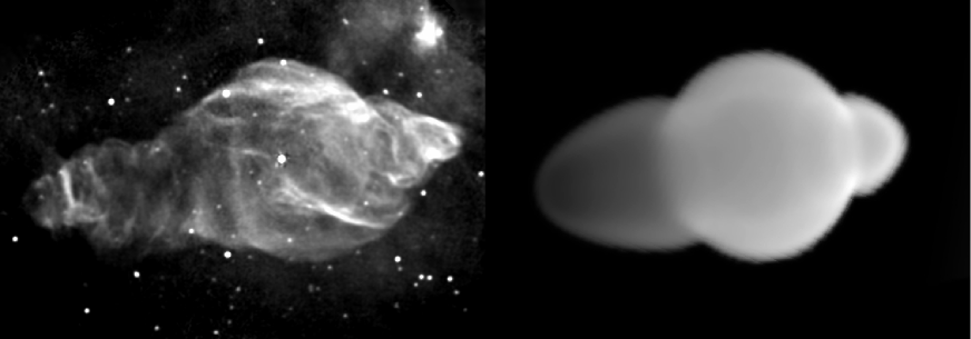
Figure 6: Comparison of the radio-continuum image with the simulated column electronic density map of model M4. The left panel shows the 1415 MHz image in grey scale and contours of the W50 SNR, obtained with the VLA by Dubner et al. (1998), in equatorial coordinates (North is up). The right panel shows the simulated map in a grey color scale. A distance of 3kpc to SS433 was assumed.

We have analysed the interaction between a precessing jet and a SNR shell using a 3D hydrodynamical simulation with the goal of studying the large scale structure of the SS433-W50 system. The motivation for doing so is to put aside one of the usual assumptions made in the past regarding this kind of system, namely, using a cone (hollow or filled) as an approximation to model the jets from the source SS433. The precession period of the jets is lower than the dynamical time of the system, therefore, it would be expected that the precessing jets can be modelled by a single axially symmetric conical jet. Nevertheless, analysing our simulations, we found that there is a significant axial asymmetry, especially for material located far away from the central source ($\sim 20-40\%$ of the ratio between the $xz$ and $yz$ density projections, see fig. 2). These results confirm the advantages of using 3D over 2D axisymmetric simulations.

We found that the simple simulated model with a constant value for the aperture angle, as reported observationally for the jets in SS433: $\alpha=20\degr$, fails to reproduce the observed morphology of this system. This result holds in spite of exploring a large range of values for the mass loss rate and the initial radius of the SNR (models M1-M3, see fig. 1). This radius is connected with the time delay between the SN explosion and the “turn on” of the jets. If this delay is too short, the jet’s cocoon sweeps up the SNR shell erasing all traces of the initial spherical morphology (model M3, right panel fig. 1).

If the value of $\alpha$ is arbitrarily reduced by half (model M4, see left panel of fig. 3), then the shock front of the jets is collimated enough to break the SNR shell, forming two lobes very similar to those observed. This result is related to the observational fact that at a distance of $\sim 6\times 10^{19}$cm from the source center, the angular extent of the X-ray jet is $\sim 18\degr$ (see for instance, Brinkmann et al., 2007), far below the expected $40\degr$ of the original model. This suggests a re-collimation mechanism that is still unknown. It is no surprise then that the large scale morphology of the system is reproduced well by our model when the opening angle is artificially reduced by half.

Such results led us to explore a different model where the value of $\alpha$ changes with time (model M5, see right panel of fig. 3), starting from zero and growing linearly until it reaches the constant value of $\alpha=20\degr$. This model also successfully reproduces the expected morphology. It is interesting to note that the corkscrew patterns observed in radio maps, at the tips of both Eastern and Western lobes of W50 (possibly produced by precession of the arcsecond-scale jet from SS 433) are limited spatially by a cone which seems to be smaller than the derived $\sim 20^{\circ}$ half-opening angle of the sub-arcsecond-scale jet. This is clearly illustrated in figure 1 of Moldowan et al. (2005), where a $\sim 20^{\circ}$ half-opening cone is superimposed on the radio map of W50. The authors also suggest that the sub-arcsecond jet is playing a crucial role in determining the morphology of W50 nebula, since their Chandra observations of the inner region of the west lobe of W50 show a good correlation between the precession of the jet and the X-ray emission. Based on this evidence, we presented here a numerical exercise, in order to investigate the morphological effects of a time varying opening angle jet on the whole structure of the nebula.

Finally, in order to give a more realistic model, two more simulations were made by using the parameters of models M4 and M5 but taking into account the observed density gradient of the ISM surrounding W50 (Dubner et al., 1998). In these runs the Sedov solution for the SNR was not used, instead, the simulations were divided in two stages: in the first one the SNR evolves alone; the second part follows with the turn on of the jets. The effect of the ISM density gradient is to produce different evolutionary patterns for the two lobes, making one of them more developed (see fig. 4). Given the fact that in our description the magnetic field is not included, it is not possible to generate synthetic radio continuum maps; an alternative was to present maps of the electronic density integrated along the line of sight, which is a good tracer of the shock fronts. An inclination of the system with respect to the plane of the sky of $\sim 21\degr$ was considered to obtain this map (see fig. 5).

In regard to the scale of the system, our models give physical sizes of $56\mathrm{pc}\times 103\mathrm{pc}$, which are similar to the observed dimensions, if a distance of 3 kpc is considered for W50 (based on the HI study of Dubner et al., 1998). There are other distance estimations for this remnant in the literature. Recently, Lockman et al. (2007) gives a distance between 5.5 and 6.5 kpc. This however does not change our main results, it would only be necessary to re-scale the simulated sizes and times.

In summary, the presented 3D models of the precessing jets of SS433 interacting with the shell of W50 reproduce the global characteristics (morphology and size) of this astrophysical object (see fig. 6), giving a closer qualitative and quantitative agreement with observations. It is however important to say that the model is still far from being complete; it is of key importance to propose and test a model that can account for the early re-collimation of the jets. The magnetic field could be included in future works as a possible solution to this problem (this was analytically treated by Kochanek 1991, but for conical jets moving into an uniform ISM). Other details of the structure of the system, such as the reported bend in the eastern jet’s propagation direction (see for example Brinkmann et al. (2007)) can be studied by simulating a more complex ISM. Also, future works could focus on the late evolution of the jets, when they are far from the central regime.

References

- Abell & Margon (1979) Abell, G. O., & Margon, B. 1979, Nature, 279, 701
- Begelman et al. (1980) Begelman, M. C., Hatchett, S.P., McKee, C. F., Sarazin, C. L., & Arons, J. 1980, ApJ, 238, 722
- Brinkmann et al. (1996) Brinkmann, W., Aschenbach, B., & Kawai, N. 1996, A& A, 312, 306
- Brinkmann et al. (2007) Brinkmann, W., Pratt, G. W., Rohr, S., Kawai, N., & Burwitz, V. 2007, A& A, 463, 611
- Clark & Murdin (1978) Clark, D. H., & Murdin, P. 1978, Nature, 276, 44
- Collins & Scher (2002) Collins, G. W., & Scher, R. W. 2002, MNRAS, 336, 1011
- Downes, Pauls & Salter (1986) Downes, A. J. B., Pauls, T., Salter, C. J. 1986, MNRAS, 218, 393
- Dubner et al. (1998) Dubner, G. M., Holdaway, M., Goss, W. M., Mirabel, I. F., 1998, AJ, 116, 1842.
- Durouchoux et al. (2001) Durouchoux, P., Sood, R., Safi-Harb, S., Lu, F. J., O’Neill, P., Flohic, H., & Lefevre, F. 2001, Astrophysics and Space Science Supplement, 276, 139.
- Elston & Baum (1987) Elston, R., & Baum, S. 1987, AJ, 94, 1633
- Fabian & Rees (1979) Fabian, A. C., & Rees, M. J. 1979, MNRAS, 187, 13
- Geldzahler et al. (1980) Geldzahler, B. J., Pauls, T., & Salter, C. J. 1980, A& A, 84, 237
- Hjellming & Johnston (1982) Hjellming, R. & Johnston, K. 1982, in IAU Symposium 97, Extragalactic Radio Source, Ed.: D. Heeschen & C. M. Wade (Dordrecht: Reidel), p.97.
- Hjellming & Johnston (1985) Hjellming, R. & Johnston, K. 1985, in Radio stars, Ed.: R. M. Hjellming & D. M. Gibson (Dordrecht: Reidel), p. 309.
- Hjellming & Johnston (1988) Hjellming,R. M., & Johnston, K. J. 1988, ApJ, 328, 600
- Kochanek & Hawley (1990) Kochanek, C. S. and Hawley, J. F. 1990, ApJ, 350, 561.
- Kochanek (1991) Kochanek, C. S. 1991, ApJ, 371, 289
- Königl (1983) Königl, A. 1983, MNRAS, 205, 471
- Kotani et al. (2006) Kotani, T., Trushkin, S. A., Valiullin, R., Kinugasa, K., Safi-Harb, S., Kawai, N., & Namiki, M. 2006, ApJ, 637, 486
- Lockman et al. (2007) Lockman, F. J., Blundell, K. M., & Goss, W. M. 2007, MNRAS, 381, 881
- Margon et al. (1979) Margon, B., Grandi, S. A., Stone, R. P. S., & Ford, H. C. 1979, ApJ Lett., 233, L63
- Margon (1984) Margon, B. 1984, ARA& A, 22, 507
- Moldowan et al. (2005) Moldowan, A., Safi-Harb, S., Fuchs, Y. & Dubner, G. 2005, Advance in Space Research, 35, 1062
- Murata & Shibazaki (1996) Murata, K. & Shibazaki, N. 1996, PASJ, 48, 819
- Newsom & Collins (1981) Newsom, G. H., & Collins, G. W., II 1981, AJ, 86, 1250
- (26) Raga, A. C., Navarro-González, R., Villagrán-Muniz, M., 2000, RMxAA, 36, 67. AdSpR, 35, 1027
- Raga et al. (2002) Raga, A. C., de Gouveia Dal Pino, E. M., Noriega-Crespo, A., Mininni, P. D., & Velázquez, P. F. 2002, A& A, 392, 267
- Raga et al. (2007) Raga, A. C., Esquivel, A., Riera, A., & Velázquez, P. F. 2007, ApJ, 668, 310
- Safi-Harb & Oegelman (1997) Safi-Harb, S., & Oegelman, H. 1997, ApJ, 483, 868
- Sedov (1959) Sedov, L. I. 1959, Similarity and Dimensional Methods in Mechanics, New York: Academic Press, 1959,
- van Leer (1982) van Leer, B. 1982, Numerical Methods in Fluid Dynamics, 170, 507
- Velázquez & Raga (2000) Velázquez, P.F., Raga, A. C., 2000, A& A, 362, 780
- Verbunt (1993) Verbunt, F. 1993, ARA& A, 31, 93
- Watson et al. (1983) Watson, M. G., Willingale, R., Grindlay, J. E., & Seward, F. D. 1983, ApJ, 273, 688
- Woltjer (1970) Woltjer, L., 1970, IAU Symp., 39, 229.
- Woltjer (1972) Woltjer, L., 1972, ARA& A, 10, 129.
- Zealey, Dopita & Malin (1980) Zealey, W. J., Dopita, M. A. & Malin, D. F. 1990, MNRAS, 192, 731