Fingerprint for Network Topologies

Abstract

A network’s topology information can be given as an adjacency matrix. The bitmap of sorted adjacency matrix (BOSAM) is a network visualisation tool which can emphasise different network structures by just looking at reordered adjacent matrixes. A BOSAM picture resembles the shape of a flower and is characterised by a series of ‘leaves’. Here we show and mathematically prove that for most networks, there is a self-similar relation between the envelope of the BOSAM leaves. This self-similar property allows us to use a single envelope to predict all other envelopes and therefore reconstruct the outline of a network’s BOSAM picture. We analogise the BOSAM envelope to human’s fingerprint as they share a number of common features, e.g. both are simple, easy to obtain, and strongly characteristic encoding essential information for identification.

1 Introduction

During the last decade there has been an international effort to understand the structure and dynamics of complex networks in social, biological, and technology systems wasserman94 ; watts99 ; Barabasi99 ; strogatz01 ; albert02 ; Maslov02a ; bornholdt02 ; newman03a ; dorogovtsev03a ; Pastor04 ; boccalettia06 ; newman06 . These networks are very large, containing thousands or even millions of entities (nodes) interacting with each other (links), and their structures are irregular, evolving and inherently stochastic. The statistical physics methods have been widely used in studying complex networks.

Complementary to this effort, a number of network visualisation tools have been proposed to illustrate network topologies, such as alvarez05 ; Guo07a ; Chakrabarti07 . These techniques take the advantage of human being’s extraordinary ability in recognising patterns in images and therefore allow us to compare two networks by seeing whether the networks visualisations look similar to each other.

Of our particular interest is a tool called the bitmap of sorted adjacency matrix (BOSAM) Guo07a . It sorts a network’s nodes in a specific order such that the bitmap representation of the reordered adjacency matrix resembles a ‘flower’. The shape of the flower reveals many topological properties of the network. A BOSAM flower consists of a series of ‘leaves’, each of which is characterised by its envelope.

In this paper we demonstrate and mathematically prove that the way the adjacency matrix is reordered for BOSAM gives rise to a self-similar relation between the envelopes of the leaves. This self-similar property allows us to use just one envelope to predict all other envelopes and therefore recover the shape of a BOSAM flower. We also show that if a network preserves its macroscopic structure during the network growth, the BOSAM envelopes scale with the network’s size. We remark that an envelope of a network’s BOSAM is analogous to a fingerprint of a human being, which is a small token, easy to obtain, valid for life, and encodes essential information for identification.

2 Bitmap Of Sorted Adjacency Matrix

For a network with $N$ nodes, the connectivity information between the nodes can be given as an $N*N$ adjacency matrix, in which entry $a_{ij}$ is the number of links connecting between nodes with indexes $i,j\in\{1,2,...,N\}$. For an undirected, simple network (no self-loop or repeat link), the adjacency matrix becomes a symmetric $(0,1)$-matrix with zeros on its diagonal, where entry $a_{ij}$ is mirrored by entry $a_{ji}$. This matrix can be represented as a black-and-white bitmap, i.e. if $a_{ij}=1$, a black pixel is placed at the coordinate of $(i,j)$; otherwise a white pixel is placed there. One can see such a bitmap is not very helpful if node indexes are randomly assigned.

Degree $k$ is defined as the number of links a node has. For a given network, we sort nodes in ascending order of the degree. For nodes having the same degree, we arrange them in ascending order of the largest neighbor degree, $\omega$, which is the largest degree of a node’s neighbours. For nodes having both the same degree and the same largest neighbor degree, we reorder them in ascending order of the largest neighbor index, $e$, which is the largest index of a node’s neighbours. We then reassign each node a new index using the node’s position in the sorted list. Then, for two nodes with indexes $i<j$, we have one of the followings:

• $k_{i}<k_{j}$;

• $k_{i}=k_{j}$ and $\omega_{i}<\omega_{j}$;

• $k_{i}=k_{j}$, $\omega_{i}=\omega_{j}$ and $e_{i}<e_{j}$.

The above node sorting rule produces a reordered adjacency matrix, whose bitmap visualisation is called the bitmap of sorted adjacency matrix (BOSAM). Fig. 1 shows BOSAMs for six networks. The names and sources of the datasets for these networks are given in Table 1. Each BOSAM picture resembles a ‘flower’ which consists of a series of ‘leaves’ symmetrically arranged along the bitmap’s diagonal. The shape of the flower reflects a number of network topological properties. For simplicity, in the following we only discuss vertical leaves above the diagonal.

Table 1: Properties of networks under study: (a) the Erdös-Rényi (ER) model erdos59 which generates random networks having a Poisson degree distribution; (b) the Barabási-Albert (BA) model Barabasi99 which generates scale-free networks with a power-law degree distribution; (c) the Positive-Feedback Preference (PFP) model zhou04d ; zhou06b ; zhou07a which generates Internet-like networks; (d) the scientific collaboration network newman01a ; newman01b , in which nodes represent scientists and a connection exists if they coauthored at least one paper in the e-print archive http://xxx.lanl.gov/archive/cond-mat/ from 1995 to 1998; (e) the protein interaction network Maslov02a ; colizza05 , in which nodes represent proteins in the yeast Saccharomyces cerevisiae (http://dip.doe-mbi.ucla.edu/) and a connection exists if they interact with each other; (f) the Internet network at the autonomous system (AS) level Pastor04 ; mahadevan05b based on the traceroute data collected by CAIDA in April 2003 itdk0403 ; CAIDA ; and (g, h) the Internet AS networks based on the BGP data collected by the Oregon Route Views project (http://www.routeviews.org/) in October 2001 and September 2006, respectively. On the AS Internet, nodes represent Internet service providers and a connection exists if they have a commercial agreement to exchange traffic. The shown properties are: the number of nodes $N$ and links $L$, the average node degree $\langle k\rangle=2L/N$, and the characteristic node degree $k^{*}$ which has the largest degree distribution.

	$N$	$L$	$\langle k\rangle$	$k^{*}$
(a) ER network	10,000	30,000	6	6
(b) BA network	10,000	30,000	6	3
(c) PFP network	10,000	30,000	6	2
(d) Scientific collaboration	15,179	43,011	5.7	2
(e) Protein interaction	4,713	14,846	6.3	1
(f) Internet (traceroute)	9,204	28,959	6.3	2
(g) Internet (BGP-2001)	12,033	21,742	3.6	1
(h) Internet (BGP-2006)	23,480	49,077	4.2	1

2.1 Degree distribution

The degree distribution $P(k)$ is the probability of finding a $k$-degree node in a network. For a network with $N$ nodes, the number of $k$-degree nodes is $N_{k}=N\cdot P(k)$, and the number of nodes with degrees equal to or smaller than $k$ as $N_{\leqslant k}=N\cdot\sum_{1}^{k}P(k)$. According to the node sorting rule of BOSAM, the indexes of $k$-degree nodes are $I_{k}=\{i\,|\,N_{\leqslant{k-1}}<i\leqslant N_{\leqslant k}\}$.

Each leaf is associated with a node degree $k$ because it is formed by pixels representing connections linking to $k$-degree nodes. In other words, the leaf for degree $k$ represents entries $\{a_{i,j}=1\,|\,i\in I_{k}\}$ in the reordered adjacency matrix. Thus the width of the $k$-degree leaf is $N_{k}$.

In Fig. 1, the widest leaf in the ER network’s BOSAM is for degree 6, which reflects that the network has a Poisson degree distribution which peaks at the average node degree of 6. Other networks are ‘scale-free’ having a power-law degree distribution Barabasi99 . This means most nodes are low-degree nodes, whereas a small number of nodes have very large degrees. This is reflected on BOSAMs as the width of leaves decreases rapidly with the node degree.

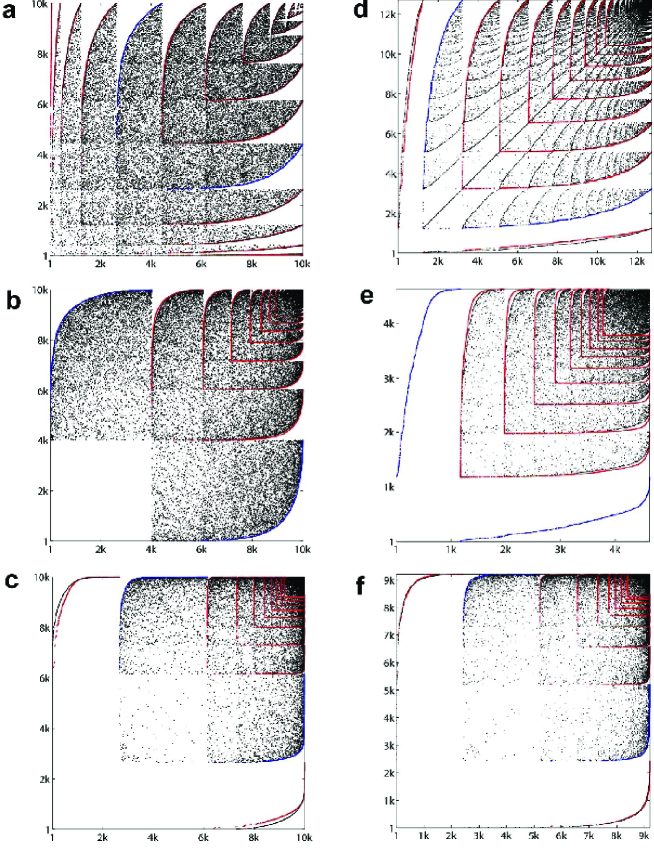
Figure 1: Bitmap of sorted adjacency matrix (BOSAM) for (a) the ER model, (b) the BA model, (c) the PFP model, (d) the scientific collaborations, (e) the protein interactions, and (f) the AS Internet. For each network, the envelope which is used as the root for the prediction is shown in blue colour and the predicted envelopes are shown in red colour.

2.2 Degree-degree correlation

Degree-degree correlation is a widely studied property vazquez03 ; Mahadevan06 . The protein interaction network, the Internet and the PFP network have a negative degree-degree correlation, or so-called disassortative mixing newman03 , which means low-degree nodes tend to connect with high-degree nodes and vice versa. This is reflected on their BOSAMs in Fig. 1 as pixels are densely distributed along the upper envelope of the leaves. In contrast, the scientific collaboration network exhibits a positive degree-degree correlation, or assortative mixing newman02 , which means nodes tend to connect with alike nodes of similar degrees. This is characterised on the BOSAM as a series of lines are radiated from the top-right corner across the leaves. The ER network and the BA network have a neutral degree-degree correlation, which is illustrated on the BOSAMs as pixels are fairly evenly distributed on the leaves.

2.3 Rich-club

In the Internet and the PFP model, the high-degree nodes, ‘rich’ nodes, are tightly interconnected with themselves, forming a rich-club Zhou04a ; zhou07b . This is reflected on their BOSAMs as the top-right corner is almost fully covered by pixels. This is not the case for the ER network and the BA network where high-degree nodes are sparsely interconnected with themselves.

In summary, BOSAM provides a simple and effective way to emphasising different network structures. We can compare network topologies by just looking at their BOSAMs. For example one can see that although the BA model has been widely used as a generic model for all scale-free networks, the model does not closely resemble the Internet, the protein interaction and the scientific collaborations. In fact the three real networks themselves are different from each other in profound ways. The PFP model well resembles the Internet based on the traceroute data (see Table 1).

3 Self-similar property of BOSAM

One improvement to the previous version of BOSAM Guo07a is that here we consider the largest neighbor index $e$ as well in the node sorting rule. This reduces zigzag in BOSAM and as a result the envelopes of the leaves become smooth, solid curves.

The envelope of the leaf for degree $k$ consists of $N_{k}$ pixels given as

$$E_{k}=\{(i,e_{i})|i\in I_{k}\},$$ (1)

where $e_{i}$ is the largest neighbor index of node $i$ and $I_{k}$ is the set of indexes of $k$-degree nodes. According to the node sorting rule of BOSAM (see Section 2), the degree of node $e_{i}$ is the largest neighbor degree of node $i$, i.e. $k_{e_{i}}=\omega_{i}$. One can see that the envelope $E_{k}$ is given by the cumulative distribution function $F_{k}(\omega)$, which is the probability for a $k$-degree node having the neighbours largest degree less than or equal to $\omega$.

3.1 Self-similar relation between BOSAM envelopes

Theorem 1. In a network, if a node’s neighbours degree $\mu$ is independent and identically distributed (i.i.d.), the cumulative distribution functions $F_{k}(\omega)$ and $F_{l}(\omega)$ for $k$-degree nodes and $l$-degree nodes, respectively, have the following self-similar relation,

$$F_{k}(\omega)=F_{l}(\omega)^{{}^{k}/_{l}}.$$ (2)

The proof of Theorem 1 is given in Appendix I. This self-similar property of BOSAM allows us to use just one envelope, we call it the root envelope, to predict all other envelopes (see the self-similar algorithm in Appendix III).

The characteristic degree $k^{*}$ is the node degree having the largest number of nodes, i.e. $N_{k^{*}}\geqslant N_{k}$ or $P(k^{*})\geqslant P(k)$. The envelope of the leaf for the characteristic degree contains more information than other envelopes. Fig. 1 illustrates the prediction result. For each network, we use the envelope for the characteristic degree (see Table 1) as the root envelope. We highlight the root envelope in blue colour and the predicted envelopes for other degrees in red colour. One can see that the predicted envelopes well overlap with the real envelopes beneath them.

3.2 Discussion

The self-similar relation between BOSAM envelopes is different from other scaling properties in networks, such as the scaling property of community size in social networks Guimera03 . As shown in the proof of Theorem 1, the self-similar relation between BOSAM envelopes is originated from the way we reorder the adjacency matrix, and therefore it is valid for all networks, regardless of networks degree distribution or degree-degree correlation.

The only condition for the proof of Theorem 1 is that the neighbours degree $\mu$ is independent and identically distributed (i.i.d.). One should not confuse this condition with the degree-degree correlation property of a network. The i.i.d. condition means that a network’s degree-degree correlation (whether the correlation is negative or positive) is consistent for all nodes. We can infer whether a network is i.i.d. by observing whether the prediction of BOSAM envelopes is accurate. Fig. 1 shows that most networks under study satisfy the i.i.d. condition. By comparison, the predicted envelopes for the protein interaction network do not precisely (but still quite closely) match the real envelopes. This suggest that the protein network are not strictly i.i.d..

3.3 Scaling of BOSAM envelopes

If two networks have the same macroscopic structure, their BOSAM pictures should look the same. This should be the case even if the networks are of different sizes. For example it is known that the BA model preserves its topological structure during network growth Barabasi99 . Therefore, as shown in Fig. 2-(a), the BOSAM pictures for the three BA networks with different sizes indeed look the same. We can use the scaling algorithm in Appendix IV to accurately predict the envelopes in the two larger networks (in red colour) from the envelopes in the small network (which themselves are predicted from the root envelope in blue colour). Thus the scaling property of BOSAM envelopes can be used to test whether two networks with different sizes have the same macroscopic structure.

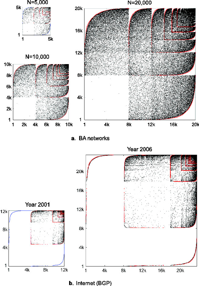
Figure 2: Prediction of BOSAM envelopes for growing networks. (a) BA networks with the number of nodes $N=5,000$, $N=10,000$ and $N=20,000$. (b) Internet networks based on BGP data collected in year 2001 and 2006 (see Table 1). In (a) and (b), red envelopes in larger networks are predicted from the blue envelope in the smallest network.

Fig. 2-(b) shows the BOSAM pictures for the Internet networks based on the BGP data collected in 2001 and 2006 (see Table 1). The envelopes in the large network are precisely predicted by scaling the envelopes in the small network. This suggests that during the 5-year period, although the Internet doubled its size, it well preserves its macroscopic structure.

4 BOSAM envelope as network fingerprint

Based on the above observations, we remark the analog between BOSAM envelope and human being’s fingerprint in the following ways. (1)  A BOSAM envelope is a small token of the network’s adjacency matrix, in the form of a set of coordinates $E_{k}=\{(i,e_{i})|i\in I_{k}\}$. Such a relatively small amount of information is easy to obtain, store and process. (2) A single BOSAM envelope is able to recover all other envelopes and thus provide an outline description of a network’s BOSAM. (3) The envelope fingerprint is valid for a growing network as far as the network preserves its macroscopic structure, just like a person’s fingerprint is valid for life. And (4) A BOSAM envelope contains essential information that characterises the network’s topology.

Fig. 3 shows one envelope fingerprint for each of the networks under study. For comparison purpose, all the envelopes shown are of the leaves for the node degree 2, except for the BA network which does not contain 2-degree nodes and therefore the envelope for degree 3 is shown instead. The size of the envelopes are normalised by the number of nodes in the networks. We can see the envelope fingerprint of the networks are strongly characteristic.

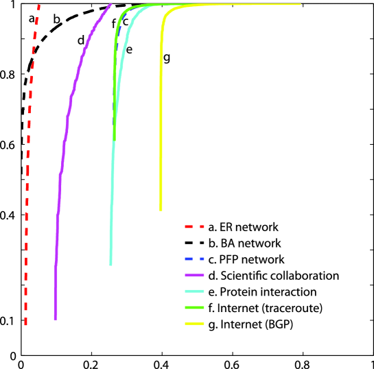
Figure 3: BOSAM fingerprint for all networks under study. Each envelope is normalised by the number of nodes in its own network.

Fig. 3 shows two fingerprints for Internet networks based on different data sources mahadevan05b . The fingerprint for the traceroute Internet (line 6) is positioned to the left of that for the BGP Internet (line 7). This reflects one of the key differences between the two data sources that 1-degree nodes count for a larger proportion in the BGP data than in the traceroute data. However the two fingerprints have the same shape, which suggests the fact that the macroscopic structure of the two Internet networks are similar. The close approximation between the traceroute Internet and the PFP network (line 3) is evidently shown by the close match of their fingerprints. One would expect that minor revision would enable the PFP model to resemble the BGP Internet as well.

5 Conclusion

BOSAM is a visualisation tool for network topologies. The simple tool provides an effective way to emphasise networks topological differences or similarities by just looking at the bitmap of reordered adjacency matrixes.

A network’s BOSAM is characterised by a series of leaves and the shape of the leaves are described by their envelopes. We show there is a self-similar relation between the envelopes for most networks. This properties allow us to use one single envelope to reconstruct all envelopes. For an evolving network which preserves its structure, the BOSAM envelopes scale with the growing size of the network. In these respects we suggest that the BOSAM envelope can be used as a self-similar fingerprint for network topologies.

Acknowledgments.

Y. Guo and C. Chen are supported by the Natural Science Foundation of China under grant no. 60672069 and 60772043, and the National Basic Research Program (973 Program) of China under grant no. 2007CB307101. S. Zhou is supported by the Royal Academy of Engineering and the UK Engineering and Physical Sciences Research Council (EPSRC) under grant no. 10216/70.

APPENDIX I   Proof of Theorem 1

For a $k$-degree node, the neighbours degree $\mu$ consists of $k$ variants $\mu_{1},\,\mu_{2},\,...,\,\mu_{k}\,$. We reorder them so that $\nu_{1}\leqslant\nu_{2}\leqslant...\leqslant\nu_{k}$. Thus the largest neighbor degree $\omega=\nu_{k}$.

According to the order statistic theory (see Appendix II ), the probability function of $\omega$ for $k$-degree nodes is given by

$$P_{k}(\omega)=P_{k}(\nu_{k})=k\,[F_{k}(\mu)]^{(k-1)}\,P_{k}(\mu)$$ (3)

where $P_{k}(\mu)$ is the probability function of $\mu$ and $F_{k}(\mu)$ is the cumulative distribution function of $\mu$, for $k$-degree nodes.

In a network where $\mu$ is i.i.d., we have $P_{k}(\mu)=P(\mu)$ and $F_{k}(\mu)=F(\mu)$. Then

$$P_{k}(\omega)=k\,[F(\mu)]^{(k-1)}\,P(\mu).$$ (4)

Therefore we have

$$F_{k}(\omega) = \int_{0}^{\omega}P_{k}(\omega)\,d\omega$$ (5)

$$= \int_{0}^{\mu}k\,[F(\mu)]^{(k-1)}\,P(\mu)\,d\mu$$ (6)

$$= \int_{0}^{\mu}k\,[F(\mu)]^{(k-1)}\,{dF(\mu)\over d\mu}\,d\mu$$ (7)

$$= \int_{0}^{F(\mu)}k\,[F(\mu)]^{(k-1)}\,d{F(\mu)}$$ (8)

$$= \int_{0}^{F(\mu)}\left([F(\mu)]^{k}\right)^{\prime}\,d{F(\mu)}$$ (9)

$$= [F(\mu)]^{k}.$$ (10)

Similarly we can have $F_{l}(\omega)=[F(\mu)]^{l}$ for $l$-degree nodes. Thus Theorem 1 is proved:

$$F_{k}(\omega)=[F(\mu)]^{k}=[~{}[F(\mu)]^{l}~{}]^{{}^{k}/_{l}}=[F_{l}(\omega)]^{{}^{k}/_{l}}.$$ (11)

APPENDIX II   Order statistic

Given a sample of $n$ variants $X_{1},X_{2}...,X_{N}$, reorder them so that $Y_{1}\leqslant Y_{2}\leqslant...\leqslant Y_{N}$. Then $Y_{r}$ is called the $r^{\,th}$ order statistic hogg70 for $r=1,2,...,N$.

If $X$ has the probability function $P(X)$ and the cumulative distribution function (CDF) $F(X)$, then the probability function of $Y_{r}$ is given by rose02

$$P(Y_{r})={N!\over(r-1)!\,(N-r)!}\,\,[F(X)]^{r-1}\,[1-F(X)]^{N-r}\,P(X).$$ (12)

Therefore the probability function of the largest value $Y_{N}$ is

$$P(Y_{N})=N\,[F(X)]^{N-1}\,P(X).$$ (13)

APPENDIX III   Algorithm for predicting envelopes for other degrees

For a network with $N$ nodes and degree distribution $P(k)$, if we know the BOSAM envelope $E_{l}=\{(i,\,e_{i})\,|\,i\in I_{l}\}$ for degree $l$, then we can use Theorem 1 to predict the envelope $E_{k}$ for degree $k$ as

$$\tilde{E_{k}}=\{(\tilde{i},e_{i})\,|\,i\in{I}_{l}\},$$ (14)

where

$$\tilde{i}=N_{<{k}}+N_{k}\left(\frac{i-N_{<{l}}}{N_{l}}\right)^{{}^{k}/_{l}}$$ (15)

and

$N_{k}=N\cdot P(k)$,   $N_{<k}=N\cdot\sum_{1}^{k-1}P(k)$.

APPENDIX IV   Algorithm for scaling envelopes with network size

For a network with $N$ nodes, if we know the BOSAM envelope $E_{k}=\{(i,\,e_{i})\,|\,i\in I_{k}\}$ for degree $k$, the scaling of the envelope to the network size of $N^{\prime}$ is given by

$$\tilde{E^{\prime}_{k}}=\{(\tilde{i^{\prime}},\tilde{e^{\prime}_{i}})\,|\,i\in{I}_{k}\},$$ (16)

where

$$\tilde{i^{\prime}}=i\,{N^{\prime}\over N}$$

and

$$\tilde{e^{\prime}_{i}}=e_{i}\,{N^{\prime}\over N}.$$

References

- (1) S. Wasserman and K. Faust, Social Network Analysis (Cambridge University Press, Cambridge, 1994).
- (2) J. Watts, Small Worlds: The Dynamics of Networks between Order and Randomness (Princeton Univeristy Press, New Jersey, USA, 1999).
- (3) A. Barabási and R. Albert, Science 286, 509 (1999).
- (4) S. H. Strogatz, Nature 410, 268 (2001).
- (5) R. Albert and A. L. Barabási, Rev. Mod. Phys. 74, 47 (2002).
- (6) S. Maslov and K. Sneppen, Science 296, 910 (2002).
- (7) S. Bornholdt and H. G. Schuster, Handbook of Graphs and Networks - From the Genome to the Internet (Wiley-VCH, Weinheim Germany, 2002).
- (8) M. Newman, SIAM Review 45, 167 (2003a).
- (9) S. N. Dorogovtsev and J. F. F. Mendes, Evolution of Networks - From Biological Nets to the Internet and WWW (Oxford University Press, Oxford, 2003).
- (10) R. Pastor-Satorras and A. Vespignani, Evolution and Structure of the Internet - A Statistical Physics Approach (Cambridge University Press, Cambridge, 2004).
- (11) S. Boccaletti, V. Latora, Y. Moreno, M. Chavez, and D.-U. Hwang, Physics Reports 424, 175 (2006).
- (12) M. Newman, A.-L. Barabási, and D. Watts, eds., The Structure and Dynamics of Networks (Princeton University Press, 2006).
- (13) J.-I. Alvarez-Hamelin, L. Dall’Asta, A. Barrat, and A. Vespignani, arXiv.org:cs/0504107.
- (14) Y. Guo, C. Chen, and S. Zhou, Electronics Letters 43, 597 (2007).
- (15) D. Chakrabarti, C. Faloutsos, and Y. P. Zhan, International Journal of Human-Computer Studies 65, 434 (2007).
- (16) A. Vázquez, M. Boguñá, Y. Moreno, R. Pastor-Satorras, and A. Vespignani, Phys. Rev. E 67 (2003).
- (17) P. Mahadevan, D. Krioukov, K. Fall, and A. Vahdat, in Proc. of SIGCOMM’06 (ACM Press, New York, 2006a), pp. 135–146.
- (18) M. E. J. Newman, Phys. Rev. E 67 (2003b).
- (19) M. E. J. Newman, Phys. Rev. Lett. 89 (2002).
- (20) S. Zhou and R. J. Mondragón, IEEE Comm. Lett. 8, 180 (2004a).
- (21) S. Zhou and R. Mondragón, New Journal of Physics 9, 1 (2007).
- (22) P. Mahadevan, D. Krioukov, M. Fomenkov, B. Huffaker, X. Dimitropoulos, K. Claffy, and A. Vahdat, Comput. Commun. Rev. 36, 17 (2006b).
- (23) R. V. Hogg and A. T. Craig, Introduction to Mathematical Statistics, 3rd ed. (New York: Macmillan, 1970).
- (24) C. Rose and M. D. Smith, Order Statistics (New York: Springer-Verlag, 2002).
- (25) P. Erdős and A. Rényi, Publ. Math. Debrecen 6, 290 (1959).
- (26) S. Zhou and R. J. Mondragón, Phys. Rev. E 70 (2004b).
- (27) S. Zhou, Phys. Rev. E 74 (2006).
- (28) S. Zhou, G.-Q. Zhang, and G.-Q. Zhang, IET Commun. 1, 209 (2007).
- (29) M. Newman, Phys. Rev. E 64, 016131 (2001a).
- (30) M. Newman, Phys. Rev. E 64 (2001b).
- (31) V. Colizza, A. Flammini, A. Maritan, and A. Vespignani, Physica A 352, 1 (2005).
- (32) Internet Topology Data Kit (ITDK) #0403, http://www.caida.org/tools/measurement/skitter/.
- (33) The Cooperative Association For Internet Data Analysis (CAIDA), http://www.caida.org/.
- (34) R. Guimerá, L. Danon, A. D az-Guilera , F. Giralt,and A. Arenas, Phys. Rev. E 68, 065103(R) (2003).