Toward better simulations of planetary nebulae luminosity functions

Abstract

We describe a procedure for the numerical simulation of the planetary nebulae luminosity function (PNLF), improving on previous work (Méndez & Soffner 1997). Earlier PNLF simulations were based on an imitation of the observed distribution of the intensities of [O III] $\lambda$5007 relative to H$\beta$, generated predominantly using random numbers. We are now able to replace this by a distribution derived from the predictions of hydrodynamical PN models (Schönberner et al. 2007), which are made to evolve as the central star moves across the HR diagram, using proper initial and boundary conditions. In this way we move one step closer to a physically consistent procedure for the generation of a PNLF. As an example of these new simulations, we have been able to reproduce the observed PNLF in the Small Magellanic Cloud.

1 Introduction

We are quickly approaching the 20th anniversary of the introduction of the planetary nebulae luminosity function (PNLF) as a tool for extragalactic distance determinations (Jacoby 1989; Ciardullo et al. 1989). PNLF distances are among the most reliable from an empirical point of view, having been extensively tested (Ciardullo 2003). The only disadvantage of this method is our own inability to understand how the bright end of the PNLF can be so bright in stellar populations like those of elliptical galaxies, where there is no clear evidence of recent star formation. Theoretical attempts to model the PNLF of an old stellar population, corresponding to what we expect to find in elliptical galaxies, assuming single-star post-AGB evolution, have not been successful (Marigo et al. 2004; Ciardullo 2006). A possible explanation could involve massive central stars in old populations produced through binary evolution; e.g. Ciardullo et al. (2005). Although there is no consensus about the solution to this problem, its existence underlines the importance of the PNLF as a probe of late stages of stellar evolution in different stellar populations.

In view of this potential, it is important to develop a satisfactory procedure for the numerical simulation of the PNLF. It could seem that, since we lack a thorough theoretical understanding of the generation of a PNLF, modeling it is impossible. However, we expect to show that it can be done, at least well enough to help in the interpretation of the observed PNLFs in many galaxies.

The analytical approximation to the PNLF, as defined by Ciardullo et al. (1989), although adequate for distance determinations, cannot be used for our purposes, because it is defined to be fixed and universal; its shape is not affected by any dependence on stellar population properties. What we want is a PNLF based as much as possible on a physically realistic, although necessarily simplified, representation of post-AGB evolution.

In the present work we would like to report recent progress in such a modeling. Section 2 briefly reviews earlier efforts (Méndez et al. 1993; Méndez and Soffner 1997). Sections 3 and 4 describe new nebular models (Schönberner et al. 2007) and how they can be used for PNLF simulations. The results are shown and discussed in Section 5, and Section 6 gives a summary and some perspectives for future work.

2 Early modeling of the PNLF by Monte Carlo methods

We will present a summary of the procedure used by Méndez et al. (1993) and Méndez & Soffner (1997) for the numerical simulation of a PNLF. Please refer to those papers for more details.

2.1 Post-AGB ages and masses

The first step is to generate a set of central stars with random post-AGB ages and masses. The post-AGB ages are given by a uniform random distribution from 0 to 30000 years. These ages are counted from the moment when the post-AGB star reaches a surface temperature of 25000 K. The central star mass distribution starts near 0.55 $M_{\odot}$ because less massive stars are expected to evolve too slowly away from the AGB; the nebula is dissipated before the remnant star becomes hot enough to ionize it. The mass distribution has a maximum around 0.57 $M_{\odot}$ and it decreases exponentially for higher masses, to fit the observed white dwarf mass distribution in our Galaxy. This random central star mass distribution can then be truncated at a certain “maximum final mass” to simulate populations without recent massive star formation: all stars more massive than the maximum final mass have already evolved into white dwarfs.

Here we have a problem. Where should we truncate? We find empirically that, to produce a sufficiently bright PNLF, we must truncate at the relatively high mass of 0.63 $M_{\odot}$. But this mass would seem to be excessively high for old populations like those in elliptical galaxies. The problem has been described by Ciardullo et al. (2005). Briefly, if we adopt the initial-final mass relation as empirically determined by Weidemann (2000), then a final mass of 0.63 $M_{\odot}$ leads inescapably to an initial mass of about 2 $M_{\odot}$. Such stars do not have pre-white-dwarf lifetimes long enough for us to expect them to be still producing PNs in old populations like those of elliptical galaxies. Therefore, if we want to explain the bright end of the PNLF in old populations, we need to explain the origin of the most massive central stars. This problem does not have a definitive solution yet, although mergers of binary systems (blue stragglers, Ciardullo et al. 2005) could be a possible alternative. Another possible alternative could perhaps be a sufficiently wide initial-to-final mass relation, allowing lower initial masses to sometimes contribute high enough final masses. This idea is somewhat unpopular but has not been empirically rejected yet (Weidemann 2000; Alves et al. 2000; Ferrario et al. 2005). Metallicity could certainly play a role in widening the initial-to-final mass relation (Meng et al. 2007).

Our position concerning this problem is very simple: we are only trying to model the PNLF, not to explain it. We have quite clear evidence that massive central stars in old populations exist. The bright end of the PNLF requires the existence of very luminous central stars, at least 7000 $L_{\odot}$. Spectral analyses of the bright PNs confirm this; see e.g. Jacoby and Ciardullo (1999) on the M 31 bulge PNs, and Méndez et al. (2005) on the PNs in the elliptical galaxy NGC 4697. Unless there is something terribly wrong with the luminosity–core mass relation, such luminous central stars have to be more massive than 0.6 $M_{\odot}$.

In addition to those, we can mention a case much closer to us, namely the central star of K 648 in the globular cluster M 15. This central star is bright enough to permit a good non-LTE model atmosphere analysis of its absorption-line spectrum, which gives information about its effective temperature and surface gravity (e.g. McCarthy et al. 1997). Together with the known distance to the cluster, this permits to obtain the luminosity and (again using the luminosity–core mass relation) the mass of the central star, which turns out to be 0.6 $M_{\odot}$ (Alves et al. 2000).

In view of the evidence, we adopt the truncation at 0.63 $M_{\odot}$ as empirically given, and proceed with our numerical simulation.

In the present work we will only refer in passing to the problem of the more massive central stars expected in populations with abundant recent star formation (typical examples are the Magellanic Clouds). There are several possible mechanisms that can limit the [O III]$\lambda$5007 flux of PNs with more massive central stars, for example circumstellar extinction. This has been very well explained in Section 2.1 of Ciardullo et al. (2005), so we do not need to repeat it here. The available evidence indicates that the truncation near 0.63 $M_{\odot}$ works well enough for all population ages.

2.2 Central star luminosities and surface temperatures

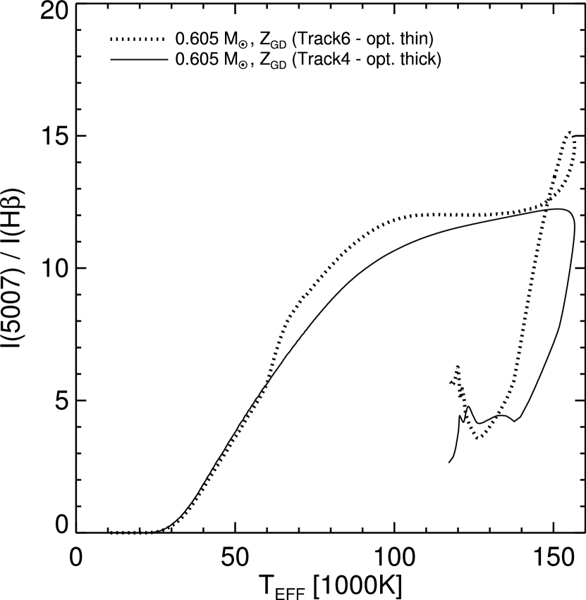
Figure 2: I(5007)/I(H$\beta$) line ratio vs central star effective temperature for two hydrodynamical sequences calculated in SJSS07. $Z_{\rm GD}$ means the metallicity of our Galactic disk. The nebula following Track 4 (solid line) remains always optically thick, while along Track 6 (dotted line) the nebula becomes optically thin to H-ionizing photons as the central star evolves. The ratio is always larger in the optically thin phase, but the difference is seldom larger than about 10% in the relevant bright phases.

Having generated random numbers that give post-AGB ages and central star masses, we derive for each central star the corresponding luminosity and effective temperature, using H-burning post-AGB evolutionary tracks by Schönberner (1989) and Blöcker (1995) to build a look-up table and an associated bilinear interpolation procedure. For example, Figure 2 in Méndez & Soffner (1997) shows the resulting values of luminosity and temperature for the central stars of randomly generated PNs.

2.3 Nebular H$\beta$ luminosities and UV photon leaking

Knowing $L$ and $T_{\rm eff}$, we calculate, using recombination theory, the H$\beta$ luminosity that the nebula would emit if it were completely optically thick in the H Lyman continuum. Then we generate a random number, subject to several conditions (derived from observations of Galactic PNs and their central stars; see next subsection and Méndez et al. 1992), for the absorbing factor $\mu$, which gives the fraction of stellar ionizing luminosity absorbed by the nebula. We use the absorbing factor to correct the nebular H$\beta$ luminosity for the effect of UV photon leaking. We consider the factor $\mu$ to be essential for a successful PNLF simulation, for two reasons. First, after the Hubble Space Telescope images, we know that most PNs show equatorial density enhancements, suggesting that even if they are optically thick in the direction of the equator, they are likely to start leaking UV ionizing radiation through the poles very soon. Second, we can show (Méndez & Soffner 1997) that a PNLF generated under the assumption that all PNs are completely optically thick in all directions turns out to be too bright. Can we reduce the maximum final mass, instead of allowing for UV photon leaking? No, because such massive central stars are known to exist; their suppression is not an option. Can we attribute the weakening to circumstellar dust extinction? The answer to this question is more complicated. Circumstellar dust extinction is probably a dominant factor for the most massive central stars in regions with recent star formation; as we mentioned at the end of subsection 2.1, this probably helps to understand why the bright end of the PNLF is not substantially brighter than in galaxies without recent star formation. However, we should expect circumstellar dust extinction to become less important as we consider less massive central stars. These less massive central stars are expected to evolve more slowly, giving time for the ejected material to dissipate.

At this point we need to introduce the observed behavior of the recombination line H$\beta$. Consider the PNs with the brightest H$\beta$ fluxes in the Magellanic Clouds, as shown in Figure 4a of Dopita et al. (1992). Some of them are of low excitation class, which indicates central star surface temperatures around 30,000 K. We know that, for constant luminosity, the number of H-ionizing photons from the central star increases roughly by a factor 2.5 as we go from $T_{\rm eff}$ = 30,000 K to 70,000 K. The nebular H$\beta$ luminosity is nearly proportional to the number of H-ionizing photons. For that reason we expect a completely optically thick nebula to show an increasing H$\beta$ luminosity as its central star heats up. If we want to keep the low-excitation PNs among the brightest in H$\beta$, we need increasing UV photon leaking at higher $T_{\rm eff}$. Note that here circumstellar dust extinction does not help, because we expect more extinction at lower $T_{\rm eff}$ and less extinction as the central star heats up and the nebula expands. We conclude that, in the case of the Magellanic Clouds PNs, it is the absorbing factor, not circumstellar dust extinction, that plays a predominant role. We assume that this conclusion applies in general. Of course the only way to test this assumption is to obtain deep spectrophotometry of many PNs in different galaxies, which we hope can be done in the not too distant future. Note that for this purpose the search technique must be oriented to detecting PNs in a recombination line like H$\alpha$ or H$\beta$, not just those with strong [O III] emission, which of course will never belong to low excitation classes. For a more detailed discussion on the interpretation of H$\beta$ luminosities, please refer to section 6 “Consistency checks” in Méndez & Soffner (1997).

2.4 More about the absorbing factor

For easier reference, we repeat here some information given in previous papers. The empirical basis for the assignment of absorbing factors is a study of optical thickness in Galactic PNs (Méndez et al. 1992). We generate absorbing factors $\mu$ using random numbers. For $T_{\rm eff}$s between 25,000 and 40,000 K, $\mu$ follows a random uniform distribution between 0.4 and 1.4, with all values higher than 1 replaced by 1. This produces a certain predominance of completely optically thick objects, as observed in Table 4 of Méndez et al. (1992), but allows for the observed fraction of optically thin PNs with low-$T_{\rm eff}$ central stars. For $T_{\rm eff}$s between 40,000 K and the beginning of the white dwarf cooling track, $\mu$ follows a random uniform distribution between 0.05 and the parameter $\mu_{\rm max}$. We adopt $\mu_{\rm max}=1$; in this way some percentage of the bright PNs with very hot central stars can have $\mu$ close to 1. For central stars on the white dwarf cooling tracks, $\mu$ is set equal to a random number uniformly distributed between 0.1 and 1, and this number is multiplied by a factor (1$-$(age(years)/30,000)). In this way we ensure that $\mu$ tends to 0 as the nebula dissipates.

We have kept the random generation of $\mu$ as simple as possible, because the amount of empirical information is quite limited. There is no explicit influence of the central star mass, for example, basically because we lack credible empirical information that could guide our modeling. It will always be possible to complicate the computer codes once more information becomes available. For the moment our simple procedure appears to work well. Although our physical interpretation of the absorbing factor is open to future refinements, we would like to emphasize that once we introduce the absorbing factor, as constrained by the information we have about optical thickness of PNs in our Galaxy, the PNLF we generate agrees with the observed ones, without any further adjustment.

2.5 The intensity ratios [O III]$\lambda$5007/H$\beta$

Since we have generated the H$\beta$ luminosities, now we only need to generate the ratios $\lambda$5007/H$\beta$ to obtain the $\lambda$5007 luminosities and compute the PNLF. At this point we depart from Méndez & Soffner (1997). They used mostly random numbers to generate the intensity ratios, in such a way that the observed histograms of $\lambda$5007/H$\beta$ ratios in our Galaxy and the LMC could be approximately reproduced. Instead, we want to calculate our $\lambda$5007/H$\beta$ ratios from hydrodynamical PN models (Schönberner et al. 2007). Several evolutionary sequences of model PNs have been constructed, one sequence for each of a limited number of central star masses. In the following sections we briefly review the basic characteristics of these models, and we explain the interpolation procedure we have implemented to obtain $\lambda$5007/H$\beta$ ratios for any combination of post-AGB age and central star mass. In this way we move one step closer to a physically consistent procedure for the generation of a PNLF.

3 Modeling the PN evolution

The PN model sequences produced by Schönberner et al. (2007, in what follows SJSS07) are based on coupling a spherical circumstellar envelope, assumed to be the relic of a strong AGB wind, to a H-burning post-AGB model, and following the evolution of the whole system across the H-R diagram toward the white-dwarf cooling track. The goal is to produce radiation-hydrodynamics simulations with the proper initial and boundary conditions. A one-dimensional radiation-hydrodynamics code is employed (Perinotto et al. 1998). This code is designed to compute ionization, recombination, heating, and cooling, fully time-dependently. The chemical composition is typical for Galactic disk PNs (slightly below solar; see Table 1 in SJSS07). Nebular evolutionary sequences have been computed for central stars with masses 0.565, 0.585 (unpublished), 0.595, 0.605, 0.625 and 0.696 $M_{\odot}$. Their corresponding post-AGB evolutionary tracks in the HR diagram are shown in Figure 1.

Although the models are spherically symmetric, they represent the observed nebular structures, as indicated by the H$\alpha$ brightness distributions, extremely well. These nebular models show in many cases a transition between optically thick and thin in the Lyman continuum. Note, however, that it is not clear if the models can accurately predict what fraction of the H-ionizing radiation is being lost through the nebular poles, due to departures from spherical symmetry in the real nebulae. At this point it looks better to use the absorbing factors $\mu$ as defined by Méndez et al. (1992, 1993), and combine them with intensity ratios $\lambda$5007/H$\beta$, which are not too much affected by the onset of UV photon leaking; see Figure 2. We believe that a combination of spherically symmetric nebula plus $\mu$ absorbing factor may be a good compromise to describe the evolution of PNs in a more realistic way than previously attempted, without having to introduce the enormous complexities of two-dimensional hydrodynamics.

In summary, here we use the SJSS07 model sequences for one purpose only: to obtain the intensity ratio $\lambda$5007/H$\beta$ as a function of nebular post-AGB age. The resulting run of this ratio for the six central star masses is shown in Figure 3. Next step is to implement an interpolation procedure that will provide similar information for any central star mass.

4 Interpolation method for the generation of $\lambda$5007/H$\beta$

To begin with, we have a table giving central star surface temperature $T$, central star luminosity $L$, and nebular ratio $\lambda$5007/H$\beta$, which we will call $R$, as a function of post-AGB age $t$, for each of the six central star masses listed above. The interpolation between these tracks is done following a technique described by van der Sluys et al. (2005). We first divide each of the nebular evolutionary tracks shown in Figure 3 into three sections: (a) where $R$ increases until it reaches a maximum; (b) where $R$ decreases; (c) where $R$ stabilizes. There is one exception: since the transition between 0.595 and 0.585 $M_{\odot}$ is somewhat different, in that case we have modified (b) and (c) in the following way: (b) where $R$ is between the two peaks; (c) where $R$ decreases.

For each of these 3 sections we define a path length $l$ by the following expression:

$$l=\sum_{i}\sqrt{\Big{(}\frac{t(i)-t(i-1)}{\Delta t}\Big{)}^{2}+\Big{(}\frac{R(i)-R(i-1)}{\Delta R}\Big{)}^{2}}$$ (1)

In this equation, $i$ is the index corresponding to the successive data rows in each table, and the quantities $\Delta t$ and $\Delta R$ are the total increments in $t$ and $R$ between the beginning and end of each section.

Each of these 3 sections is redistributed into a fixed number of data points, equally spaced in the path length. The values for these equally spaced points are calculated by polynomial interpolation along each track. Having done this, each section of each nebular evolutionary track has the same number of data points, and one point in any section, like (a) to fix ideas, marks an evolutionary state similar to that of the same point along the (a) section in any other nebular evolutionary track.

Now we are able to interpolate between adjacent nebular evolutionary tracks, building point by point a new track for each randomly generated central star mass. Figure 3 shows two simulated tracks, in the $R$-$t$ plane, produced with this interpolation technique. Their corresponding central star post-AGB evolution in the HR diagram is also plotted in Figure 1. Once in posession of the time evolution of $R$ for any randomly generated central star mass, we can obtain $R$ for the randomly generated post-AGB age, and we can proceed to build the PNLF.

5 Results and discussion

Our ultimate purpose is to generate a physically consistent PNLF, eliminating as much as possible the random numbers used in previous modeling, which were reflecting our lack of information about the evolution and properties of the PNs at each specific moment. At the present time we cannot produce a fully satisfactory simulation, because we would need first to explore variations in many input parameters and their effect on the PN evolution. For example, we cannot discuss metallicity effects until we have nebular evolutionary tracks for a broad range of metallicities. But we would like to show the very promising results of a simulation based on the limited number of nebular evolutionary tracks presented by SJSS07.

First of all we consider the histogram of the intensity of [O III]$\lambda$5007, on the scale $I({\rm H}\beta)=100$. On this scale, $I$(5007) is equivalent to 100 $R$. In previous work, we simulated the observed histograms of $I$(5007) in our Galaxy and the LMC using predominantly random numbers. Can we obtain a satisfactory fit to the observations using instead the ratios $R$ generated by our PN evolution programs? Before attempting that, we need to consider selection effects: which of our generated PNs would actually be observable? We seek guidance in Figure 4, which is a modified version of Figure 13 in SJSS07 (we could have used their Figure 14 instead), showing the excitation class (defined in Eq. (2) of SJSS07) as a function of the nebular absolute magnitude $M$(5007). Note that the observed PNs are enclosed by the nebular evolutionary tracks corresponding to central star masses of 0.696 and 0.585 $M_{\odot}$. Nebulae that belong to less massive central stars fail to become bright, because the central stars evolve very slowly away from the AGB, and the nebulae dissipate, becoming very optically thin, and displaying a very low surface brightness. This indicates that they are probably missing in the observed samples.

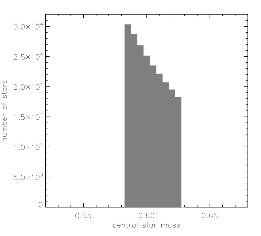
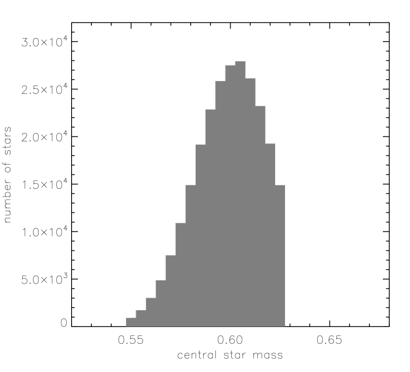
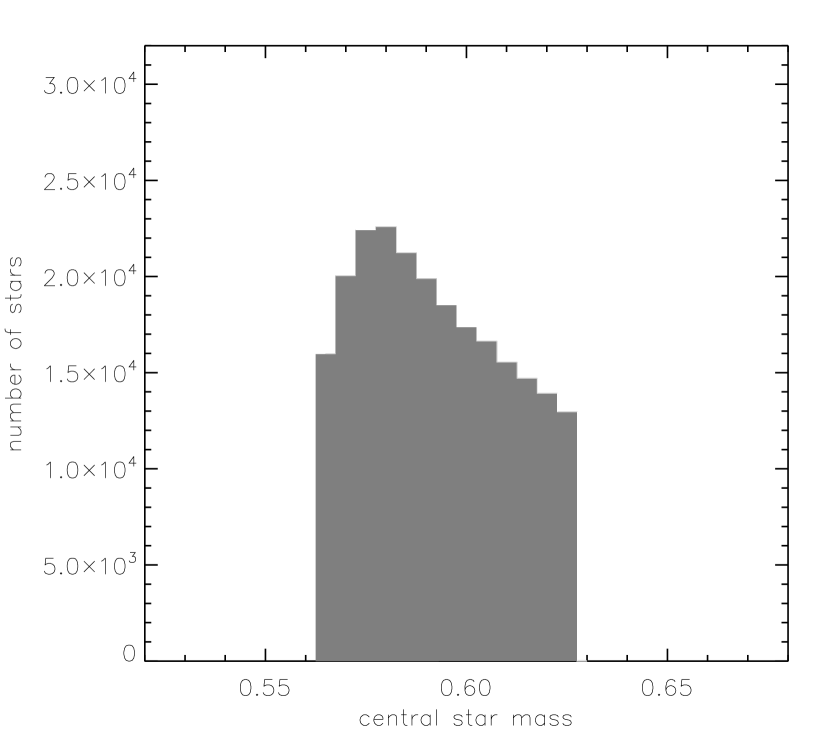
Figure 8: PNLFs generated using different central star mass distributions. The mass distributions are on the left, and the corresponding PNLFs (full lines) are on the right. The first (upper) mass distribution is the one used to produce Fig. 7, with a sharp low-mass cut at 0.585 $M_{\odot}$. The 2nd and 3rd include progressively more low-mass central stars. The three PNLFs are compared with the old PNLF generated as in Méndez and Soffner (1997), indicated with a dash-dotted line. As we increase the number of low-mass stars, the PNLF becomes more similar to the old one.

Thus, in building the theoretical distribution of $I$(5007), in order to be consistent with the nebular properties that result from the initial and boundary conditions assumed in SJSS07, we have decided to eliminate the contribution from all central stars less massive than 0.585 $M_{\odot}$. The central star mass distribution we adopted will be shown later (see the upper mass distribution in Figure 8). We have also eliminated all PNs with central stars fainter than log $L/L_{\odot}$ = 2.4. This was done, in the same way as in Méndez & Soffner (1997), in order to compensate for an obvious selection effect: the observed distributions in our Galaxy and in the LMC are not likely to include PNs with very low-L central stars, all of which have high surface temperatures.

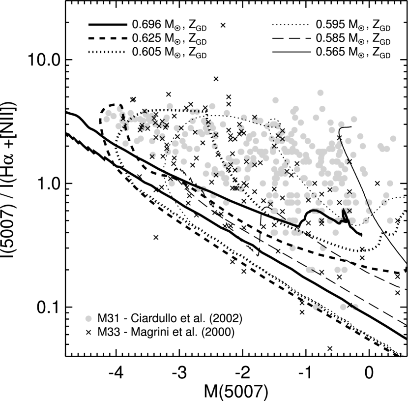
Figure 6: [O III] $\lambda$5007 to H$\alpha$ + [N II] line ratios for PNs in the M 31 bulge and M 33. The data, taken from Ciardullo et al. (2002) and Magrini et al. (2000), are compared with PN evolutionary tracks from SJSS07. $Z_{\rm GD}$ means the metallicity of our Galactic disk. Evolution is from lower right to upper left and back. The models cover the observed range very well; no internal reddening corrections are needed. The reason for the small number of PNs near the upward-moving tracks is that the probability of finding them there is low. Please refer to SJSS07 (section 5 and figure 15). The PN brightens quickly, and then it fades more slowly, so that we find most of the observed PNs in the fading region.

Figure 5 shows, then, our corrected theoretical distribution, compared with two observed distributions: one for 118 PNs in the LMC (data taken from Wood et al. 1987; Meatheringham et al. 1998; Jacoby et al. 1990; Meatheringham & Dopita 1991a, 1991b; Vassiliadis et al. 1992) and another one for 983 PNs in our Galaxy, taken from the Strasbourg-ESO Catalogue of Galactic PNs (Acker et al. 1992). These are the same two distributions used in Figure 3 of Méndez & Soffner (1997). Our new distribution provides a quite satisfactory fit. We do not expect a perfect fit, of course, because there are even differences between the two observed distributions, the reasons for which are not clear at the present time. Prompted by the anonymous referee, we also show in Figure 6 that the nebular model sequences in SJSS07 can predict the observed distribution of PNs in a diagram of the [O III] $\lambda$5007 to H$\alpha$ + [N II] line ratio as a function of $M$(5007), like the one shown in Fig. 2 of Ciardullo et al. (2002).

Since we have been able to produce a value of $I$(5007) for every pair of values of post-AGB age and central star mass in our simulations, we can proceed to build the new $\lambda$5007 PNLF. Figure 7 shows a comparison between the old PNLF (Méndez & Soffner 1997) and the new one. The agreement between the two simulations at the bright end is excellent. There is a difference at fainter magnitudes, which does not affect the use of the PNLF for distance determinations.

What is the nature of the “camel shape” apparent in the new simulation? It can be described as a relative lack of PNs for $M$(5007) between $-3$ and 0. In fact, it was already present in the Méndez & Soffner (1997) simulations, but it is more pronounced here. We believe that the most natural explanation of this deficit of PNs at intermediate luminosities is related to the fact that the central stars in our simulation are shell H-burners. See Section 9 in Méndez (1999). Post-AGB evolutionary tracks show a quick drop in luminosity as the H-burning shell is extinguished and the star goes into the white dwarf cooling track. For that reason there is a lack of central stars at log $L/L_{\odot}$ below 3.5. This lack of central stars at intermediate luminosities can explain the lack of intermediate-brightness PNs in the PNLF.

If this explanation is correct, then it should also explain the different shapes in Figure 7. The most important difference between the new and the old simulation is that the old one uses a central star mass distribution extending down to masses as low as 0.55 $M_{\odot}$. The luminosity drop suffered by H-burning central stars is in fact much less dramatic for lower-mass central stars, and therefore we expect such low-mass central stars to help reduce the deficit, as observed in Figure 7.

Let us show this effect in more detail. In Figure 8 we show three simulations. The first one uses a central star mass distribution with a sharp low-mass cut at 0.585 $M_{\odot}$. In the 2nd and 3rd cases we allow the mass distribution to be extended toward less massive central stars. Since SJSS07 cannot be used at these low masses, because the nebulae are predicted to be too faint, for these low-mass central stars we used the procedure of Méndez and Soffner (1997) to generate the values of the ratios $\lambda$5007/H$\beta$. Indeed it appears that the addition of more and more lower-mass central stars increasingly reduces the deficit, as expected. Of course we would need to investigate if it is possible to impose reasonable initial conditions that will result in visible PNs around the lower-mass central stars. We assume that this is possible, but such an investigation is extremely time-consuming and lies outside the scope of the present work.

We should mention in passing that another way of decreasing the deficit is to allow for a certain percentage of He-burning central stars, which do not show a quick luminosity drop. We cannot include such evolutionary tracks in our procedure; see Méndez & Soffner (1997) and the discussion (section 7) in SJSS07.

The new PNLF shape we have obtained reminds us immediately of the observed PNLF in the SMC as described by Jacoby & De Marco (2002). Therefore in Figure 9 we fit the Jacoby & De Marco data with our new PNLF. The agreement is very encouraging. The fit to the bright end gives a distance modulus of 19.3 mag, which agrees, within the rather large uncertainties, with the 19.1 obtained by Jacoby et al. (1990, see in particular their Figure 5). Whenever we fit the PNLF we are making a simultaneous fit to both the distance modulus and to the total number of PNs in the galaxy in question; thus our new simulation also implies a total number of approximately 120 PNs in the surveyed area of the SMC, in rough agreement with estimates by Jacoby and De Marco (2002). Note that the PN numbers observed at faint magnitudes are probably affected by some incompleteness; we are fitting only the bright end of the SMC PNLF, which appears to be complete, as discussed by Jacoby and De Marco.

In Figure 9 we find that the mass distribution with a sharp cut at 0.585 $M_{\odot}$ gives a better fit than other distributions that include a contribution from lower central star masses. A lack of low-mass central stars in the SMC may have different possible interpretations. It might reflect lack of star formation at earlier times, producing a lack of the corresponding low initial masses (Ciardullo et al. 2004); it might also mean that, in the SMC, low-mass central stars find it more difficult to produce visible PNs, perhaps as a consequence of the low metallicity. These ideas will have to be tested when nebular evolution models like those of SJSS07, but for lower metallicities, become available. The PNLF shape may provide useful diagnostics for studies of star formation history and post-AGB evolution in different populations.

6 Recapitulation and perspectives

We have shown that using models like those of SJSS07 it is possible to generate a numerical simulation of a PNLF, if we are willing to assume an empirically given central star mass distribution, which however still needs to be justified from stellar evolution and population evolution theories. Leaving that problem aside, the new procedure is able to reproduce observed histograms of $I$(5007), and the new generated PNLF agrees with the old one at the bright end, which means that it gives the same PNLF distances as before. In addition, we have found that the shape of this new simulated PNLF explains the observed PNLF shape in the SMC quite well.

What remains to be done is to systematically explore the initial parameters controlling the PN model evolution, to see what effects they have on the PNLF. In particular, initial conditions may influence the low-mass cut we need to apply in the central star mass distribution, probably in part as a function of metallicity.

The results we have presented offer some promise for future PNLF research. Most important, if it is possible to produce new PN evolution models for a variety of metallicities (a difficult task, because it requires at the very least to have a good theoretical treatment of AGB and post-AGB mass loss, in order to deal with both central star and nebular evolution), then it will become comparatively easy, using the methods described here, to investigate metallicity effects on the PNLF. If it is possible to build observed PNLFs for several galaxies down to fainter magnitudes, then the different PNLF shapes, if confirmed, would provide a very useful diagnostic for population characteristics like star formation history, central star mass distribution of observable PNs, or perhaps even the relative frequency of He-burners among PN central stars.

Figure 1: Solid lines are post-AGB evolutionary tracks for six central star masses in the log $T_{eff}$–log $L$ plane. Dashed lines (unlabeled) are two interpolated tracks generated as in Méndez & Soffner (1997).

Figure 3: Solid lines are PN evolutionary tracks for the six central star masses, taken from SJSS07, in the $t$–$I$(5007) plane; $I$(5007) is on the scale $I(H\beta)$=100. The dashed lines (unlabeled) are two interpolated tracks, each corresponding to one of the interpolated stellar evolutionary tracks shown in Fig. 1. The interpolated PN evolutionary track generation is explained in Section 4.

Figure 4: Nebular excitation parameter vs. absolute $\lambda$5007 magnitude, for five hydrodynamical sequences labeled according to their mass. Open circles along the tracks indicate the moment when the nebular models become optically thin for Lyman continuum photons. The gaps seen for some tracks are artifacts caused by the definition of the excitation parameter (see also SJSS07, Figs. 13 and 14 therein). Data of Galactic PNs with spectroscopically determined distances are shown as dots for comparison. This figure is a modified version of Fig. 13 in SJSS07. The ’circled’ dot belongs to NGC 7293, the two ’squared’ dots to the high-excitation PNs NGC 1360 and NGC 4361. The filled triangle marks the position of NGC 7027.

Figure 5: Histograms of the intensity of $\lambda$5007, on the scale $I(H\beta)$=100. The dashed line indicates the histogram for 983 objects in our Galaxy. The other two histograms have been normalized to this number. The dotted line is the histogram for 118 LMC objects. The full line is our new distribution, generated as described in the text.

Figure 7: PNLF (full line) generated using the hydrodynamical models by SJSS07, compared with the old PNLF (dashed line) generated as described in Méndez & Soffner (1997).

Figure 9: Fits to the 59 PNs found in the SMC by Jacoby and De Marco (2002) with the new PNLF simulations. The PNLF binning is broad (1 mag) due to the small number of PNs. The fainter bins are probably affected by incompleteness in the SMC surveys. The left figure, which provides a better fit, corresponds to the upper central star mass distribution in Fig. 8, with the sharp low-mass cut at 0.585 $M_{\odot}$. The fit was obtained adopting a distance modulus $m-M$ = 19.34. The three lines are PNLF simulations for three different sample sizes: 70, 120, 190. The right figure corresponds to the 3rd central star mass distribution in Fig. 8. The fit was obtained adopting a distance modulus $m-M$ = 19.25, and the sample sizes are 30, 75 and 150. In both figures we fit only the bright end of the PNLF, as discussed in the text.

References

- (1) Acker, A., Ochsenbein, F., Stenholm, B., et al. 1992, The Strasbourg-ESO Catalogue of Galactic PNs
- (2) Alves, D.R., Bond, H.E., & Livio, M. 2000, AJ, 120, 2044
- (3) Blöcker, T. 1995, A&A, 299, 755
- (4) Ciardullo, R. 2003, in IAU Symposium 209, Planetary Nebulae: their evolution and role in the universe, ed. S. Kwok, M. Dopita & R. Sutherland (San Francisco: ASP), 617
- (5) Ciardullo, R. 2006, in IAU Symposium 234, Planetary Nebulae in our Galaxy and beyond, ed. M.J. Barlow & R.H. Méndez (Cambridge University Press), 325
- (6) Ciardullo, R., Durrell, P.R., Laychak, M.B., et al. 2004, ApJ, 614, 167
- (7) Ciardullo, R., Feldmeier, J.J, Jacoby, G.H., et al. 2002, ApJ, 577, 31
- (8) Ciardullo, R., Jacoby, G.H., Ford, H.C., & Neill, J.D. 1989, ApJ, 339, 53
- (9) Ciardullo, R., Sigurdsson, S., Feldmeier, J.J, & Jacoby, G.H. 2005, ApJ, 629, 499
- (10) Dopita, M.A., Jacoby, G.H., & Vassiliadis, E. 1992, ApJ, 389, 27
- (11) Ferrario, L., Wickramasinghe, D., Liebert, J., & Williams, K.A. 2005, MNRAS, 361, 1131
- (12) Jacoby, G.H. 1989, ApJ, 339, 39
- (13) Jacoby, G.H. & Ciardullo, R. 1999, ApJ, 515, 169
- (14) Jacoby, G.H. & De Marco, O. 2002, AJ, 123, 269
- (15) Jacoby, G.H., Walker, A.R., & Ciardullo, R. 1990, ApJ, 365, 471
- (16) Magrini, L., Corradi, R.L.M., Mampaso, A., & Perinotto, M. 2000, A&A, 355, 713
- (17) Marigo, P., Girardi, L., Weiss, A., et al. 2004, A&A, 423, 995
- (18) McCarthy, J.K., Méndez, R.H., Becker, S., et al. 1997, in IAU Symposium 180, Planetary Nebulae, ed. H.J. Habing & H.J.G.L.M. Lamers (Dordrecht: Kluwer), 122
- (19) Meatheringham, S.J., & Dopita, M.A. 1991a, ApJS, 75, 407
- (20) Meatheringham, S.J., & Dopita, M.A. 1991b, ApJS, 76, 1085
- (21) Meatheringham, S.J., Dopita, M.A., & Morgan, D.H. 1988, ApJ, 329, 166
- (22) Méndez, R.H. 1999, in Post-Hipparcos Cosmic Candles,, ed. A. Heck & F. Caputo (Dordrecht:Kluwer), 161
- (23) Méndez, R.H., Kudritzki, R.P., Ciardullo, R., & Jacoby, G.H. 1993, A&A, 275, 534
- (24) Méndez, R.H., Kudritzki, R.P., & Herrero, A. 1992, A&A, 260, 329
- (25) Méndez, R.H., & Soffner, T. 1997, A&A, 321, 898
- (26) Méndez, R.H., Thomas, D., Saglia, R.P., et al. 2005, ApJ, 627, 767
- (27) Meng, X., Chen, X., & Han, Z. 2007, astro-ph 0710.2397
- (28) Perinotto, M., Kifonidis, K., Schönberner, D., & Marten, H. 1998, A&A, 332, 1044
- (29) Schönberner, D. 1989, in IAU Symposium 131, Planetary Nebulae, ed. S. Torres-Peimbert (Dordrecht: Kluwer), 463
- (30) Schönberner, D., Jacob, R., Steffen, M., & Sandin, C. 2007, A&A, 473, 467
- (31) van der Sluys, M.V., Verbunt, F., & Pols, O.R. 2005, A&A, 431, 647
- (32) Vassiliadis, E., Dopita, M.A., Morgan, D.H., & Bell, J.F. 1992, ApJS, 83, 87
- (33) Weidemann, V. 2000, A&A, 363, 647
- (34) Wood, P.R., Meatheringham, S.J., Dopita, M.A., & Morgan, D.H. 1987, ApJ, 320, 178