Evolution of low-frequency features in the CMB spectrum due to stimulated Compton scattering and Doppler-broadening

We discuss a new solution of the Kompaneets-equation for physical situations in which low frequency photons, forming relatively narrow spectral details, are Compton scattered in an isotropic, infinite medium with an intense ambient blackbody field that is very close to full thermodynamic equilibrium with the free electrons. In this situation the background-induced stimulated Compton scattering slows down the motion of photons toward higher frequencies by a factor of $3$ in comparison with the solution that only takes into account Doppler-broadening and boosting. This new solution is important for detailed computations of cosmic microwave background spectral distortions arising due to uncompensated atomic transitions of hydrogen and helium in the early Universe. In addition we derive another analytic solution that only includes the background-induced stimulated Compton scattering and is valid for power-law ambient radiation fields. This solution might have interesting applications for radio lines arising inside of bright extra-galactic radio source, where according to our estimates line shifts because of background-induced stimulated scattering could be amplified and even exceed the line broadening due to the Doppler-effect.

1 Introduction

The recombination of He III ($4500\lesssim z\lesssim 7000$) in the Universe produces specific quasi-periodic distortions of cosmic microwave background (CMB) in the Rayleigh-Jeans part of the CMB spectrum, at dm and cm wavelength (Dubrovich & Stolyarov, 1997; Rubino-Martin et al., 2007). It is also well-known that any energy release below $z\sim 5\times 10^{4}$ will lead to a characteristic broad $y$-type distortion (Zeldovich & Sunyaev, 1969) of the background radiation. In this case because of uncompensated loops (Lyubarsky & Sunyaev, 1983), trying to restore full equilibrium, similar features should originate from even higher redshifts (Chluba & Sunyaev, 2008). However, their amplitude and phase-dependence should differ from those of the distortions arising during He III recombination.

It is clear that in both cases the multiple scattering of photons by hot electrons should lead to broadening and shifting of these spectral features. Here we investigate the evolution of narrow lines due to both stimulated scattering in the presence of the much brighter CMB background with temperature $T_{\gamma}=2.7\,(1+z)\,$K, and Doppler-broadening and boosting. According to our analytical solutions, in this situation the background-induced stimulated Compton scattering at low frequencies slows down the motion of photons toward higher frequencies by a factor of $3$ in comparison with the solution that only takes into account Doppler-broadening and boosting (Zeldovich & Sunyaev, 1969).

We present two analytical solutions demonstrating this fact. In the first we only include the pure effect of stimulated scattering in the presence of a bright power-law ambient photon field, neglecting the Doppler-effect (see Sect. 3), while in the second solution we take into account both effects simultaneously, but restrict ourselves to the case of a low-frequency blackbody ambient photon field with temperature $T_{\gamma}\sim T_{\rm e}$, where $T_{\rm e}$ denotes the electron temperature (see Sect. 4). The second solution also clearly shows that the broadening of the weak lines in this situation depends only on the $y$-parameter defined by $T_{\rm e}$, even though the evolution of the ambient CMB blackbody spectrum itself is described by $y\propto T_{\rm e}-T_{\gamma}$.

2 Summary of previous analytic solutions to the Kompaneets-Equation

The repeated Compton scattering of photons by thermal electrons in isotropic, infinite media can be described using the well-known Kompaneets-equation (Kompaneets, 1956)

$$\frac{\displaystyle\partial n(x_{\rm e},{y_{\rm e}})}{\displaystyle\partial{y_{\rm e}}}=\frac{1}{x_{\rm e}^{2}}\,\frac{\displaystyle\partial}{\displaystyle\partial x_{\rm e}}\,x_{\rm e}^{4}\left[\frac{\displaystyle\partial n}{\displaystyle\partial x_{\rm e}}+n(1+n)\right]\,,$$ (1)

where $n(x_{\rm e},{y_{\rm e}})=c^{2}I_{\nu}/2h\nu^{3}$ is the photon occupation number, ${y_{\rm e}}=\int\frac{kT_{\rm e}}{m_{\rm e}c^{2}}\,N_{\rm e}\sigma_{\rm T}c{\,\rm d}t$ is the Compton $y$-parameter, where $T_{\rm e}$ denotes the electron temperature, and $x_{\rm e}=h\nu/kT_{\rm e}$ is the dimensionless frequency.

As is well understood, the first term in brackets ($\propto\partial_{x_{\rm e}}n$) describes the diffusion of photons along the frequency axis, the second term ($\propto n$) the motion of photons towards low frequencies due to the recoil-effect, and the last term ($\propto n^{2}$) the effect of stimulated scattering, which physically is also related to recoil (e.g. see Sazonov & Sunyaev, 2000). Eq. (1) has been studied in great detail, both numerically (e.g. Pozdniakov et al., 1983) and analytically in several limiting cases, but, to our knowledge, no general analytic solution was found.

In situations when the recoil-term and stimulated scatterings are not important (i.e. $n[n+1]\ll\partial_{x_{\rm e}}n$), Zeldovich & Sunyaev (1969) gave a solution for arbitrary value of ${y_{\rm e}}$, which reads

$$\left.n(\nu,{y_{\rm e}})\right|_{\rm diff}=\frac{1}{\sqrt{4\pi\,{y_{\rm e}}}}\int n_{0}(\tilde{\nu})\,e^{-\textstyle\frac{(\ln[\nu/\tilde{\nu}]+3{y_{\rm e}})^{2}}{4\,{y_{\rm e}}}}\,\frac{{\rm d}\tilde{\nu}}{\tilde{\nu}}\,.$$ (2)

Here $n_{0}(\nu)$ is the photon occupation number at frequency $\nu$ and ${y_{\rm e}}=0$. For ${y_{\rm e}}\ll 1$ the broadening of an initially narrow line is given by $\Delta\nu/\nu\sim\pm 2\sqrt{{y_{\rm e}}\,\ln 2}$. Due to Doppler-boosting, the maximum of the specific intensity $I_{\nu}$ moves along $\nu_{\rm line}({y_{\rm e}})=\nu_{0}\,e^{3{y_{\rm e}}}$, so that for ${y_{\rm e}}\ll 1$ one has $\Delta\nu/\nu\sim 3{y_{\rm e}}$, implying that photons are upscattered.

In the case when the diffusion term and stimulated scatterings are not important, Arons (1971) and independently Illarionov & Syunyaev (1972), using different mathematical approach, gave a solution which can be written in the form

$$\left.n(\nu,\tau_{\rm T})\right|_{\rm recoil}=\frac{1}{[1-\omega\,\tau_{\rm T}]^{4}}\,n_{0}\left(\frac{\nu}{1-\omega\,\tau_{\rm T}}\right)\,,$$ (3)

where $\omega=\frac{h\nu}{m_{\rm e}c^{2}}$ and $\tau_{\rm T}=N_{\rm e}\sigma_{\rm T}c\,t$ is the Thomson-scattering optical depth. This solution simply describes the motion of photons towards lower frequencies, where for initial photon distribution, $n_{0}(\nu)=A\,\delta(\nu-\nu_{0})/\nu^{2}$, at later time the line is located at $\nu_{\rm line}(\tau_{\rm T})=\nu_{0}/[1+\omega_{0}\tau_{\rm T}]$. For $\omega\tau_{\rm T}\ll 1$ the line shift due to recoil is given by $\Delta\nu/\nu\sim-\omega\tau_{\rm T}$. This shows that at low frequencies ($h\nu\ll kT_{\rm e}$) the recoil-effect can be neglected in comparison with Doppler-boosting.

The third analytic solution was found in the case when only the stimulated scattering term is important (Zeldovich & Levich, 1968; Sunyaev, 1970). Here the solution is determined by the implicit equation

$$\nu=\phi(f)-2\,\frac{h}{m_{\rm e}c^{2}}\,\tau_{\rm T}\,f\,,$$ (4)

with $f(\nu,\tau_{\rm T})=\nu^{2}\,n(\nu,\tau_{\rm T})$ and where $\phi(z)$ can be found from the initial condition ($\phi(z)\equiv f^{-1}_{0}(z)$, where $f^{-1}_{0}(z)$ is the inverse function of $f(\nu,\tau_{\rm T})$ at $\tau_{\rm T}=0$).

Note that the last two solutions do not depend on the temperature of the electrons, since in both cases physically the motion of the electrons in lowest order does not play any role.

3 Solution for purely background-induced stimulated scattering

In this Section we discuss the situation when photons from a low-frequency spectral feature are scattering off thermal electrons at temperature $T_{\rm e}$ within an intense photon background that has a power-law spectral dependence, i.e. ${n_{\rm back}}(\nu)={A_{\rm back}}\,\nu^{\beta}\gg 1$. Here $n_{0,\rm back}={A_{\rm back}}\nu_{0}^{\beta}\gg 1$ is the occupation number of background photon field in the vicinity of the spectral feature at $\nu_{0}$, and $\beta$ denotes the power-law index.

If we neglect the evolution of the background photon field and assume that recoil and Doppler broadening are negligible, then, inserting $n={n_{\rm back}}+\Delta n$ into Eq. (1), one is left with

$$\frac{\displaystyle\partial\Delta n(\nu,\tau_{\rm T})}{\displaystyle\partial\tau_{\rm T}}\!\approx\!\frac{2}{\nu^{2}}\,\frac{h}{m_{\rm e}c^{2}}\,\frac{\displaystyle\partial}{\displaystyle\partial\nu}\,\nu^{4}\,{n_{\rm back}}(\nu)\,\Delta n\,.$$ (5)

For initial photon distribution $\Delta n_{0}(\nu)=\Delta n(\nu,\tau_{\rm T}=0)$ the solution is given by

$$\left.\Delta n(\nu,\tau_{\rm T})\right|_{\rm back-ind}=\frac{\Delta n_{0}\left(\frac{\nu}{[1-2(\beta+1)\,{n_{\rm back}}(\nu)\,\omega\,\tau_{\rm T}]^{\frac{1}{\beta+1}}}\right)}{[1-2(\beta+1)\,{n_{\rm back}}(\nu)\,\omega\,\tau_{\rm T}]^{\frac{\beta+4}{\beta+1}}}\,.$$ (6)

This solution describes the purely background-induced motion of photons along the frequency axis. Due to the large factor $2\,{n_{\rm back}}\gg 1$ the speed of this motion is increased, so that even for $\omega\tau_{\rm T}\ll 1$ the line shift can still be considerable. For $\beta>-1$ this solution is valid only at $\nu<1/[2(\beta+1)\,{A_{\rm back}}\,\frac{h\tau_{\rm T}}{m_{\rm e}c^{2}}]^{1/(\beta+1)}$.

For initial photon distribution, $\Delta n_{0}(\nu)=A\,\delta(\nu-\nu_{0})/\nu^{2}$, the line is located at $\nu^{\delta}(\tau_{\rm T})=\nu_{0}/[1+2(\beta+1)\,{n_{\rm back}}(\nu_{0})\,\omega_{0}\,\tau_{\rm T}]^{\frac{1}{\beta+1}}$. Here the solution works for all $\beta>-1$, while for $\beta<-1$ it is valid only for $\nu_{0}>[2|\beta+1|\,{A_{\rm back}}\,\frac{h\tau_{\rm T}}{m_{\rm e}c^{2}}]^{1/|\beta+1|}$. For the condition $2(\beta+1)\,{n_{\rm back}}(\nu_{0})\,\omega_{0}\,\tau_{\rm T}\ll 1$ one has $\Delta\nu/\nu_{0}\sim-2\,{n_{\rm back}}(\nu_{0})\,\omega_{0}\,\tau_{\rm T}$. This shows that independent of $\beta$ photons are always moving toward lower frequencies, where the speed of this motion is increased by $2\,{n_{\rm back}}\gg 1$ as compared to the recoil-case (see Sect. 2). It is also remarkable that for $\beta=-1$, i.e. ${n_{\rm back}}\propto 1/\nu$, one has $\Delta\nu/\nu\approx-2\,{A_{\rm back}}\frac{h\tau_{\rm T}}{m_{\rm e}c^{2}}$, so that the line shift is independent of frequency.

It is also possible to rewrite this expression in terms of the brightness temperature

$$T_{\rm b}(\nu)=\frac{c^{2}I_{\nu}^{\rm back}}{2k\nu^{2}}\equiv\frac{h\nu}{k}\,{n_{\rm back}}(\nu),$$ (7)

of the background field in the vicinity of the spectral feature, yielding

$$\left.\frac{\Delta\nu}{\nu}\right|_{\rm back-ind}\sim-2\,\frac{kT_{\rm b}(\nu)}{m_{\rm e}c^{2}}\tau_{\rm T}.$$ (8)

For $T_{\rm b}>\frac{3}{2}T_{\rm e}$, it is clear that the line shift due to background-induced stimulated scattering exceeds the shift towards higher frequencies due to Doppler-boosting. Therefore the net motion of the line center can be directed towards lower frequencies, even if one includes the Doppler-term. Note that for a Rayleigh-Jeans spectrum ${T_{\rm b}}$ is equal to the physical temperature of the radiation field.

Comparing with the case of pure Doppler-broadening (see Sect. 2), it is also clear that for ${y_{\rm e}}\ll 1$ and ${y_{\rm e}}\gtrsim 4\,[T_{\rm e}/T_{\rm b}(\nu)]^{2}\ln 2$ the background-induced line shift becomes larger than the FWHM Doppler-broadening connected with the diffusion term. In this case one can neglect the effect of line-broadening due to the Doppler-term, and, according to Eq. (8), even for small Thomson optical depth can still obtain a rather significant line-shift. In radio spectroscopy is possible to determine tiny shifts or broadening in the frequency of narrow spectral feature (for example of 21 cm lines from high redshift radio galaxies).

3.1 Rayleigh-Jeans limit ($\beta=-1$)

For $\beta=-1$ Eq. (5) becomes $\partial_{\tau_{\rm T}}\Delta n(\nu,\tau_{\rm T})\!=\!\frac{2}{\nu^{2}}\,\frac{h\,{A_{\rm back}}}{m_{\rm e}c^{2}}\,\partial_{\nu}\,\nu^{3}\,\Delta n$, and with the replacement $s=\nu^{3}\,\Delta n$ and $\xi=\ln(\nu)$, can be cast in the form $\partial_{\tau_{\rm T}}s(\xi,\tau_{\rm T})\!=\!\frac{2h\,{A_{\rm back}}}{m_{\rm e}c^{2}}\,\partial_{\xi}s$. Using the characteristic of this equation, or by directly taking the limit $\beta\rightarrow-1$ from Eq. (6), one readily finds

$$\left.\Delta n(\nu,\tau_{\rm T})\right|^{\beta=-1}_{\rm back-ind}=e^{6{A_{\rm back}}\,\frac{h\,\tau_{\rm T}}{m_{\rm e}c^{2}}}\,\Delta n_{0}\left(\nu\,e^{2{A_{\rm back}}\,\frac{h\,\tau_{\rm T}}{m_{\rm e}c^{2}}}\right)\,,$$ (9)

so that for $\Delta n_{0}(\nu_{0})=A\,\delta(\nu-\nu_{0})/\nu^{2}$, the line will be centered at $\nu^{\delta}(\tau_{\rm T})=\nu_{0}\,e^{-2{A_{\rm back}}\,\frac{h\,\tau_{\rm T}}{m_{\rm e}c^{2}}}$. If we assume that ${n_{\rm back}}=kT_{\gamma}/h\nu$, i.e. we are in the Rayleigh-Jeans part of a blackbody photon field with $T_{\gamma}={T_{\rm b}}=T_{\rm e}$, then we have $\nu^{\delta}(\tau_{\rm T})=\nu_{0}\,e^{-2\frac{kT_{\rm e}}{m_{\rm e}c^{2}}\,\tau_{\rm T}}$. This shows that due to stimulated scattering of photons within a blackbody ambient radiation field are moving with a speed $\propto 2{y_{\rm e}}$ towards lower frequencies. This is 3/2 times smaller than the line shift due to Doppler-boosting (see Sect. 2), but is directed in the opposite direction. Below we will discuss this case in more detail, also including the broadening of the line due to the Doppler-effect.

3.2 Evolution of the background-field and the relative velocity of a spectral feature for small line-shifts

In the derivation given above we have neglected the evolution of the background radiation field. This is possible when the line-shifts $\Delta\nu/\nu$ are small. If we insert $n={n_{\rm back}}$ into the Kompaneets-equation (1), and assume that ${y_{\rm e}}$ is sufficiently small, then we can directly write the solution for the change of the photon occupation number as

$$\frac{\Delta{n_{\rm back}}}{{n_{\rm back}}} ={y_{\rm e}}\left\{\beta(3+\beta)+(4+\beta)x_{\rm e}+2{n_{\rm back}}(2+\beta)x_{\rm e}\right\}.$$ (10)

With this one can now find the corresponding overall shift of the background radiation field at initial frequency $x_{\rm e,0}$. Solving the equation ${n_{\rm back}}(x_{\rm e,0})\equiv{n_{\rm back}}(x_{\rm e})[1+\frac{\Delta{n_{\rm back}}(x_{\rm e})}{{n_{\rm back}}(x_{\rm e})}]$, with $x_{\rm e}=x_{\rm e,0}(1+\delta)$, for $\delta\equiv-\Delta\nu/\nu$ under the condition $\beta\neq 0$ one finds:

$$\left.\frac{\Delta\nu}{\nu}\right|_{\rm back} \sim\frac{2\,(2+\beta)}{\beta}\frac{kT_{\rm b}(\nu)}{m_{\rm e}c^{2}}\tau_{\rm T}+\frac{4}{\beta}\,\frac{h\nu}{m_{\rm e}c^{2}}\,\tau_{\rm T}$$

$$\qquad\quad+(3+\beta+x_{\rm e})\,\frac{kT_{\rm e}}{m_{\rm e}c^{2}}\tau_{\rm T}\,.$$ (11)

With $|\Delta\nu/\nu|\ll 1$ one can give the condition under which it is possible to neglect the evolution of the background field.

It is important to mention that Eq. (10) does only conserve a Wien spectrum ($n=e^{-x_{\rm e}}\approx 1$ for $x_{\rm e}\ll 1$) and Rayleigh-Jeans spectrum ($n=1/x_{\rm e}$) to order $x_{\rm e}$. This is because higher order terms cannot be taken into account by simple power-laws. Only $n=1/[e^{x_{\rm e}+\mu}-1]$ with constant $\mu$ and $T_{\rm e}=T_{\gamma}$ is truly invariant.

4 Scattering of low frequency photons by free electrons in an intense ambient blackbody field

If we assume that at ${y_{\rm e}}=0$ the initial photon field is given by $n={n_{\rm pl}}(x_{\rm e})+\Delta n$, where ${n_{\rm pl}}(x)=1/[e^{x}-1]$ is the blackbody occupation number, $x_{\rm e}=h\nu/kT_{\rm e}$, and $\Delta n$ is a small ($\Delta n/{n_{\rm pl}}(x_{\rm e})\ll 1$) spectral distortion, then with $\partial_{x_{\rm e}}{n_{\rm pl}}(x_{\rm e})\equiv-{n_{\rm pl}}(x_{\rm e})[1+{n_{\rm pl}}(x_{\rm e})]$ and $\partial_{y_{\rm e}}{n_{\rm pl}}(x_{\rm e})=0$, from Eq. (1) one has

$$\frac{\displaystyle\partial\Delta n(x_{\rm e},{y_{\rm e}})}{\displaystyle\partial{y_{\rm e}}}\!=\!\frac{1}{x_{\rm e}^{2}}\,\frac{\displaystyle\partial}{\displaystyle\partial x_{\rm e}}\,x_{\rm e}^{4}\left[\frac{\displaystyle\partial\Delta n}{\displaystyle\partial x_{\rm e}}+\Delta n(1+2{n_{\rm pl}}(x_{\rm e})+\Delta n)\right]\,.$$ (12)

If we now neglect terms of $\mathcal{O}(\Delta n^{2})$ and assume that $x_{\rm e}\ll 1$, and hence ${n_{\rm pl}}(x_{\rm e})\approx 1/x_{\rm e}\gg 1$, then Eq. (12) reads

$$\frac{\displaystyle\partial\Delta n(x_{\rm e},{y_{\rm e}})}{\displaystyle\partial{y_{\rm e}}}=\frac{1}{x_{\rm e}^{2}}\,\frac{\displaystyle\partial}{\displaystyle\partial x_{\rm e}}\,x_{\rm e}^{4}\left[\frac{\displaystyle\partial\Delta n}{\displaystyle\partial x_{\rm e}}+2\frac{\Delta n}{x_{\rm e}}\right]\,.$$ (13)

Introducing the variables $\xi=\ln(x_{\rm e})$ and $s=x_{\rm e}^{3}\Delta n$ we then have $\partial_{y_{\rm e}}s(\xi,{y_{\rm e}})=\partial_{\xi}^{2}s-\partial_{\xi}s$. Similar to Zeldovich & Sunyaev (1969) we now transform to $z=\xi-{y_{\rm e}}$ so that this equation reduces to the normal diffusion equation $\partial_{y_{\rm e}}s=\partial_{z}^{2}s$. Therefore the solution of Eq. (13) is

$$\Delta n(\nu,{y_{\rm e}})=\frac{1}{\sqrt{4\pi\,{y_{\rm e}}}}\int\frac{\tilde{\nu}^{3}}{\nu^{3}}\,\Delta n(\tilde{\nu},0)\,e^{-\textstyle\frac{(\ln[\nu/\tilde{\nu}]-{y_{\rm e}})^{2}}{4\,{y_{\rm e}}}}\,\frac{{\rm d}\tilde{\nu}}{\tilde{\nu}}\,.$$ (14)

Not including the term $2\frac{\Delta n}{x_{\rm e}}$ in Eq. (13), simply leads to the replacement ${y_{\rm e}}\rightarrow 3{y_{\rm e}}$ in the exponential term of Eq. (14), and after absorbing the factor $\tilde{\nu}^{3}/\nu^{3}=\exp(-3\ln[\nu/\tilde{\nu}])$ one obtains the solution of Zeldovich & Sunyaev (1969) in the form of Eq. (2).

If we assume $\Delta n(\nu,0)=A\,\delta(\nu-\nu_{0})/\nu^{2}$ for the initial distortion then from Eq. (14) we obtain

$$\Delta n(\nu,{y_{\rm e}})=\frac{A}{\sqrt{4\pi\,{y_{\rm e}}}\,\nu^{3}}\times e^{-\textstyle\frac{(\ln[\nu/\nu_{0}]-{y_{\rm e}})^{2}}{4\,{y_{\rm e}}}}\,.$$ (15)

Without the inclusion of stimulated scattering in the ambient blackbody field (replacement ${y_{\rm e}}\rightarrow 3{y_{\rm e}}$ in Eq. (14)), as in the case of Zeldovich & Sunyaev (1969), one finds

$$\Delta n^{\rm ZS}(\nu,{y_{\rm e}}) =\frac{A}{\sqrt{4\pi\,{y_{\rm e}}}\,\nu^{3}}\times e^{-\textstyle\frac{(\ln[\nu/\nu_{0}]-3\,{y_{\rm e}})^{2}}{4\,{y_{\rm e}}}}$$ (16a)

$$\equiv\frac{A}{\sqrt{4\pi\,{y_{\rm e}}}\,\nu_{0}^{3}}\times e^{-\textstyle\frac{(\ln[\nu/\nu_{0}]+3\,{y_{\rm e}})^{2}}{4\,{y_{\rm e}}}}\,,$$ (16b)

Comparing Eq. (15) and (16a) one can see that in terms of energy ($\Delta I_{\nu}\propto\nu^{3}\Delta n$) the maximum of the distribution is moving like $\nu_{\rm max}({y_{\rm e}})=\nu_{0}\,e^{y_{\rm e}}$, when including the effect of stimulated scattering, while it moves like $\nu^{\rm ZS}_{\rm max}({y_{\rm e}})=\nu_{0}\,e^{3{y_{\rm e}}}$ without this term. On the other hand, in terms of photon number ($\Delta N_{\nu}\propto\nu^{2}\Delta n$), from Eq. (15) and (16a) one finds that the maximum of the distribution is moving like $\nu_{\rm max}({y_{\rm e}})=\nu_{0}\,e^{-{y_{\rm e}}}$, when including the effect of stimulated scattering, while it moves like $\nu^{\rm ZS}_{\rm max}({y_{\rm e}})=\nu_{0}\,e^{{y_{\rm e}}}$ without this term. In both cases the difference in the line position is a factor of $e^{-2{y_{\rm e}}}$, a property that is in agreement with the more simple solution (9).

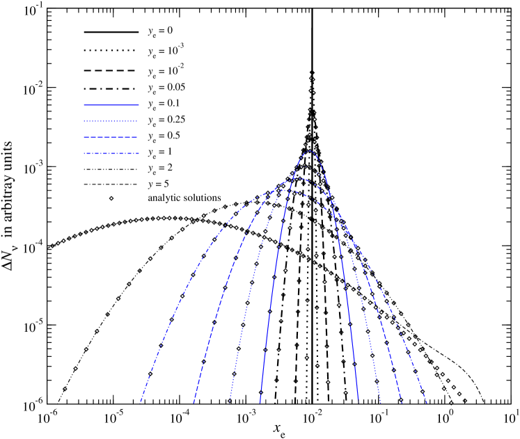
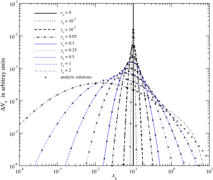
Figure 1: Time-evolution of $\Delta N_{\nu}=\nu^{2}\Delta n$ for different values of the $y$-parameter including the effect of stimulated scattering in the blackbody ambient radiation field. The upper panel shows the case, for an initially narrow line which was injected at frequency $x_{\rm e,0}=10^{-2}$, while the lower panel shows the solution for injection at $x_{\rm e,0}=10^{-1}$. In both figures we show the results as obtained by numerically solving Eq. (12) for $T_{\gamma}=T_{\rm e}$. In addition we give the analytic solutions of the linearized problem, Eq. (13), according to Eq. (14).

Figure 2: Time-evolution of $\Delta N_{\nu}=\nu^{2}\Delta n$ for different values of the $y$-parameter not including the effect of stimulated scattering in the blackbody ambient radiation field (${n_{\rm pl}}=0$). The upper panel shows the case, for an initially narrow line which was injected at $x_{\rm e,0}=10^{-2}$, while the lower panel shows the solution for injection at $x_{\rm e,0}=10^{-1}$. In both figures we show the results as obtained by numerically solving Eq. (12) for $T_{\gamma}=T_{\rm e}$. In addition we give the analytic solutions according to Zeldovich & Sunyaev (1969), Eq. (2).

As an example, in Fig. 1 and 2 we show the time-evolution of an initially narrow line for different values of the $y$-parameter. For the curves shown in Fig. 1 the effect of stimulated scattering in the blackbody ambient radiation field was included, while in Fig 2 it was not. As expected, in the former case the maximum of the distribution is moving toward lower frequencies, while in the latter it moves toward higher frequencies. It is also remarkable that the analytic solution (14) in comparison with the full numerical solution of Eq. (12) works up to values of ${y_{\rm e}}\sim 1-5$. It only breaks down when the photons reach the region $x_{\rm e}\gtrsim 1$, where the recoil effect starts to become important. However, in both considered cases (injection at $x_{\rm e,0}=10^{-2}$ and $x_{\rm e,0}=0.1$) only a small fraction of the initial number of photons reaches this region for ${y_{\rm e}}\lesssim 1$. One can also see that no matter if the background-induced effect is included or not, the line-broadening is not changing much. It is only the position of the line center that is affected by this process, but not the Doppler-broadening.

5 Discussion and conclusion

We have presented a new solution of the Kompaneets-equations for physical situations in which low frequency photons are scattered by thermal electrons but within an intense ambient blackbody field that is very close to full thermodynamic equilibrium with the free electrons. Under these circumstances the blackbody-induced stimulated scattering of photons slows down the motion of photons toward higher frequencies by a factor of $3$ in comparison with the solution that only take into account Doppler-broadening and boosting (Zeldovich & Sunyaev, 1969).

These physical conditions are met during the epoch of cosmological recombination, in particular for ${He\textsc{iii}}\rightarrow{He\textsc{ii}}$-recombination, where electron scattering can still affect the cosmological recombination spectrum notably (Dubrovich & Stolyarov, 1997; Rubino-Martin et al., 2007). The CMB blackbody spectrum is an exact solution of the Kompaneets equation when $T_{\rm e}=T_{\gamma}$. Nevertheless, the weak low frequency features in the presence of CMB with $T_{\rm e}=T_{\gamma}$ are evolving and boosting their central frequencies due to the simultaneous action of induced scattering and Doppler-effect resulting after each scattering. The additional line shift towards low frequencies due to recoil effect is small because $x_{\rm e}\ll 1$.

Since at $z\sim 6000$, i.e. where most of the He ii-photons are released, one finds ${y_{\rm e}}\sim 2\times 10^{-3}$, so that within the standard recombination epoch this process is only important for very accurate predictions of the cosmological recombination spectrum at low frequencies. These may become necessary for the purpose of using the cosmological recombination spectrum for measurements of cosmological parameters, such as the CMB temperature monopole, the specific entropy of the Universe, or the pre-stellar abundance of helium, as discussed recently (Sunyaev & Chluba, 2008). Our analysis shows that the low-frequency spectral features from ${He\textsc{iii}}\rightarrow{He\textsc{ii}}$ recombination should then be shifted by $\Delta\nu/\nu\sim 0.2\%$ instead of $\sim 0.6\%$. At the same time the Doppler-broadening of these lines reaches $\sim 15\%$ at FWHM, and the typical line width is $\Delta\nu/\nu\sim 20-30\%$ (Rubino-Martin et al., 2007).

However, if photons due to uncompensated atomic transitions in hydrogen and helium were released much earlier ($z\gtrsim 10^{4}-10^{5}$) then the blackbody-induced stimulated scattering becomes more significant. As mentioned in the introduction, such emission can occur in connection with possible intrinsic spectral distortions of the CMB, due to energy release in the early Universe (Chluba & Sunyaev, 2008).

We should stress that the discussed behavior of spectral features is characteristic only for the low frequency part of CMB spectrum $h\nu\ll kT_{\gamma}$. In the dm and cm spectral range this condition is fulfilled with very good accuracy, and the occupation number of photons exceeds $\sim 10$. The broadening and shifting of the photons in the Wien-part of the spectrum has completely different behavior and will be discussed in a separate paper.

In addition we gave the solution (6) which describes the evolution of narrow spectral features in the presence of a very bright, broad-band radiation background with ${n_{\rm back}}\gg 1$. It might have interesting applications for radio lines arising inside of extra-galactic radio source. where according to our estimates (see Sect. 3) the background-induced line shifts could be amplified and even exceed the line broadening due to the Doppler-effect.

References

• Arons (1971) Arons, J. 1971, ApJ, 164, 457
• Chluba & Sunyaev (2008) Chluba, J. & Sunyaev, R. A. 2008, ArXiv e-prints, arXiv:0803.3584
• Dubrovich & Stolyarov (1997) Dubrovich, V. K. & Stolyarov, V. A. 1997, Astronomy Letters, 23, 565
• Illarionov & Syunyaev (1972) Illarionov, A. F. & Syunyaev, R. A. 1972, Soviet Astronomy, 16, 45
• Kompaneets (1956) Kompaneets, A. S. 1956, JETP, 31, 876
• Lyubarsky & Sunyaev (1983) Lyubarsky, Y. E. & Sunyaev, R. A. 1983, A&A, 123, 171
• Pozdniakov et al. (1983) Pozdniakov, L. A., Sobol, I. M., & Syunyaev, R. A. 1983, Astrophysics and Space Physics Reviews, 2, 189
• Rubino-Martin et al. (2007) Rubino-Martin, J. A., Chluba, J., & Sunyaev, R. A. 2007, ArXiv e-prints, arXiv:0711.0594
• Sazonov & Sunyaev (2000) Sazonov, S. Y. & Sunyaev, R. A. 2000, ApJ, 543, 28
• Sunyaev (1970) Sunyaev, R. A. 1970, Astrophys. Lett., 7, 19
• Sunyaev & Chluba (2008) Sunyaev, R. A. & Chluba, J. 2008, ArXiv e-prints, arXiv:0802.0772
• Zeldovich & Levich (1968) Zeldovich, Y. B. & Levich, E. V. 1968, Soviet Phys.–JETP, 55, 2423
• Zeldovich & Sunyaev (1969) Zeldovich, Y. B. & Sunyaev, R. A. 1969, Ap&SS, 4, 301