Chiral fermions in a spacetime with multiple warping

Abstract

In a six dimensional brane world model with multiple $S_{1}/Z_{2}$ warping, two of the 4-branes at the boundaries have coordinate dependent brane tensions in order to implement the orbifolded boundary conditions consistently. Such brane tension is shown to be equivalent to a scalar field distribution on the brane dcssg . We show that in such a scenario a masslesss left chiral fermion on the 4-brane localizes naturally on the standard model 3-brane located at one edge of the compact manifold while the massless right chiral fermion wave function as well as the wave functions for the massive fermion modes peak away from this brane. This offers a mechanism of obtaining massless chiral fermion with only one of its chiral component present in our brane.

I Introduction

Warped extra dimensional models have been studied extensively during the last few years ever since Randall and Sundrum proposed the two-brane model to resolve the gauge hierarchy problem in the standard model of elementary particles RS . It has been shown by many that the warped geometries have additional consequences in particle phenomenology and cosmology over and above the hierarchy issue phenom ; horava ; lykken ; cohen ; shiu ; nelson ; chodos ; dienes . Also in recent times several extensions of the RS model have been proposed with more than one extra dimension rshigh . Most of these models consider several independent $S_{1}/Z_{2}$ orbifolds along with a four dimensional Minkowski space-time rshigh .

Recently, Choudhury and SenGupta have proposed an alternative scenario dcssg where the warped compact dimensions get further warped by a series of successive warping leading to multiply warped spacetime with various p-branes sitting at the different orbifold fixed points satisfying appropriate boundary conditions. In this scenario the lower dimensional branes including the standard model 3-brane exist at the intersection edges of the higher dimensional branes. The resulting geometry of the multiply warped D dimensional spacetime is given by : $M^{1,D-1}\rightarrow\left\{[M^{1,3}\times S^{1}/Z_{2}]\times S^{1}/Z_{2}\right\}\times\cdots$, with $(D-4)$ such warped directions. It has been argued that this multiply warped spacetime gives rise to interesting phenomenology and offers a possible explanation of the small mass splitting among the standard model fermions dcssg . One of the interesting characteristics of such a model is the bulk coordinate dependence of the higher dimensional brane tensions. Such a coordinate dependent brane tension is shown to be equivalent to a scalar field distribution on the higher dimensional brane which constitute the bulk for the 3-branes located at the intersection edges of these higher dimensional brane dcssg . While such a scalar field distribution may have several interesting phenomenological significance for the TeV brane Physics, in this work we aim to study the localization issue of the standard model fermions on the visible brane, in particular the occurrence of massless chiral modes of fermions. In the context of the original RS two-brane model it has been shown that fermion localization does take place on the TeV brane and the standard model fermions are confined on the negative tension branechang . For Randall-Sundrum single brane model however one assumes the existence of a bulk scalar field which couples with the bulk fermions ratna . For an appropriate choice for this coupling, one finds that the fermion wave function can be localized on the TeV/standard model brane.

For a six dimensional multiply warped spacetime a scalar field distribution however exists naturally in the form of a coordinate dependent brane tension at the two walls ( 4-branes ). This emerges naturally from the requirement of the orbifolded boundary conditions along the two compact directions dcssg . In this work we first assume that a 6-dimensional bulk fermion is localized on the 4-brane ( i.e the 5D wall) because of the mechanism described in chang . For such five dimensional fermions however no chirality can be defined. These five dimensional fermions can now be further localized on our TeV brane through the naturally occurring coordinate dependent brane tension which is equivalent to a scalar field distribution on the 4-brane. Furthermore for appropriate choice of the coupling parameter between the 5-dimensional fermions and the scalar field distribution only the left chiral mode of the fermion can be localized on our TeV brane while the right handed mode gets more and more localized towards the other 3-brane lying at the other edge of the wallgrossman . Furthermore the massive Kaluza-Klein (KK) modes of the fermion wave functions also tend to peak away from the standard model 3-brane. This phenomena thus offers a natural explanation of the origin of chiral massless fermion mode with only one chiral component in our 3-brane.

The paper is organized as follows. In section II, we discuss about the multiple warped model briefly. Then in section III we focus on the bulk fermions residing on the 4-branes. We examine the localization properties on the standard model 3-brane for the massless modes as well as the massive KK modes originated from the compactification in section IV and V respectively.

II the model

We consider the simplest model of a (5+1) dimensional anti de-Sitter bulk where both the extra dimensions are compactified in succession on circles with $Z_{2}$ orbifoldings. In this set up the solution of the Einstein equation gives rise to a doubly warped spacetime dcssg given by the following metric,

$$ds^{2}=b^{2}(z)[a^{2}(y)\eta_{\mu\nu}dx^{\mu}dx^{\nu}+R^{2}_{y}dy^{2}]+r^{2}_{z}dz^{2}$$ (1)

where the non-compact directions are expressed by $x^{\mu}\,(\mu=0,3)$ and the orbifolded compact directions are denoted by the angular coordinates $y$ and $z$ respectively with $R_{y}$ and $r_{z}$ as respective moduli. Since orbifolding, in general, requires a localized concentration of energy, four 4-branes ($4+1$ dimensional objects) are introduced at the orbifold fixed “points”, namely $y=0,\pi$ and $z=0,\pi$. The total bulk-brane action is given by

$$S=\displaystyle\int{d^{4}x}\,{dy}\,{dz}\,\left[\sqrt{-g_{6}}\;\left(R_{6}-\Lambda\right)+\sqrt{-g_{5}}\left[V_{1}\,\delta(y)+V_{2}\,\delta(y-\pi)\right]\right]$$ (2)

$$+\displaystyle\int{d^{4}x}\,{dy}\,{dz}\,\left[\sqrt{-\widetilde{g}_{5}}\left[V_{3}\,\delta(z)+V_{4}\,\delta(z-\pi)\right]+\sqrt{-g_{vis}}[{\cal L}-\hat{V}]\right]$$

where the brane potential terms are, in general, $V_{1,2}=V_{1,2}(z)$ whereas $V_{3,4}=V_{3,4}(y)$. The corresponding 3-branes are located at $(y,z)=(0,0),(0,\pi),(\pi,0),(\pi,\pi)$. From the above action along with the boundary conditions the exact solution for the bulk metric can be written explicitly in the following form,

$$ds^{2} = \displaystyle\frac{\cosh^{2}(k\,z)}{\cosh^{2}(k\,\pi)}\,\left[\exp\left(-2\,c\,|y|\right)\,\eta_{\mu\nu}\,dx^{\mu}\,dx^{\nu}+R_{y}^{2}\,dy^{2}\right]+r_{z}^{2}\,dz^{2}\$$ (3)

where $k=r_{z}\sqrt{\frac{-\Lambda}{10M^{4}}}$ and $c=\frac{R_{y}k}{r_{z}\cosh(k\pi)}$.

The above solution with doubly orbifolded boundary conditions dcssg results in a box-like picture of the bulk, where the walls of the box are ($4+1$)-dimensional branes. Four ($3+1$) dimensional branes are formed at the four edges of the intersecting 4-branes. Our standard model 3-brane is identified with one of the four edges ( at $y=\pi$, $z=0$ ) by requiring the desired TeV scale while the Planck scale brane resides at another edge. The other two edges correspond to two more $3+1$ dimensional branes with the intermediate energy scales lying very close to TeV for one brane and close to Planck scale for the other. This feature results from a hierarchially different warping in the two compact directions. While warping in one direction is large, the other is necessarily small dcssg .

As discussed earlier that an important feature, relevant for this work in the multiply warped scenario is that the $Z_{2}$ orbifoldings gives rise to coordinate-dependent brane tensions on two 4-branes which are equivalent to a scalar field distribution on the respective branes. Note that in this scenario the coordinate dependent brane tension effectively plays the role of a bulk scalar field which we need not to put in by hand but appears naturally from the requirement of orbifolded boundary conditions along the two internal compact directions. The (4+1) dimensional branes sitting at $y=0$ and $y=\pi$ have the following brane tensions,

$$V_{1}(z)|_{y=0}=8M^{2}\sqrt{\frac{-\Lambda}{10}}~{}{\hbox{sech}}(k\,z)=V_{0}~{}\hbox{sech}(k\,z)=-V_{2}(z)|_{y=\pi}$$ (4)

As the standard model Tev 3-brane is located at $y=\pi$, $z=0$ we are therefore particularly interested in studying the localization of the bulk fermions which are residing on the 4-branes located at $y=\pi$. Note that the 4-brane now defines the bulk for the 3-branes located at (y, z) = ($\pi$, 0) and ($\pi$, $\pi$). It is expected that the coordinate dependent brane tension $V_{2}(z)$ will play an important role in the behavior of the bulk fermions for an appropriate coupling between them.

III Fermion localization

While addressing the issue of fermion localization in a single brane RS model, it was found that one needs to introduce a bulk scalar field to localize fermions on the brane where gravity is localized oda ; kogan . On the contrary in a RS 2-brane model it has been explicitly shown in chang that the exponential warp factor leading to scale hierarchy between the two branes causes the 5D fermions to get localized naturally on the negative tension brane i.e on the TeV brane. Here in the six dimensional model, the warp factor along the $y$ direction is given by the usual RS warp factor $e^{-cy}$. Thus a large warping takes place between the two 4-branes located at $y=0$ and $y=\pi$ leading to the localization of a six dimensional bulk fermion on the 4-brane located at $y=\pi$ which has a negative tension ( just as found in  chang ). However in this case the brane tension being $z$-coordinate dependent (equivalent to a scalar field distribution), we examine the role of such brane tension in localizing the fermion further on the TeV 3-brane ( located at $z=0$ and $y=\pi$) for the two different chiral states.

The metric of the 4+1 dimensional brane at $y=\pi$ is given by

$$ds^{2}=B^{2}(z)[\eta_{\mu\nu}dx^{\mu}dx^{\nu}]+dz^{2}=B_{\pi}^{2}\cosh^{2}(kz)[\eta_{\mu\nu}dx^{\mu}dx^{\nu}]+r^{2}_{z}dz^{2}$$ (5)

where, $B_{\pi}=\frac{exp(-c\pi)}{\cosh(k\pi)}$. The Lagrangian for the Dirac fermions in five-dimensional space-time is given by

$$\sqrt{-g_{5}}{\cal{L}}_{Dirac}=\sqrt{-g_{5}}(\bar{\psi}i\Gamma^{a}D_{a}\psi+\eta\bar{\psi}V_{2}(z)\psi)$$ (6)

where $g_{5}=det(g_{ab})$ is the determinant of the five dimensional metric and $\eta$ measures the strength of the coupling between the fermion and the brane tension. The 4-brane tension $V_{2}(z)$ has been rescaled by $M$ to achieve correct dimensionality. The curved space gamma matrices are represented by $\Gamma^{a}=\left(\frac{1}{B(z)}\gamma^{\mu},-i\gamma^{5}\right)$ where $\gamma^{\mu},\gamma^{5}$ represent four dimensional gamma metrices in chiral representation. The Clifford algebra $\{{\Gamma^{a},\Gamma^{b}}\}=2g^{ab}$ is obeyed by curved gamma metrices. The covariant derivative can be calculated, using the metric and is given by,

$$D_{\mu} = \partial_{\mu}+\frac{1}{2}\Gamma_{\mu}\Gamma^{4}B^{\prime}(z)$$ (7)

$$D_{4} = \partial_{4}$$ (8)

For the above mentioned set up the Dirac Lagrangian turns out to be

$$\sqrt{-g_{5}}{\cal L}_{Dirac}=B^{4}(z)~{}\bar{\psi}\left[\frac{1}{B(z)}i\gamma^{\mu}\partial_{\mu}+\gamma^{5}\left(\partial_{z}+2\frac{B^{\prime}(z)}{B(z)}\right)+\eta V_{2}(z)\right]\psi$$ (9)

Now, the five-dimensional spinor can be decomposed as $\psi(x^{\mu},z)=\psi(x^{\mu})\xi(z)$, where $\psi(x^{\mu})$ is the projection of the 5-dimensional spinor on the 3-brane. In the massless case, we can have definite chiral states viz. $\psi_{L}(x^{\mu})$ and $\psi_{R}(x^{\mu})$ which correspond to left and right chiral states in four dimension. The $\psi_{L}$ and $\psi_{R}$ are given by, $\psi_{L,R}=\frac{1}{2}(1\mp\gamma^{5})\psi$. Here $\xi$ denote the extra dimensional component of the fermion wave function. We then can decompose five-dimensional spinor in the following way liu ,

$$\psi(x^{\mu},z)=\psi_{L}(x^{\mu})\xi_{L}(z)+\psi_{R}(x^{\mu})\xi_{R}(z)$$ (10)

Substituting the above decomposition in the Dirac Lagrangian we obtain the equations for the fermions as,

$$B(z)\left[\partial_{z}+2\frac{B^{\prime}(z)}{B(z)}-\eta V_{2}(z)\right]\xi_{L}(z) = m\xi_{R}(z)$$ (11)

$$B(z)\left[\partial_{z}+2\frac{B^{\prime}(z)}{B(z)}+\eta V_{2}(z)\right]\xi_{R}(z) = -m\xi_{L}(z)$$ (12)

Here we have considered that the four dimensional fermions obey the standard equation of motion, $i\gamma^{\mu}\partial_{\mu}\psi_{L,R}=m\psi_{R,L}$ which in turn implies that the above equations will be obtained provided the following normalization conditions are satisfied:

$$\int^{\pi}_{0}B^{3}(z)~{}\xi^{m}_{L,R}(z)~{}\xi^{n}_{L,R}(z)dz = \delta_{mn}$$ (13)

$$\int^{\pi}_{0}B^{3}(z)~{}\xi_{L}^{m}(z)~{}\xi_{R}^{n}(z)dz = 0$$ (14)

We find it to be interesting to study the localization scenario of both the massless and the massive modes of chiral fermions. After getting the exact solutions of the different modes we discuss about their phemenological implications.

IV Massless modes

We now consider equations (11) and (12) for two different cases namely for zero and non-zero coupling between the bulk fermion and coordinate dependent brane tension.

IV.1 Coupling constant, $\eta=0$

The equations of motion for left and chiral modes become

$$[\partial_{z}+2k\tanh(kz)]\xi_{L,R}(z)=0$$ (15)

The solutions of the above equations are

$$\xi_{L,R}=N_{L,R}~{}{\hbox{sech}}^{2}(kz)$$ (16)

where $N_{L,R}=\left[\frac{k}{2~{}B^{3}_{\pi}~{}\tan^{-1}\tanh(\frac{k\pi}{2})}\right]^{\frac{1}{2}}$ is the normalization constant, found easily from the normalization conditions in (13). Both $\xi_{L,R}$ are peaked at $z=0$, exhibiting the tendency of localization around the 3-brane located at ($\pi$, 0) i.e. on our Standard Model brane irrespective of their chiral states.

Figure 1: Zeromodes are plotted with $k=c=0.1$. Both the left and right chiral modes are peaked at z = 0

However it is apparent from the Figure (1) that the fermion zero modes are not very sharply peaked at the SM brane and have a considerable extension along the extra dimension $z$. Therefore they are not strictly confined on the Tev brane. We shall now see a drastic change in the behavior of the wave function if we switch on the coupling $\eta$.

IV.2 Coupling constant, $\eta\neq 0$

Equations for the left and right chiral modes are given by

$$\left[\partial_{z}+2k\tanh(kz)+\eta V_{0}~{}{\hbox{sech}}(kz)\right]\xi_{L}(z)=0$$ (17)

$$.\left[\partial_{z}+2k\tanh(kz)-\eta V_{0}~{}{\hbox{sech}}(kz)\right]\xi_{R}(z)=0$$ (18)

The solution for the left chiral mode is

$$\xi_{L}(z)=N_{L}~{}{\hbox{sech}}^{2}(kz)~{}\exp\left[-\frac{2\eta V_{0}}{k}\tan^{-1}\left(\tanh\left(\frac{kz}{2}\right)\right)\right]$$ (19)

where $N_{L}=\sqrt{\frac{2\eta V_{0}}{B^{3}_{\pi}\left(1-~{}\exp\left[-\frac{4\eta V_{0}}{k}\tan^{-1}\left(\tanh\left(\frac{k\pi}{2}\right)\right)\right]\right)}}$. Figure (2) shows how the behavior of the left chiral mode varies with increasing values of $\eta$. We find that the these modes become more and more sharply peaked at the brane at $z=0$ as the coupling $\eta$ gets stronger. It may be noted that the maximum value of the function, $\xi^{max}_{L}$, increases with $\eta$ while the position of the maximum always remains fixed at $z=0$.

Figure 2: We have plotted the left chiral modes for $k=c=0.1$ for several values of $\eta$.

To show explicitly the sharpness of the localization of left chiral fermions for strong coupling, we have studied the location of the half value of $\xi^{max}_{L}$ with respect to the point $z=0$, where the peak appears. This is plotted in Figure (3).

Figure 3: Location of the half value of $\xi^{max}_{L}$ is plotted with respect to $\eta$

Note that as $\eta$ increases this location shifts towards the brane at $z=0$. That implies that the left chiral mode is getting more more localized indicating a stronger confinement of the left chiral mode on the standard model brane.

Similarly, the solution for right mode becomes

$$\xi_{R}(z)=N_{R}~{}{\hbox{sech}}^{2}(kz)~{}\exp\left[\frac{2\eta V_{0}}{k}\tan^{-1}\left(\tanh\left(\frac{kz}{2}\right)\right)\right]$$ (20)

where the normalization constant $N_{R}=\sqrt{\frac{2\eta V_{0}}{B^{3}_{\pi}\left(-1+~{}\exp\left[\frac{4\eta V_{0}}{k}\tan^{-1}\left(\tanh\left(\frac{k\pi}{2}\right)\right)\right]\right)}}$. We plot the right chiral modes in the Figure (4).

Figure 4: Right chiral modes are plotted with $k=0.2$ and $c=0.1$ for different values of $\eta$.

From the figure (4) we see that the maximum value of the right mode depends on $\eta$. As $\eta$ increases, the z value at which $\xi_{R}$ becomes maximum shifts away from the brane at $z=0$. Further, as $\eta$ increases, the maximum value of the right mode first decreases with increasing $\eta$ and then it increases. We have shown this in figure (5)

Figure 5: Maximum value of $\xi_{R}$ plotted with respect to $\eta$.

This clearly depicts that with increasing value of $\eta$ the left chiral mode becomes more and more localized on our standard model brane, the right chiral mode on the other hand peaks further away from the SM brane and gets delocalized.

V Massive mode

From the discussion of the massless modes , we have seen that depending on the choice of coupling parameter the left mode gets localized at the SM brane whereas the right mode shifts away from the brane. Of course, when this parameter is zero, both left and right mode solutions become identical and both modes get localized at the SM brane. In this section we turn our attention to the Kaluza-Klein tower of fermions. For an axisymmetric warped brane solution in 6D minimal gauged supergravity it has been shown that the entire KK tower gets localized on the neagtive tension brane param . However, the codimension two defects allow the KK mass gap to remain finite even in the infinite volume limit keeping the modes hidden from present day experiments.

Let us now find out what happens to the massive KK modes in our case. From the equations (11) and (12), using the rescaling $\xi_{L,R}=e^{-5f/2}\tilde{\xi}_{L,R}$, we find that both $\xi_{L}$ and $\xi_{R}$ satisify the same equation which is given as,

$$\tilde{\xi}_{L,R}^{\prime\prime}(z)+\left[-\frac{k^{2}}{4}+\hbox{sech}^{2}(kz)\left(\frac{m^{2}}{B_{\pi}^{2}}-\frac{k^{2}}{4}-\eta^{2}V_{0}^{2}\right)\right]\tilde{\xi}_{L,R}(z)=0$$ (21)

As the massive states are no longer chiral we therefore subesequently drop the indices $L$ and $R$ from the wave function and express it as $\xi(z)$. The equation of the massive modes given in (21) can be reduced to an effective Schrödinger equation problem where the KK modes experience an effective potential having the following form.

$$U_{eff}=-\left(\frac{m^{2}}{B_{\pi}^{2}}-\frac{k^{2}}{4}-\eta^{2}V_{0}^{2}\right)\hbox{sech}^{2}(kz)$$ (22)

Note that the form of the above potential is like the Pösch-Teller potential. The exact solutions of the massive modes can therefore be written as

$${\xi}(z)=\hbox{sech}^{3}(kz)~{}^{2}F_{1}\left[\epsilon-s,\epsilon+s+1,\epsilon+1,\frac{1}{2}(1-\tanh(kz))\right]$$ (23)

where

$$\begin{split}&\epsilon=\frac{1}{2}\\ &s=\frac{1}{2}\left[-1+\frac{1}{k}\sqrt{k^{2}+4\left(\frac{m_{n}^{2}}{B_{\pi}^{2}}-\frac{k^{2}}{4}-\eta^{2}V_{0}^{2}\right)}\right]\end{split}$$ (24)

The mass spectrum can be obtained easily from the requirement that the wave function must be well behaved on the brane. The possible values of the masses for these modes are found to be,

$$m_{n}^{2}={B_{\pi}^{2}}[k^{2}(n^{2}+2n+1)+\eta^{2}V_{0}^{2}]$$ (25)

where n=1,2,3,….
It can be clearly seen from the above expression that the mass squared gap depends linearly on n which is given as,

$$\Delta m_{n}^{2}={B_{\pi}^{2}}k^{2}[2n+3]$$ (26)

Now plugging in the value of ${B_{\pi}^{2}}$ in the above expression and noting that $k$ and $V_{0}$ $\sim M_{P}$, we find $m_{n}\sim$ TeV. Thus all the massive modes have mass of the order of TeV. This apparently raises hope to find signatures of such modes in the forthcoming TeV scale experiments at LHC. To address this issue we now explore whether these massive modes are localized on the SM brane. We draw the behaviour of some wave functions below.

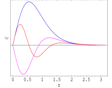
Figure 6: Different modes of massive fermions has been plotted for n = 1, 3 and 5.

It is clearly depicted in Fig.(6) that the wave functions of all such massive fermion modes peak away from the standard model (TeV) brane belying all hopes to find their signature on the TeV brane.

VI conclusion

Extending the earlier work dcssg , where the 4-brane tension for the two branes at $y=0$ and $y=\pi$ were shown to be dependent on the orbifolded co-ordinate $z$, we have shown that such a brane tension actually plays the role of a scalar field distribution and help to localize one of the chiral modes on the TeV 3-brane. Thus one does not need to invoke some external scalar field by hand to achieve the localization. Thus the consistency requirement of the theory itself provides a mechanism for chirality preferential localization. The exact dependence of the wavefunction for the two different chiral modes have been shown with respect to their coupling with the equivalent scalar field distribution originated from the brane tension. It is found that with increasing strength of this coupling we get the desired feature of localization of the left chiral mode on our brane while the right chiral mode peaks away from us. In addition we have also shown that all the massive fermion KK modes have masses of the order of TeV but the wave functions for these massive modes are not localised on the TeV 3-brane making them imperceptible on the TeV brane. This work therefore offers a mechanism to localize only the massless fermions with a definite chirality on the visible 3-brane through multiple warping in a higher dimensional space-time.

- (1) D. Choudhury and S. SenGupta, Phys.Rev. D76, 064030 (2007).
- (2) L. Randall and R. Sundrum, Phys. Rev. Lett. 83, 3370 (1999); ibid Phys. Rev. Lett. 83, 4690 (1999).
- (3) H. Davoudiasl, J. L. Hewett and T. G. Rizzo, Phys. Rev. Lett. 84, 2080 (2000); W. D. Goldberger and M. B. Wise, Phys. Lett. B 475, 275 (2000); H. Davoudiasl and T. G. Rizzo and J. L. Hewett, Phys.Rev. D68, 045002 (2003); C. Csaki, C. Grojean, J. Hubisz, Y. Shirman and J. Terning, Phys. Rev. D 70, 015012 (2004); A. L. Fitzpatrick, J. Kaplan, L. Randall and L. T. Wang, JHEP 0709, 013 (2007)
- (4) R. Dienes, E. Dudas and T. Gherghetta, Phys. Lett.B436, 55 (1998); Z. Kakushadze and S.H.Tye, Nucl. Phys.B548,180 (1999).
- (5) C. Csaki, M. Graesser, C. F. Kolda and J. Terning, Phys. Lett. B 462, 34 (1999); P. Kanti, I. I. Kogan, K. A. Olive and M. Pospelov, Phys. Lett. B 468, 31 (1999); H. Stoica, S. H. H. Tye and I. Wasserman, Phys. Lett. B 482, 205 (2000); N. Chatillon, C. Macesanu and M. Trodden, Phys. Rev. D 74, 124004 (2006); F. Chen, J. M. Cline and S. Kanno, Phys. Rev. D 77, 063531 (2008)
- (6) P. Horava and E. Witten, Nucl. Phys.B475,94,(1996); ibid B460 506 (1996).
- (7) A. Chodos and E. Poppitz, Phys. Lett. B71,119,(1999); T. Gherghetta and M. Shaposhnikov, Phys. Rev. Lett. 85,240,(2000).
- (8) A. G. Cohen and D. B. Kaplan, Phys. Lett. B470 , 52 (1999); I. Antoniadis, S. Dimopoulos and A. Giveon, JHEP, 05, 055 (2001); T. Multamaki and I. Vilja, Phys. Lett. B545, 389 (2002); C. P. Burgess, J. M. Cline, N. R. Constable and H. Firouzjahi, JHEP, 01, 014 (2002).
- (9) C. Csaki and Y. Shirman, Phys. Rev.D61,024008,(2000); A.E. Nelson, Phys. Rev.D63,087503,(2001).
- (10) J. D. Lykken, Phys. Rev. D54, 3693, (1996);J. Lykken and L. Randall, JHEP 06 014 (2000);
- (11) S. Randjbar-Daemi and M.E. Shaposhnikov, Phys.Lett.B491 329 (2000); P. Kanti, R. Madden and K.A. Olive, Phys. Rev. D64 044021 (2001); N.Kaloper, JHEP 0504 061 (2004); T.Gherghetta, A.Kehagias, Phys. Rev. Lett 90 101601 (2003).
- (12) S. Chang, J. Hisano, H. Nakano, N. Okada and M. Yamaguchi, Phys. Rev D62,084025 (2000)
- (13) B. Bajc and G. Gabadadze, Phys. Lett. B474, 282 (2000); I.Oda, Phys.Lett. B496,113 (2000); C. Ringeval, P. Peter and J. P. Uzan, Phys. Rev. D 65, 044016 (2002); R. Koley and S. Kar, Class. Quant. Grav. 22, 753 (2005); ibid Mod. Phys. Lett A20, 363 (2005)
- (14) Y.Grossman and M.Neubert Phys.Lett B474,361-371 (2000)
- (15) Yu-Xiau Liu et. al. hep-th 0803.0098v1(2008); S. Randjbar-Daemi and M. E. Shaposhnikov, Phys. Lett. B492, 361,(2000)
- (16) I. Oda, Phys.Lett. B496, 113,(2000)
- (17) I. I. Kogan, S. Mouslopoulos, A. Papazoglou and G. G. Ross, Nucl. Phys. B 615, 191 (2001)
- (18) S. L. Parameswaran, S. Randjbar-Daemi and A. Salvio, Nucl. Phys. B 767, 54 (2007); S. L. Parameswaran, S. Randjbar-Daemi and A. Salvio, JHEP 0801, 051 (2008)