Observation of Geometric Phases for Three-Level Systems using NMR Interferometry

Abstract

Geometric phase (GP) independent of energy and time rely only on the geometry of state space. It has been argued to have potential fault tolerance and plays an important role in quantum information and quantum computation. We present the first experiment for producing and measuring an Abelian geometric phase shift in a three-level system by using NMR interferometry. In contrast to existing experiments, based on the geometry of $S^{2}$, our experiment concerns the geometric phase with the geometry of $SU(3)/U(2)$. Two interacting qubits have been used to provide such a three-dimensional Hilbert space.

When a quantum mechanical system evolves cyclically in time so that it returns to its initial physical state, its wave function can acquire a geometric phase factor in addition to the familiar dynamic phase 1992Anandan . If the cyclic change of the system is adiabatic, this additional factor is known as Berry’s phase 1984Berry . Otherwise, it is related to Aharonov-Anandan (AA) phase 1987Aharonov that has been pointed out to be a continuous version of earlier Pancharatnam phase 1956Panch .

Geometric phases (GP) independent of energy and time rely only on the geometry of state space. It is therefore resilient to certain types of errors and suggests the possibility of an intrinsically fault-tolerant way of performing quantum gate operations 2000Nielson ; 2000Jones ; 2003Leibfried . This potential value makes it important to observe and further apply GP in different quantum physical systems. The observations of GP began from earlier spin-polarized neutrons through a solenoid 1987Bitter , polarized light through a helically twisted optical fibre 1986Tomita , and a pair of coupled protons in magnetic field using NMR 1989Suter to the recent superconducting qubit experiment 2007Leek . The principle of them are usually the same. That is, in a two-level state space the geometry of it corresponds to a sphere $S^{2}$ and the GP equals to one half the solid angle subtended by closed paths on $S^{2}$.

When one generalizes to a three-level quantum system 1997Khanna ; 1997Arvind , the geometry of $S^{2}$ gets replaced by a four-dimensional geometric space $SU(3)/U(2)$ or part of sphere $S^{7}$. Then evolutions of state correspond to actions of $SU(3)$ on $SU(3)/U(2)$ that is different from that of $SU(2)$ on $S^{2}$ for the two-level case. In order to observe GP, one way to vanish the dynamical phase is closely linked to the geodesic in ray space (see below). For two-level case, the geodesic in ray space happens to coincide with that on $S^{2}$. In contrast, it is a plane curve instead of geodesic on $S^{7}$ for three-level case. The GP for any cyclic evolution in three-level ray space are no longer related to solid angles on $S^{7}$ but referred to Bargmann invariants 1964Bargmann ; 1993Mukunda . All of these differences indicate the observation of three-level GP technically more difficult 2001Sander .

In this letter, we report an experimental observation of three-level GP by using NMR interferometry. The three levels referred in the experiment are chosen from a two spin-$1/2$ interacting system. Unitary evolutions for implementing cyclic paths in the three-dimensional ray space are ensured by quantum controlled logic gate operations 2004Vandersypen . Aimed at obtaining a measurable GP, we evolve the target state while keeping the reference state unchanged to produce a relative phase between them.

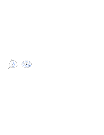
Figure 1: An illustration of the parameter space for all three-level states. The local coordinates $\theta$, $\phi$, $\chi_{1}$ and $\chi_{2}$ are such that $(\theta,\phi)$ define a point in the positive octant of $S^{2}$ and $(\chi_{1},\chi_{2})$ for $(\theta,\phi)$ fixed define a point on a torus.

In the three-dimensional Hilbert space $\mathcal{H}^{3}$, an arbitrary state can be expressed as

$$|\psi\rangle=e^{i\eta}\big{(}e^{i\chi_{1}}\cos\theta,e^{i\chi_{2}}\sin\theta\cos\phi,\sin\theta\sin\phi\big{)},$$ (1)

where the real parameters have the range $\theta,\phi\in[0,\frac{\pi}{2}]$ and $\chi_{1},\chi_{2}\in[0,2\pi)$. It has an one-to-one correspondence, omitting a global phase $\eta$, to the point on an octant of $S^{2}$ plus a torus (Fig. 1). Consider a state evolves from $|\psi(s_{1})\rangle$ to $|\psi(s_{2})\rangle$ with $s_{1,2}$ being the curve parameters determined by the Eq. (1). Corresponding to this evolution, in $\mathcal{H}^{3}$ there is a continuous piecewise smooth parametrized curve, $C=\big{\{}\psi(s)\big{|}s_{1}\leq s\leq s_{2}\big{\}}$, and its image in the ray space $\mathcal{R}$ is likewise continuous and piecewise smooth denoted by $\mathcal{C}=\big{\{}\rho(s)=|\psi(s)\rangle\langle\psi(s)|\big{|}s_{1}\leq s\leq s_{2}\big{\}}$. Then the GP $\beta$ associated with the cure $\mathcal{C}$ equals to the difference between a total phase $\varphi_{\text{tot}}$ and a dynamical phase $\gamma_{d}$ 1997Arvind , that is,

$$\beta[\mathcal{C}] = \varphi_{\text{tot}}[C]-\gamma_{d}[C],$$

$$\varphi_{\text{tot}}[C] = \mathrm{arg}\langle\psi(s_{1})|\psi(s_{2})\rangle,$$ (2)

$$\gamma_{d}[C] = -\int^{s_{2}}_{s_{1}}ds\langle\psi(s)|i\frac{\partial}{\partial s}|\psi(s)\rangle,$$

with both $\varphi_{\text{tot}}$ and $\gamma_{d}$ being functionals of the curve $C$. If the curve $\mathcal{C}$ is closed, the state change can be simply expressed as $|\psi(s_{2})\rangle=\exp\{i(\gamma_{d}[C]+\beta[\mathcal{C}])\}|\psi(s_{1})\rangle$.

The geodesics in ray space $\mathcal{R}$ are given through variations of a nondegenerate positive definite length functional 1993Mukunda . In two-level systems geodesics are related to the parellel transport condition. For the three-level case, every geodesic in ray space has a vanishing geometric phase and it plays a crucial role in the observation of geometric phases in the following. The simplest description of geodesic can always be achieved as follows 1997Arvind . Let $\rho_{k}$ and $\rho_{k+1}$ denote the end points of a smooth curve $\mathcal{C}$ associated with unit vectors $\psi_{k}$ and $\psi_{k+1}$ in $\mathcal{H}^{3}$. There is a requirement for the chosen state vectors that $\langle\psi_{k}|\psi_{k+1}\rangle$ must be real positive. Then the geodesic $\mathcal{C}_{\text{geo}}$ connecting $\rho_{k}$ to $\rho_{k+1}$ is the ray space image of the curve $C_{\text{geo}}=\{\psi(s_{k})|0\leq s_{k}\leq s_{k}^{0}\}$ and

$$\psi(s_{k})=\psi_{k}\cos s_{k}+\frac{\psi_{k+1}-\psi_{k}\langle\psi_{k}|\psi_{k+1}\rangle}{\sqrt{1-\langle\psi_{k}|\psi_{k+1}\rangle^{2}}}\sin s_{k},$$ (3)

with $0\leq s_{k}\leq s_{k}^{0}$ and $s_{k}^{0}=\arccos\langle\psi_{k+1}|\psi_{k}\rangle$. From the Eq. (3), one can see that $\psi(0)=\psi_{k}$ and $|\psi(s_{k}^{0})\rangle\langle\psi(s_{k}^{0})|=|\psi_{k+1}\rangle\langle\psi_{k+1}|=\rho_{k+1}$. For a set of points $\rho_{1},\rho_{2},\cdots,\rho_{n}\subset\mathcal{R}$ in order, suppose that no two consecutive points are mutually orthogonal and that $\rho_{n}$ and $\rho_{1}$ are also nonorthogonal. So we can obtain a closed curve $\mathcal{C}$ in $\mathcal{R}$ in the form of a $n$-sided polygon by joining these $n$ points cyclically with geodesic arcs. The geometric phase is then according to the Eq. (2)

$$\beta[\mathcal{C}] = \mathrm{arg}\langle\psi_{1}|\psi_{1}^{\prime}\rangle-\mathrm{arg}\langle\psi_{1}|\psi_{2}\rangle-\cdots-\mathrm{arg}\langle\psi_{n}|\psi_{1}^{\prime}\rangle$$ (4)

$$= -\mathrm{arg}\mathrm{Tr}(\rho_{1}\rho_{2}\cdots\rho_{n}),$$

in which it has used relations of $|\psi_{1}^{\prime}\rangle\langle\psi_{1}^{\prime}|=|\psi_{1}\rangle\langle\psi_{1}|=\rho_{1}$ and $\rho_{1}^{2}=\rho_{1}$. The Eq. (4) combined with geodesic condition, i.e., $\langle\psi_{k}|\psi_{k+1}\rangle$ is real positive, shows a vanishing dynamical phase for these cyclic evolutions. It thus provides us a convenient evolution way to observe the geometric phase.

Experiments are performed on the three-dimensional subspace of two interacting spin-$\frac{1}{2}$ nuclei—spin $a$ (¹³H) and spin $b$ (¹C) in the ¹³C-labeled chloroform molecule $\mathrm{CHCl_{3}}$. The reduced Hamiltonian for this two spin system is, to an excellent approximation, given by $H=\omega_{a}I^{a}_{z}+\omega_{b}I^{b}_{z}+2\pi JI^{a}_{z}I^{b}_{z}$. The first two terms in the Hamiltonian decribe the free precession of spin a and spin b around the magnetic field $B_{0}$ with Larmour frequencies $\omega_{a}/2\pi\approx 400$ MHz and $\omega_{b}/2\pi\approx 100$ MHz. The third term of the Hamiltonian describes a scalar spin-spin coupling of the two spins with $J=214.5$ Hz. Experiments were performed at room temperature on a Bruker AV-400 spectrometer. If we denote the spin up and down by $|0\rangle$ and $|1\rangle$, the energy levels of such system are displayed in Fig. 2. It has four levels written as $\{|00\rangle,|01\rangle,|10\rangle,|11\rangle\}$ corresponding to energy eigenvalues $\{\frac{1}{2}\hbar(-\omega_{1}-\omega_{2}+\pi J),\frac{1}{2}\hbar(-\omega_{1}+\omega_{2}-\pi J),\frac{1}{2}\hbar(\omega_{1}-\omega_{2}-\pi J),\frac{1}{2}\hbar(\omega_{1}+\omega_{2}+\pi J)\}$. We choose basis states $\{|00\rangle$, $|10\rangle$, $|11\rangle\}$ to construct the desired three-level space $\mathcal{H}^{3}$ and $|01\rangle$ as the reference state which keeps unchanged during evolutions.

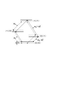
Figure 2: Energy level diagram for (solid lines) two spins coupled by a Hamiltonian of the form of $2\pi\hbar JI_{z}^{1}I_{z}^{2}$ and (dashed lines) two uncoupled spins.

The system was first prepared in a pseudopure state $|00\rangle$ using the method of spatial averaging Cory120 with the pulse sequence

$$R^{b}_{x}(\pi/3)\rightarrow G_{z}\rightarrow R^{b}_{x}(\pi/4)\rightarrow\frac{1}{2J}\rightarrow R^{b}_{y}(\pi/4)\rightarrow G_{z},$$ (5)

which is read from left to right (as the following sequences). The rotations $R^{spins}_{axis}(angle)$ are implemented by radio-frequency pulses. $G_{z}$ is a pulsed field gradient which destroys all coherences (x and y magnetizations) and retains longitudinal magnetization (z magnetization component) only. $\frac{1}{2J}$ represents a free precession period of the specified duration under the coupling Hamiltonian (no resonance offsets).

The complete sequence started by preparing the initial superposition state $\frac{1}{\sqrt{2}}(|00\rangle+|01\rangle)$ with a Hadamard operation on the second qubit of the pseudopure state $|00\rangle$. Then the reference term $|01\rangle$ was kept unchanged through bipartite control operations as shown in Fig. 3. The $|00\rangle$ term (denoted by $|\psi_{1}\rangle$) was first evolved to $|\psi_{2}\rangle=\cos s_{1}^{0}|00\rangle+\sin s_{1}^{0}|10\rangle$ with unitary operation $U_{1}^{\text{g}}(s_{1})$, then to state $|\psi_{3}\rangle=(\cos s_{1}^{0}\cos s_{2}^{0}-e^{i\theta}\sin s_{1}^{0}\sin s_{2}^{0}\cos\varphi)|00\rangle+(\sin s_{1}^{0}\cos s_{2}^{0}+e^{i\theta}\cos s_{1}^{0}\sin s_{2}^{0}\cos\varphi)|10\rangle+\sin\varphi\sin s_{2}^{0}|11\rangle$ with $U_{2}^{\text{g}}(s_{2})$, and last to state $|\psi_{1}^{\prime}\rangle=e^{i\beta}|\psi_{1}\rangle$ with $U_{3}^{\text{g}}(s_{3})$. Corresponding to three smooth geodesics, the unitary operations can be factored into more clear form

$$U_{1}^{\text{g}}(s_{1}) = R(s_{1}),$$

$$U_{2}^{\text{g}}(s_{2}) = R(s_{1}^{0})R_{23}(\theta,\varphi,0)\ R(s_{2})\ R_{23}^{-1}(\theta,\varphi,0)R^{-1}(s_{1}^{0}),$$

$$U_{3}^{\text{g}}(s_{3}) = R_{23}(\chi,\tau,-\xi)\ R(-s_{3})\ R_{23}^{-1}(\chi,\tau,-\xi),$$ (6)

where

$$R(s_{k})=\begin{pmatrix}\cos s_{k}&0&-\sin s_{k}&0\\ 0&1&0&0\\ \sin s_{k}&0&\cos s_{k}&0\\ 0&0&0&1\end{pmatrix},$$

and the $SU(2)_{23}$ subgroup element

$$R_{23}(\theta,\phi,\varphi)=\begin{pmatrix}1&0&0&0\\ 0&1&0&0\\ 0&0&e^{i\phi}\cos\theta&e^{-i\varphi}\sin\theta\\ 0&0&-e^{i\varphi}\sin\theta&e^{-i\phi}\cos\theta\end{pmatrix}.$$

Parameters $\xi,\chi,\tau,s_{3}^{0}$ in Eq. (6) are determined by the reparametrization $|\psi_{3}\rangle=e^{i\xi}\cos s_{3}^{0}|00\rangle+e^{i(\xi+\chi)}\sin s_{3}^{0}\cos\tau|10\rangle+\sin s_{3}^{0}\sin\tau|11\rangle$ and curve parameters $s_{k}$ ($k=1,2,3$) have ranges $0\leq s_{k}\leq s_{k}^{0}$ . Obviously the chosen unit vectors $\psi_{k}$ and $\psi_{k+1}$ satisfy the condition of $\langle\psi_{k}|\psi_{k+1}\rangle$ being real positive. This combined with the Eq. (4) shows a vanishing dynamical phase during these cyclic evolutions and we obtain the GP

$$\beta[\mathcal{C}]=\mathrm{arg}(\cos s_{1}^{0}\cos s_{2}^{0}-e^{i\theta}\sin s_{1}^{0}\sin s_{2}^{0}\cos\varphi).$$ (7)

So after one cyclic evolution described above, it effectively produces a GP and can be measured as a relative phase shift between $|0\rangle_{b}$ and $|1\rangle_{b}$ for the qubit $b$, i.e., $\frac{1}{\sqrt{2}}(|00\rangle+|01\rangle)\rightarrow\frac{1}{\sqrt{2}}(e^{i\beta}|00\rangle+|01\rangle)\rightarrow|0\rangle_{a}\otimes\frac{1}{\sqrt{2}}(e^{i\beta}|0\rangle+|1\rangle)_{b}$. At last the local phase $\beta$ can be read out directly by a phase sensitive detector on qubit $b$ in NMR.

Figure 3: Experimental network: two spin-$1/2$ nuclei perform unitary evolutions controlled by each other. Each circle at the second line means that performs its linked unitary evolution when the second nucleus at $|0\rangle$ state. Each dot at the first line means that performs its linked unitary evolution when the first nucleus at $|1\rangle$ state.

In Fig. 4 we show the measured phase $\beta$ and its dependence on different points $A,B,C$ in ray space characterized by parameters $\{s_{1}^{0},s_{2}^{0},\theta,\varphi\}$, all carried out at $\theta=\pi/4$, and total pulse sequence time $T$ for cyclic evolution is about $5\sim 25ms$ for different evolution path. In Fig. 4 (a) and (b), we set $\varphi=0$ and $\varphi=\pi/4$ respectively with which geodesics have disparate trajectories in ray space. The measured phase is in all cases seen to fit the theoretical curve (7) well with a root-mean-square deviation across all data sets of $5.6$ degree. Thus, all results are in close agreement with the predicted geometric phase, and it is clear that we are able to accurately control the amount of phase geometrically.

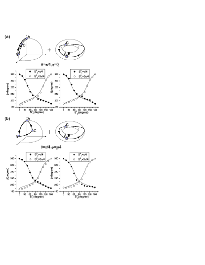
Figure 4: Experimental results on the GP $\beta$ versus the parameter $s_{1}^{0}$ or $s_{2}^{0}$. Changing $s_{1}^{0}$, $s_{2}^{0}$ means changing the positions of the points $B$ and $C$. The evolution paths have been depicted out in parameter space and the theoretical curves are marked out by lines. (a) It shows the result in the case of $\theta=\pi/4$ and $\varphi=0$; the $ABC$ on the octant of $S^{2}$ is a curve while it runs a period on the torus. (b) It shows the result in the case of $\theta=\pi/4$ and $\varphi=\pi/4$; the $ABC$ on the octant of $S^{2}$ is a triangle while it runs a period on the torus.

The controlled operation between the two qubits plays the main role in the experiment. It goes as that the qubit $a$ (or $b$) undergoes a $SU(2)$ operation if the qubit $b$ (or $a$) is in $|1\rangle$ while kept unchanged if it in $|0\rangle$. This is used to realize the controlled operations $R$ and $R_{23}$. The concrete operations go as follows.

For the subsystem of qubit a, we can write the reduced Hamiltonian

$$H_{a}=\omega_{a}I^{a}_{z}+2\pi Jm_{z}^{b}I^{a}_{z}=[\omega_{a}-2\pi J(d^{b}-\frac{1}{2})]I^{a}_{z},$$

where $m_{z}^{b}$ is the eigenvalue of $I_{z}^{b}$ ($=\pm\frac{1}{2}$) and $d^{b}$ the corresponding computational value ($=0,\,1$). If we use a rotating frame with a frequency of $\omega_{a}^{\prime}=\omega_{a}$ and $\omega_{b}^{\prime}=\omega_{b}$, the Hamiltonian turns into, for $d^{b}=0$, $H_{a}^{(0)}=\pi JI^{a}_{z}$, while it becomes $H_{a}^{(1)}=-\pi JI^{a}_{z}$ for $d^{b}=1$. This Hamiltonian generates controlled rotations around the z-axis. To generate the control gate $R(S_{k})$, we rotate the rotation axis using radio-frequency pulses. To generate a $2S_{k}$ rotation around the $y$-axis, e.g., we use the sequence

$$R_{x}^{a}(\frac{\pi}{2})\rightarrow\frac{S_{k}}{\pi J}\rightarrow R_{x}^{a}(-\frac{\pi}{2})\rightarrow R_{y}^{a}(S_{k}).$$

This represents the controlled gate operation $R(S_{k})$.

For another controlled gate operation $R_{23}(\chi,\tau,-\xi)$, we have to reverse the roles of control and target qubit and apply the following sequence to qubit b:

$$R_{z}^{2}(-\phi)\rightarrow R_{y}^{2}(-\pi-\beta)\rightarrow\frac{\alpha}{2\pi J}\rightarrow R_{y}^{2}(\pi+\beta)$$

$$\rightarrow R_{z}^{2}(\phi)\rightarrow R_{n}^{2}(\alpha,\beta,\phi),$$

$R_{n}^{2}(\alpha,\beta,\phi)$ denote to rotate the second qubit $\alpha$ around the axis $\vec{n}(\beta,\phi)$, and $\alpha,\beta,\phi$ is calculated from $\chi,\tau,-\xi$.

In conclusion, when a quantum mechanical system evolves cyclically in time so that it returns to its initial physical state, its wave function can acquire a geometric phase factor in addition to the familiar dynamic phase. Geometric phases (GP) independent of energy and time rely only on the geometry of state space. It is therefore resilient to certain types of errors and suggests the possibility of an intrinsically fault-tolerant way of performing quantum gate operations. we present the first experiment for producing and measuring an Abelian geometric phase shift in a three-level system by using NMR interferometry. In contrast to existing experiments, based on the geometry of $S^{2}$, our experiment concerns the geometric phase with the geometry of $SU(3)/U(2)$. Two interacting qubits have been used to provide such a three-dimensional Hilbert space.

We would like to thank Prof. Zhang for inspiring conversations. This work was supported by the National Natural Science Foundation of China, the CAS, Ministry of Education of PRC, and the National Fundamental Research Program. This work was also supported by European Commission under Contact No. 007065 (Marie Curie Fellowship). J.-L. C. acknowledges supports in part by NSF of China (Grant No. 10575053 and No. 10605013) and Program for New Century Excellent Talents in University.

References

(1)
J. Anandan, The geometric phase. Nature 360, 307-313
(1992).
(2)
M. V. Berry, Proc. R. Soc. A392, 45-57 (1984).
(3)
Y. Aharonov and J. Anandan, Phase Change during a Cyclic
Quantum Evolution. Phys. Rev. Lett. 58, 1593-1596 (1987).
(4)
S. Pancharatnam, Proc. Indian Acad. Sci. A44, 247 (1956).
(5)
M. A. Nielson and I. L. Chuang, Quantum computing and Quantum
Information (Cambridge Univ. Press, Cambridge, 2000).
(6)
J. A. Jones, V. Vedral, A. Ekert, and G. Castagnoli, Geometric
quantum computation using nuclear magnetic resonance. Nature
403, 869-871 (2000).
(7)
D. Leibfried et al., Experimental demonstration of a
robust,high-fidelity geometric two ion-qubit phase gate. Nature
422, 412-415 (2003).
(8)
T. Bitter and D. Dubbers, Manifestation of Berry s
topological phase in neutron spin rotation. Phys. Rev. Lett.
59, 251-254 (1987).
(9)
A. Tomita and R. Y. Chiao, Observation of Berry’s Topological
Phase by Use of an Optical Fiber. Phys. Rev. Lett. 57,
937-940 (1986).
(10)
D. Suter, K. T. Mueller, and A. Pines, Study of the
Aharonov-Anandan Quantum Phase by NMR Interferometry. Phys. Rev.
Lett. 60, 1218 (1988).
(11)
P. J. Leek et al., Observation of Berry’s Phase in a
Solid-State Qubit. Science 318, 1889-1892 (2007).
(12)
L. M. K. Vandersypen and I. L. Chuang, NMR techniques for
quantum control and computation. Rev. Mod. Phys. 76, 1037
(2004).
(13)
G. Khanna, S. Mukhopadhyay, R. Simon, and N. Mukunda,
Geometric Phases for Representations and Three Level
Quantum Systems. Ann. Phys. 253, 55-82 (1997).
(14)
Arvind, K. S. Mallesh, and N. Mukunda, A generalized
Pancharatnam geometric phase formula for three-level quantum
systems. J. Phys. A: Math. Gen. 30, 2417-2431 (1997).
(15)
V. Bargmann, J. Math. Phys. 5 862 (1964).
(16)
N. Mukunda and R. Simon, Quantum Kinematic Approach to the
Geometric Phase. I. General Formalism. Ann. Phys. 228,
205-268 (1993).
(17)
Cory, D. G., Price, M. D. & Havel, T. F. Nuclear magnetic
resonance spectroscopy: An experimentally accessible paradigm for
quantum computing. Phys. D120, 82(1998).
(18)
B. C. Sanders, H. de Guise, S. D. Bartlett, and W. Zhang,
Geometric Phase of Three-Level Systems in Interferometry.
Phys. Rev. Lett. 86, 369-372 (2001).
(19)
M. Reck and A. Zeilinger, Experimental Realization of Any
discrete Unitary Operator. Phys. Rev. Lett. 73, 58-61
(1994).