Narayana numbers and Schur-Szegö composition

Abstract.

In the present paper we find a new interpretation of Narayana polynomials $N_{n}(x)$ which are the generating polynomials for the Narayana numbers $N_{n,k}$ counting Dyck paths of length $n$ and with exactly $k$ peaks, see e.g. [16]. (These numbers appeared recently in a number of different combinatorial situations, [5, 14, 17].) Strangely enough Narayana polynomials also occur as limits as $n\to\infty$ of the sequences of eigenpolynomials of the Schur-Szegö composition map sending $(n-1)$-tuples of polynomials of the form $(x+1)^{n-1}(x+a)$ to their Schur-Szegö product, see below. As a corollary we obtain that every $N_{n}(x)$ has all roots real and non-positive. Additionally, we present an explicit formula for the density and the distribution function of the asymptotic root-counting measure of the polynomial sequence $\{N_{n}(x)\}$.

1. Introduction

1.1. The Narayana numbers, triangle and polynomials

The Narayana numbers $N_{n,k},\;1\leq k\leq n,$ apparently introduced by G. Kreweras in [11] are given by:

$$N_{n,k}=\frac{1}{n}C_{n}^{k-1}C_{n}^{k},$$

where $C_{j}^{i}$ stands for the usual binomial coefficient, i.e. $C_{j}^{i}=\frac{j!}{i!(j-i)!}$.

The latter formula immediately implies that for any fixed $k$ the Narayana numbers $N_{n,k}$ are given by a polynomial in $n$ of degree $2k-2$ divisible by $n$. It is known that $N_{n,k}$ counts, in particular, the number of expressions containing $n$ pairs of parentheses which are correctly matched and which contain exactly $k$ distinct nestings and also the number of Dyck paths of length $n$ with exactly $k$ peaks. (Recall that a Dyck path is a staircase walk from $(0,0)$ to $(n,n)$ that lies strictly above (but may touch) the diagonal $y=x$.) Some other combinatorial interpretations of $N_{n,k}$ can be found in [16] and references therein.

The triangle

$$\begin{array}[]{cccccccccc}&&&&1&&&&\\ &&&1&&1&&&\\ &&1&&3&&1&&\\ &1&&6&&6&&1&\\ 1&&10&&20&&10&&1&\end{array}$$ (1)

of Narayana numbers $N_{n,k}$ read by rows is called the Narayana triangle. (Later we will also interpret this triangle as an infinite lower-triangular matrix taking its left side of ones as the first column and its right side of ones as the main diagonal, see (12).)

The generating functions of the rows of the above triangle are called the Narayana polynomials. More exactly, following the standard convention (see [2]) one defines the $n$-th Narayana polynomial by the formula

$$N_{n}(x)=\sum_{k=1}^{n}N_{n,k}x^{k}~{}~{}.$$

In what follows we will use the following notions. If $P(x)$ is a univariate polynomial of degree $n$, then its reversion or the reverted polynomial $P^{R}(x)$ is defined as $P^{R}(x)=x^{n}P(1/x)$. A polynomial $P(x)$ is called self-reciprocal if it coincides with its revertion up to a sign, i.e. $P(x)=\pm P^{R}(x)$. Hence for any self-reciprocal $P(x)$ if $P(x)$ vanishes at $x_{0}$ then $P(x)$ vanishes at $1/x_{0}$ as well. A polynomial $P(x)$ is called hyperbolic if all its roots are real.

Remark 1.

Each polynomial $N_{n}(x)$ has a simple root at $0$ and each $N_{n}(x)/x$ is self-reciprocal.

The following simple $3$-term recurrence relation satisfied by Narayana polynomials was found in [16, p. 2]:

$$(n+1)N_{n}(x)=(2n-1)(1+x)N_{n-1}(x)-(n-2)(x-1)^{2}N_{n-2}(x),$$ (2)

with the initial conditions $N_{1}(x)=x,\;N_{2}(x)=x^{2}+x$.

1.2. Schur-Szegö composition

The Schur-Szegö composition (CSS) of two degree $n$ polynomials $P=\sum_{j=0}^{n}p_{j}x^{j}$ and $Q=\sum_{j=0}^{n}q_{j}x^{j}$ is defined by the formula:

$$P~{}^{\ast}_{n}~{}Q=\sum_{j=0}^{n}p_{j}q_{j}x^{j}/C_{n}^{j}.$$

When the same $P$ and $Q$ are considered as polynomials of degree $n+k$ with vanishing $k$ leading coefficients then in accordance with the above formula one gets:

$$P~{}^{~{}\,\ast}_{n+k}~{}Q=\sum_{j=0}^{n}p_{j}q_{j}x^{j}/C_{n+k}^{j}.$$

Extending these formulas one defines the composition of $s$ polynomials by the formula:

$$P_{1}~{}^{~{}\,\ast}_{n+k}~{}\cdots~{}^{~{}\,\ast}_{n+k}~{}P_{s}=\sum_{j=0}^{n}p_{1,j}\cdots p_{s,j}x^{j}/(C_{n+k}^{j})^{s-1}~{}.$$

(For more details on CSS see [12, 13].)

Our main goal below will be a further study of a certain linear inhomogeneous map $\Phi_{n}$ initially considered in [9, 1]. Namely, in these papers the first author of the present paper has shown the possibility to present every monic polynomial of degree $n$ with complex coefficients and vanishing at $(-1)$ in the form:

$$P=K_{a_{1}}~{}^{\ast}_{n}~{}\cdots~{}^{\ast}_{n}~{}K_{a_{n-1}}$$ (3)

where each composition factor $K_{a_{i}}$ equals $(x+1)^{n-1}(x+a_{i}),\;a_{i}\in\mathbf{C}.$ (For the sake of convenience, we set $K_{\infty}:=(x+1)^{n-1}$.) Now we can introduce the map $\Phi_{n}$.

Notation 2.

For any $P(x):=(x+1)(x^{n-1}+c_{1}x^{n-2}+\cdots+c_{n-2}x+c_{n-1})$ and for $\nu=1,\ldots,n-1$ set $\sigma_{\nu}:=\sum_{1\leq j_{1}<\cdots<j_{\nu}\leq n-1}a_{j_{1}}\cdots a_{j_{\nu}}$, i.e. define $\sigma_{\nu}$ as the $\nu$-th elementary symmetric function of the roots of the composition factors presenting $P(x)$. Finally, denote by $\Phi_{n}$ the mapping $(c_{1},\ldots,c_{n-1})\mapsto(\sigma_{1},\ldots,\sigma_{n-1})$.

Obviously, $\Phi_{n}$ is linear inhomogeneous. The following theorem was proven in [10].

Theorem 3.

1. The mapping $\Phi_{n}$ has $n-1$ distinct real eigenvalues $\lambda_{1,n}=1$, $\lambda_{2,n}=\frac{n}{n-1}$, $\lambda_{3,n}=\frac{n^{2}}{(n-1)(n-2)}$, $\ldots$, $\lambda_{n-1,n}=\frac{n^{n-2}}{(n-1)!}$.

2. The corresponding eigenvectors are monic polynomials of degree $n-1$ vanishing at $(-1)$ and have the form: $(x+1)^{n-1}$, $x(x+1)^{n-2}$, $x(x+1)^{n-3}Q_{1,n}(x)$, $\ldots$, $x(x+1)Q_{n-3,n}(x)$ where $\deg Q_{j,n}(x)=j$, $j=1,\ldots,n-3$, $Q_{j,n}(-1)\neq 0$. The coefficients of each polynomial $Q_{j,n}(x)$ are rational numbers.

3. Each $Q_{j,n}(x)$ is self-reciprocal. More exactly, $(Q_{j,n}(x))^{R}=(-1)^{j}Q_{j,n}(x)$.

4. The roots of each $Q_{j,n}(x)$, $1\leq j\leq n-3$, are positive and distinct.

5. For $j$ odd (resp. for $j$ even) one has $Q_{j,n}(1)=0$ (resp. $Q_{j,n}(1)\neq 0$). Additionally, the middle coefficient in $(x+1)^{n-j-2}Q_{j,n}(x)$ vanishes if $n$ is even and $j$ is odd.

6. For any $j$ fixed and $n\rightarrow\infty$ the sequence of polynomials $Q_{j,n}(x)$ converges coefficientwise to the monic polynomial $Q_{j}^{*}(x)$ of degree $j$ which has rational coefficients, all roots positive, and satisfies the equality $(Q_{j}^{*}(x))^{R}=(-1)^{j}Q_{j}^{*}(x)$ and the condition $Q_{j}^{*}(1)=0$ for $j$ odd.

Remark 4.

In Theorem 3 we consider the action of $\Phi_{n}$ of the affine $(n-1)$-dimensional space of all monic polynomials of degree $n-1$. If we extend this action to the ambient linear space of all polynomials of degree at most $(n-1)$ then we acquire one more eigenvalue and eigenvector. Namely, the polynomial $(x+1)^{n-2}$ is the eigenvector of $\Phi_{n}$ with the eigenvalue $1$.

1.3. Main results

Set $M_{j}(x)=(-1)^{j-1}xQ_{j-1}^{*}(-x)$. The most important result of the present paper (with a rather lengthy proof) is as follows, see details in Subsection 2.3.

Theorem 5.

For any positive integer $j$ the polynomial $M_{j}(x)$ coincides with the Narayana polynomial $N_{j}(x)$.

Part (6) of the above Theorem 3 then implies the following.

Corollary 6.

Narayana polynomials are hyperbolic for any $n\geq 1$.

More information about the roots of $N_{n}(x)$ is given below. For its proof consult Subsection 2.4.

Theorem 7.

1. The number $(-1)$ is a simple root of $N_{n}(x)$ for any positive even integer $n$. For $n$ odd one has $N_{n}(-1)\neq 0$;

2. All roots of $N_{n}(x)$ are distinct and nonpositive;

3. The roots of $N_{n-1}(x)/x$ interlace with the ones of $N_{n}(x)/x$. Except for the origin the polynomials $N_{n-1}(x)$ and $N_{n}(x)$ have no root in common.

Our final result is as follows, see details in Subsection 2.5. Given a polynomial $P(x)$ of degree $l$ define its root-counting measure $\mu_{P}=\frac{1}{l}\sum_{i=1}^{l}\delta(x-x_{i})$ where $\{x_{1},\ldots,x_{l}\}$ is the set of all roots of $P(x)$ listed with possible repetitions (equal to the respective multiplicities) and $\delta(x-x_{i})$ is the standard Dirac delta-function supported at $x_{i}$. Given a sequence $\{P_{n}(x)\},\deg P_{n}(x)=n,\;n=1,2,\ldots$ we call asymptotic root-counting measure of this sequence the weak limit $\mu=\lim_{n\to\infty}\mu_{P_{n}}$ (if it exists) understood in the sense of distribution theory.

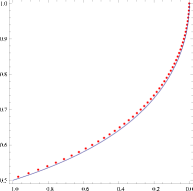
Figure 1. The theoretical distribution $\kappa(x)$ and the empirical distribution of roots of $N_{100}(x)$ on the interval $[-1,0]$.

Theorem 8.

The density $\rho(x)$ and the distribution function $\kappa(x)$ of the asymptotic root-counting measure of the sequence $\{N_{n}(x)\}$ of the Narayana polynomials are given by:

$$\rho(x)=\frac{1}{\pi}\frac{1}{(1-x)\sqrt{-x}};\quad\kappa(x)=1-\frac{2}{\pi}\arctan{\sqrt{-x}},\;x\leq 0.$$ (4)

Remark 9.

Notice that self-reciprocity of $N_{n}(x)$ translates in the following (easily testable) property of $\rho(x)$:

$$x^{2}\rho(x)=\rho\left(\frac{1}{x}\right).$$

Acknowledments. The authors are grateful to Professor Andrei Martinez-Finkelshtein for important conversations. Research of the first author was partially supported by project 20682 of cooperation between CNRS and FAPESP ”Zeros of algebraic polynomials. The second author expresses his gratitude to Laboratoire de Mathématiques, Université de Nice-Sophia-Antipolis for the financial support of his visit to Nice in January 2008.

2. Proofs

2.1. Preliminaries

To prove Theorems 5 and 7 we will need a detailed study of the map $\Phi_{n}$ and, especially, of the equations defining its eigenvectors which in their turn give our polynomials $Q_{j,n}(x)$.

Notation 10.

Set $e_{k}(j)=\sigma_{k}(1,2,\ldots,j)$ to be the value of the $k$-th symmetric function on the $j$-tuple of numbers $(1,2,\ldots,j)$, i.e. $e_{k}(j)=\sum_{1\leq\nu_{1}<\cdots<\nu_{k}\leq j}\nu_{1}\cdots\nu_{k}$, $k=1$, $\ldots$, $j$. Denote by $\phi_{k}(j)$ the sum $1^{k}+2^{k}+\cdots+j^{k}$.

Remark 11.

The quantity $e_{k}(j)$ (resp. $\phi_{k}(j)$) is a polynomial in $j$ of degree $2k$ (resp. of degree $k+1$) divisible by $j(j+1)$.

Let $Q_{j,n}(x):=x^{j}+q_{1}x^{j-1}+\cdots+q_{j-1}x+(-1)^{j}$ be the polynomial introduced in Theorem 3 and set $l_{j}=(n-1)\cdots(n-j)$. Then by (1) of Theorem 3 one has

$$\lambda_{j+2,n}=n^{j+1}/l_{j+1}.$$

(the coefficients $q_{\nu}$ depend also on $j$ and $n$, but we prefer to avoid double indices.) By definition the polynomial $Q_{j,n}(x)$ satisfies the following relation:

$$x(x+1)^{n-j-2}Q_{j,n}(x)=$$

$$=\lambda_{j+2,n}x(x+1)^{n-1}~{}^{\ast}_{n}~{}(x+a_{1})(x+1)^{n-1}~{}^{\ast}_{n}~{}\cdots~{}^{\ast}_{n}~{}(x+a_{j})(x+1)^{n-1}~{}^{\ast}_{n}~{}(x+1)^{n-1},$$

where $\{-a_{1},\ldots,-a_{j}\}$ is the set of all roots of $Q_{j,n}(x)$. After multiplication of both sides of the latter relation by $l_{j+1}$ one gets that the coefficient $R_{k}$ of $x^{k}$, $k\geq 1$, in the right-hand side equals

$$R_{k}:=n^{j+1}C_{n-1}^{k-1}(C_{n-1}^{k}a_{1}+C_{n-1}^{k-1})\cdots(C_{n-1}^{k}a_{j}+C_{n-1}^{k-1})C_{n-1}^{k}/(C_{n}^{k})^{j+1}~{}.$$

The corresponding coefficient $L_{k}$ in the left-hand side equals

$$L_{k}:=(n-1)\cdots(n-j-1)((-1)^{j}C_{n-j-2}^{k-1}+C_{n-j-2}^{k-2}q_{j-1}+\cdots+C_{n-j-2}^{0}q_{j-k+1}).$$ (5)

Therefore one has $q_{\nu}=\sigma_{\nu}$ (see Notation 2) and, finally,

$$R_{k}=n^{j+1}C_{n-1}^{k-1}C_{n-1}^{k}((C_{n-1}^{k-1})^{j}+\sum_{\nu=1}^{j-1}(C_{n-1}^{k-1})^{j-\nu}(C_{n-1}^{k})^{\nu}q_{\nu}+(-1)^{j}(C_{n-1}^{k})^{j})/(C_{n}^{k})^{j+1}.$$ (6)

Thus the coefficients $q_{\nu},\;\nu=1,\ldots,j-1$ of $Q_{j,n}(x)$ solve the system of equations

$$(\Sigma)~{}~{}:~{}~{}\{~{}L_{k}=R_{k}~{},~{}k=1,\ldots,n-1~{}\}.$$ (7)

Lemma 12.

The coefficients $q_{\nu}$ can be expanded in convergent series:

$$q_{\nu}=q_{\nu}^{(0)}+\frac{q_{\nu}^{(1)}}{n-1}+\frac{q_{\nu}^{(2)}}{(n-1)^{2}}+\cdots$$ (8)

with respect to $\frac{1}{n-1}$, where the numbers $q_{\nu}^{(i)}\in{\bf R}$ are uniquely defined and independent of $n$.

Proof: The coefficients $q_{\nu}$ solve system $(\Sigma)$. They are uniquely defined because the polynomials $Q_{j,n}(x)$ are uniquely defined by the eigenvectors of the mapping $\Phi_{n}$. They can be expanded in convergent series in $\frac{1}{n-1}$ because the same property holds for the coefficients of system $(\Sigma)$. As $q_{\nu}$ are uniquely defined, thus $q_{\nu}^{(i)}$ are also uniquely defined.     $\Box$

Remark 13.

We choose to expand $q_{\nu}$ as a series in $\frac{1}{n-1}$ (and not in $\frac{1}{n}$) because the eigenpolynomials of $\Phi_{n}$ (see (2) of Theorem 3) are all of degree $n-1$. Besides, numerical computations show that it is the factor $n-1$ and not $n$ which appears most often in the denominators of the eigenvectors of the mapping $\Phi_{n}$.

Proposition 14.

One has $q_{1}^{(0)}=(-1)^{j}q_{j-1}^{(0)}=-j(j+1)/2$.

Proof: For $k=1$ one has

$$L_{1}=(-1)^{j}(n-1)\cdots(n-j-1)~{}~{},~{}~{}R_{1}=(n-1)(1+\sum_{\nu=1}^{j-1}(n-1)^{\nu}q_{\nu}+(-1)^{j}(n-1)^{j})~{}.$$

The equality $L_{1}=R_{1}$ can be written in the form

$$(-1)^{j}(n-1)\cdots(n-j-1)=(-1)^{j}(n-1)^{j+1}+(n-1)^{j}q_{j-1}^{(0)}+o((n-1)^{j})~{}.$$

Hence $q_{j-1}^{(0)}+o(1)=(-1)^{j}((n-1)\cdots(n-j-1)-(n-1)^{j+1})/(n-1)^{j}$. Observe that

$$(n-1)\cdots(n-j-1)=(n-1)^{j+1}-(1+2+\cdots+j)(n-1)^{j}+o((n-1)^{j})~{}.$$

The quantity $q_{j-1}^{(0)}$ depends on $j$, but not on $n$. Therefore $(-1)^{j}q_{j-1}^{(0)}=-(1+2+\cdots+j)=-j(j+1)/2$.     $\Box$

The next statement is central.

Proposition 15.

1. For each $(\nu,i)$ fixed the coefficient $q_{\nu}^{(i)}$ is given by a real polynomial in $j$ of degree $2(\nu+i)$.

2. For $i=0$ this polynomial is divisible by $j(j+1)$.

2.2. Proof of Proposition 15

$1^{0}$. To prove part (1) of the proposition we use induction on $\nu+i$. Proposition 14 constitutes the base of induction. The step of induction is explained in $2^{0}$ – $3^{0}$.

Recall that the coefficients $q_{\nu}$ give the unique solution to system $(\Sigma)$. From now on we assume that system $(\Sigma)$ is infinite, i.e. $k=1,2,\ldots$. Substituting the expansions (8) of the coefficients $q_{\nu}$ in $(\Sigma)$ we obtain a new system (denoted by $(x)$) with variables $q_{\nu}^{(i)}$, $\nu=1,\ldots,j-1$, $i=0,1,\ldots$. After this substitution the equation $L_{k}=R_{k}$ of system $(\Sigma)$ transforms into an equation of the form $\sum_{l=l_{0}}^{\infty}A_{k,l}/(n-1)^{l}=0$ where the quantities $A_{k,l}$ are some linear inhomogeneous functions of the variables $q_{\nu}^{(i)}$. (Notice that $A_{k,l}$ depend on $j$ but not on $n$.) The latter equation holds for all $n\in{\bf N}$ if and only if all $A_{k,l}$ vanish. (The equation $\{A_{k,l}=0\}$ is denoted by $(A_{k,l})$.)

$2^{0}$. The solution to system $(x)$ is unique (which follows from the uniqueness of the polynomials $Q_{j,n}(x)$ for every fixed $n$, see Theorem 3). This solution depends only on $j$. The self-reciprocity of $Q_{j,n}(x)$ implies that $q_{\nu}^{(i)}=(-1)^{j}q_{j-\nu}^{(i)}$.

In what follows we consider subsystems of system $(x)$ of the form $\{(A_{k,l}),l=l_{0},\ldots,l_{1}\}$, i.e. systems defined in accordance with the filtration of the space of Laurent series in $\frac{1}{n-1}$ by the degree of $\frac{1}{n-1}$. We set $l=s-j-k$.

Notation 16.

Denote by ${\mathcal{I}}_{a,b}$ the set of variables $\{q_{a}^{(0)}$, $q_{a+1}^{(1)}$, $\ldots$, $q_{a+b}^{(b)}\}$.

To settle part (1) of Proposition 15 we need Lemmas 17 and 18 whose proofs are given after that of Proposition 15.

Lemma 17.

The linear inhomogeneous form $A_{k,s-j-k}$ depends only on the variables in the set ${\mathcal{J}}_{j-s,s-1}:={\mathcal{I}}_{j-s,s-1}\cup{\mathcal{I}}_{j-s+1,s-2}\cup\cdots\cup{\mathcal{I}}_{j-1,0}.$

$3^{0}$. Suppose that the variables belonging to the set ${\mathcal{J}}_{j-s+1,s-2}$ are already determined. (For $s=2$ one has ${\mathcal{J}}_{j-s+1,s-2}={\mathcal{I}}_{j-s+1,s-2}={\mathcal{I}}_{j-1,0}=\{q_{j-1}^{(0)}\}$; see Proposition 14.) The system of $s$ linear equations $(A):=\{(A_{k,s-j-k}),k=1,\ldots,s\}$ is a system with $s$ unknown variables, namely, those in the set ${\mathcal{I}}_{j-s,s-1}$. This system has a unique solution (which follows from the existence and uniqueness of the polynomials $Q_{j,n}(x)$, see Theorem 3). Hence the variables in the set ${\mathcal{I}}_{j-s,s-1}$ are uniquely defined.

Lemma 18.

The solution to system $(A)$ is an $s$-vector consisting of real polynomials in $j$ of degree $2s$.

This concludes the proof of the step of induction in part (1) of Proposition 15.

$4^{0}$. For $\nu=1$ part (2) of the proposition follows from Proposition 14. When solving the linear system $(x)$ we express the variables in the set ${\mathcal{I}}_{j-s,s-1}$ as affine functions of the ones in the set ${\mathcal{J}}_{j-s+1,s-2}$. Suppose that all variables in that set are shown to be polynomials divisible by $j(j+1)$. Then the variables in the set ${\mathcal{I}}_{j-s,s-1}$ will be divisible by $j(j+1)$ if and only if this is the case of the constant terms of system $(A)$ (we call them CTs for short).

The CTs are the coefficients of $(n-1)^{s-j-k}$ of the expression $(-1)^{j}U_{1}-U_{2}-(-1)^{j}U_{3}$ where

$$U_{1}=(n-1)\cdots(n-j-1)C_{n-j-2}^{k-1}~{}~{},~{}~{}U_{2}=n^{j+1}C_{n-1}^{k-1}C_{n-1}^{k}(C_{n-1}^{k-1})^{j}~{}~{},$$

$$U_{3}=n^{j+1}C_{n-1}^{k-1}C_{n-1}^{k}(C_{n-1}^{k})^{j}/(C_{n}^{k})^{j+1}~{}~{},$$

see (5) and (6). In this difference the product $U_{2}$ is irrelevant. Indeed, the highest power of $(n-1)$ multiplying any of the variables $q_{\nu}^{(0)}$ in $R_{k}$ is higher than the highest power of $(n-1)$ in $U_{2}$, see (6).

Set $(n-1)\cdots(n-j-1)=(n-1)^{j+1}+V$. Hence $U_{1}=((n-1)^{j+1}+V)C_{n-j-2}^{k-1}$. By Remark 11 the quantity $V$ is a polynomial divisible by $j(j+1)$. Therefore for $j=0$ one has $U_{1}=(n-1)C_{n-2}^{k-1}=nC_{n-1}^{k-1}C_{n-1}^{k}/C_{n}^{k}=U_{3}$, and for $j=-1$ one has $U_{1}=C_{n-1}^{k-1}=U_{3}$. Hence the CTs are divisible by $j(j+1)$. This completes the proof of Proposition 15. Now we settle Lemmas 17 and 18.

Proof of Lemma 17: $1^{0}$. Using the equalities $C_{n-1}^{k-1}/C_{n}^{k}=k/n$ and $C_{n-1}^{k}/C_{n}^{k}=(n-k)/n$, one can present the equality $L_{k}=R_{k}$ (see (5) and (6)) in the form

$$(n-1)\cdots(n-j-1)((-1)^{j}C_{n-j-2}^{k-1}+C_{n-j-2}^{k-2}q_{j-1}+\cdots+C_{n-j-2}^{0}q_{j-k+1})=$$

$$=(n-k)C_{n-1}^{k-1}(k^{j}+\sum_{\nu=1}^{j-1}(n-k)^{\nu}k^{j-\nu}q_{\nu}+(-1)^{j}(n-k)^{j}).$$ (9)

Replace in (9) the quantities $q_{\nu}$ by their expansions (8). Consider the right-hand side $R_{k}$ of (9) as a Laurent series in $\frac{1}{n-1}$. Observe that if the integer $k$ is bounded, then the following relations hold:

$$(n-k)C_{n-1}^{k-1}=\frac{(n-1)^{k}}{k!}+O((n-1)^{k-1})~{}~{},~{}~{}(n-k)^{\nu}k^{j-\nu}=k^{j-\nu}((n-1)^{\nu}+O((n-1)^{\nu-1}).$$

We use the last equality for $\nu=j-s$. The coefficient of $(n-1)^{j-s+k}$ in $R_{k}$ is of the form:

$$\frac{1}{k!}(k^{s}q_{j-s}^{(0)}+k^{s-1}q_{j-s+1}^{(1)}+\cdots+kq_{j-1}^{(s-1)}+{\mathcal{H}}+r),$$

where ${\mathcal{H}}$ is a linear form in the variables $q_{\mu}^{(m)}$ with $\mu-m>j-s$ and $r$ is a real number. Hence the form ${\mathcal{H}}$ contains only variables belonging to the union ${\mathcal{J}}_{j-s+1,s-2}$ (because $\mu\leq j-1$, $m\geq 0$) while the linear form $(1/k!)(k^{s}q_{j-s}^{(0)}+k^{s-1}q_{j-s+1}^{(1)}+\cdots+kq_{j-1}^{(s-1)})$ depends only on the variables in the set ${\mathcal{I}}_{j-s,s-1}$. Hence $R_{k}$ depends only on the variables in the set ${\mathcal{J}}_{j-s,s-1}$.

$2^{0}$. Consider now the left-hand side $L_{k}$ of (9). One can write

$$B(n,j):=(n-1)\cdots(n-j-1)=(n-1)^{j+1}\left(1-\frac{e_{1}(j)}{n-1}+\frac{e_{2}(j)}{(n-1)^{2}}-\cdots\right),$$

see Notation 10. For each $\nu=j-k+1,\ldots,j$ the product $B(n,j)C_{n-j-2}^{\nu-j+k-1}$ is a polynomial in the variable $(n-1)$ of degree $\nu+k$. More precisely,

$$B(n,j)C_{n-j-2}^{\nu-j+k-1}=\frac{(n-1)^{\nu+k}}{(\nu-j+k-1)!}\left(1-\frac{e_{1}(\nu+k-1)}{n-1}+\frac{e_{2}(\nu+k-1)}{(n-1)^{2}}-\cdots\right).$$ (10)

Therefore, the coefficient of $(n-1)^{j-s+k}$ in the term $B(n,j)C_{n-j-2}^{\nu-j+k-1}q_{\nu}$ of $L_{k}$ is of the form

$$\frac{1}{(\nu-j+k-1)!}(q_{\nu}^{(\nu-j+s)}-q_{\nu}^{(\nu-j+s-1)}e_{1}(\nu+k-1)+\cdots+(-1)^{\nu-j+s}q_{\nu}^{(0)}e_{\nu-j+s}(\nu+k-1)).$$ (11)

The index $\nu$ takes the values $j-k+1,\ldots,j-1$, see (9). Hence $L_{k}$ is also a linear inhomogeneous form of the variables in the set ${\mathcal{J}}_{j-s,s-1}$.     $\Box$

Proof of Lemma 18: $1^{0}$. Consider equation $(A_{k,s-j-k})$. Recall that its unknown variables are the ones in the set ${\mathcal{I}}_{j-s,s-1}$. Present this equation in the form $\alpha_{1}q_{j-s}^{(0)}+\cdots+\alpha_{s}q_{j-1}^{(s-1)}=\beta+{\mathcal{G}}$ where the term $\beta$ depends on $j$ but not on the variables $q_{\nu}^{(i)}$ and ${\mathcal{G}}$ is a linear form in the variables $q_{\nu}^{(i)}$ from the set ${\mathcal{J}}_{j-s+1,s-2}$.

$2^{0}$. The quantity $\beta$ is obtained by adding the terms $(n-1)^{j-s+k}$ from the Laurent series of the expressions : $A:=(n-1)\cdots(n-j-1)(-1)^{j}C_{n-j-2}^{k-1}$, $D:=-(n-k)C_{n-1}^{k-1}k^{j}$ and $W:=C_{n-1}^{k-1}(-1)^{j}(n-k)^{j+1}$ in equation (9). The coefficient of $(n-1)^{j-s+k}$ in $A$ equals $(-1)^{j+s}e_{s}(j+k-1)/(k-1)!$ (see equation (10) with $\nu=j$) which is a degree $2s$ polynomial in $j$, see Lemma 11. Its coefficient in $W$ is a polynomial in $j$ of degree $s$. Indeed,

$$W=(-1)^{j}C_{n-1}^{k-1}((n-1)-(k-1))^{j+1}=(-1)^{j}C_{n-1}^{k-1}\sum_{\gamma=0}^{j+1}C_{j+1}^{\gamma}(n-1)^{\gamma}(k-1)^{j+1-\gamma},$$

where $(-1)^{j}C_{n-1}^{k-1}$ is a polynomial in $(n-1)$ of degree $k-1$ and $C_{j+1}^{j-s+1}=C_{j+1}^{s}$ is a polynomial in $j$ of degree $s$. As $k\leq s<j$, there is no term $(n-1)^{j-s+k}$ in $D$. Hence $\beta$ is a polynomial in $j$ of degree $2s$.

$3^{0}$. The linear form ${\mathcal{G}}$ is obtained from certain expressions in both sides of equality (9). First, one considers the terms $B(n,j)C_{n-j-2}^{\nu-j+k-1}q_{\nu}$ in $L_{k}$ and their coefficients of $(n-1)^{j-s+k}$ given by formula (11). Recall that (see Lemma 17) the index $\nu$ takes values $\geq j-s$. Set $\theta:=j-\nu$. Hence $\theta\leq s$. In formula (11) the term $\sigma:=q_{\nu}^{(\delta)}e_{\nu-j+s-\delta}=q_{\nu}^{(\delta)}e_{s-\theta-\delta}$ is the product of the degree $2(s-\theta-\delta)$ polynomial $e_{s-\theta-\delta}$ in the variable $j$ (see Remark 11) and of $\pm q_{j-\nu}^{(\delta)}=\pm q_{\theta}^{(\delta)}$ which is a polynomial of degree $2(\theta+\delta)$ by inductive assumption. Thus $\sigma$ (and, hence, the whole contribution of $L_{k}$ to the linear form ${\mathcal{G}}$) is a polynomial in $j$ of degree $2s$.

$4^{0}$. Secondly, consider in $R_{k}$ the product

$$S:=C_{n-1}^{k-1}(n-k)^{\nu+1}k^{j-\nu}q_{\nu}=C_{n-1}^{k-1}k^{\theta}((n-1)+(1-k))^{\nu+1}\sum_{\eta=0}^{\infty}q_{\nu}^{(\eta)}(n-1)^{-\eta}~{}.$$

The quantity $q_{\nu}^{(\eta)}=\pm q_{\theta}^{(\eta)}$ is a polynomial in $j$ of degree $2(\theta+\eta)$.

Our goal now is to show that the coefficient of $(n-1)^{k+\nu-r}$ in the product $C_{n-1}^{k-1}(n-k)^{\nu+1}$ is a polynomial in $j$ of degree $r$. (We prove this statement in $5^{0}$ below.) This implies that the coefficient of $(n-1)^{j-s+k}$ in $S$ is a finite sum of polynomials in $j$ of degrees $\tau:=2(\theta+\eta)+r$. To obtain a term $(n-1)^{j-s+k}$ we multiply the terms $(n-1)^{k+\nu-r}$ and $(n-1)^{-\eta}$. In other words, one has $(k+\nu-r)-\eta=j-s+k$, i.e. $\nu=j+r+\eta-s$ and $\tau=2(j-\nu+\eta)+r=2s-r<2s$. Thus the contribution of $R_{k}$ to the linear form ${\mathcal{G}}$ is a polynomial in $j$ of degree $<2s$. The lemma is proved.

$5^{0}$. Proof of the latter statement. One has $(n-k)^{\nu+1}=\sum_{r=0}^{\nu+1}C_{\nu+1}^{r}(1-k)^{r}(n-1)^{\nu+1-r}$ and $C_{\nu+1}^{r}$ is a degree $r$ polynomial in $\nu$, and therefore, also in the variable $j-\theta$ and thus in the variable $j$ as well. The binomial coefficient $C_{n-1}^{k-1}$ is a polynomial in $(n-1)$ of degree $(k-1)$ . Thus $C_{n-1}^{k-1}(n-k)^{\nu+1}$ is of the form $\sum_{r=0}^{k+\nu}d_{r}(n-1)^{k+\nu-r}$ where $d_{r}$ is a polynomial in $j$ of degree $r$.     $\Box$

Now we finally return to our main results formulated in the introduction.

2.3. Proof of Theorem 5

$1^{0}$. Consider the lower triangular matrix ${\mathcal{M}}$ whose $j$-th row contains the coefficients of the polynomial $M_{j}(x)$ (starting with the coefficient of the linear term) followed by zeros. Let us turn the Narayana triangle (1) into an infinite lower triangular matrix of the form

$$\mathcal{N}=\begin{pmatrix}1&0&0&0&0&\cdots\\ 1&1&0&0&0&\cdots\\ 1&3&1&0&0&\cdots\\ 1&6&6&1&0&\cdots\\ 1&10&20&10&1&\cdots\\ \vdots&\vdots&\vdots&\vdots&\vdots&\ddots\end{pmatrix}$$ (12)

Theorem 5 claims that the matrices ${\mathcal{M}}$ and ${\mathcal{N}}$ coincide. Denote by ${\mathcal{M}}_{l}$ and ${\mathcal{N}}_{l}$ their $l$-th columns and by ${\mathcal{M}}^{l}$ and ${\mathcal{N}}^{l}$ their $l$-th diagonals (i.e. the sets of entries in positions $(r,r+l-1)$, $r=1,2,\ldots$ in ${\mathcal{M}}$ and ${\mathcal{N}}$ respectively).

The polynomials $M_{j}(x)$ are monic and self-reciprocal with positive coefficients by definition. Therefore, one has ${\mathcal{M}}_{1}={\mathcal{N}}_{1}$, ${\mathcal{M}}^{1}={\mathcal{N}}^{1}$.

$2^{0}$. Suppose that the first $m$ columns (and, hence, the first $m$ diagonals as well) of ${\mathcal{M}}$ coincide with the first $m$ columns (respectively, diagonals) of ${\mathcal{N}}$. The first $m$ entries of ${\mathcal{M}}_{m+1}$ and of ${\mathcal{N}}_{m+1}$ vanish. Their next $m$ entries belong to the first $m$ diagonals, hence, they coincide as well.

$3^{0}$. The entries of ${\mathcal{M}}_{m+1}$ and the ones of ${\mathcal{N}}_{m+1}$ (denoted respectively by ${\mathcal{M}}_{m+1,j}$ and ${\mathcal{N}}_{m+1,j}$) are the values of polynomials $R_{M}^{m+1}$ and $R_{N}^{m+1}$ in $j$ of the same degree $2m$. For ${\mathcal{M}}_{m+1,j}$ this follows from Proposition 15, and for ${\mathcal{N}}_{m+1,j}$ it follows from the next formula for the Narayana numbers:

$$N_{j,m+1}=\frac{1}{j}C_{j}^{m}C_{j}^{m+1}=\frac{(j-1)(j-2)\cdots(j-m+1)}{m!}\frac{j(j-1)\cdots(j-m)}{(m+1)!}.$$ (13)

For $j=1,\ldots,2m$ one has $R_{M}^{m+1}(j)=R_{N}^{m+1}(j)$, see $2^{0}$. For $j=0$ one has $N_{j,m+1}={\mathcal{N}}_{m+1,j}=0={\mathcal{M}}_{m+1,j}$. The first two equalities follow from formula (13), the last one can be deduced from part (2) of Proposition 15. This proposition implies that ${\mathcal{M}}_{m+1,j}$ is divisible by $j(j-1)$ (recall that $M_{j}(x)=(-1)^{j-1}xQ_{j-1}^{*}(-x)$). Hence $R_{M}^{m+1}(x)=R_{N}^{m+1}(x)$.     $\Box$

2.4. Proof of Theorem 7

$1^{0}$. For $n=2$ and $3$ all statements of the theorem can be checked directly. Observe that $N_{n}(x)/x$ has all coefficients positive. By Corollary 6 all roots of $N_{n}(x)/x$ are real, hence negative, and $0$ is a simple root of $N_{n}(x)$.

For any even $n$ it follows from $N_{n}(x)/x$ being self-reciprocal, of odd degree and with positive coefficients that $N_{n}(-1)=0$. For $n$ odd the polynomial $N_{n}(x)$ does not vanish at $(-1)$. This can be proved by induction on $n$. Namely, if $N_{n-2}(x)$ does not vanish at $(-1)$, then the same holds for $N_{n}(x)$, see (2).

$2^{0}$. We prove the rest of the theorem using induction on $n$. Suppose that its statements hold for $N_{2}(x)$, $\ldots$, $N_{n-1}(x)$. Denote by $\xi_{i}$ the $i$-th root of $N_{n-1}(x)$, $\xi_{i}<\xi_{i+1}$, $\xi_{n-1}=0$. By part (3) of the theorem (proved for $N_{n-1}(x)$) one has $N_{n-2}(\xi_{i})/\xi_{i}\neq 0$ and the sign of $N_{n-2}(\xi_{i})/\xi_{i}$ changes alternatively. By equality (2) so does the sign of $N_{n}(\xi_{i})/\xi_{i}$ as well (equality (2) implies that the signs of $N_{n-2}(\xi_{i})/\xi_{i}$ and $N_{n}(\xi_{i})/\xi_{i}$ are opposite). As $N_{n-2}(\xi_{n-2})/\xi_{n-2}>0$, one has $N_{n}(\xi_{n-2})/\xi_{n-2}<0$. The leading coefficient of the polynomial $N_{n}(x)/x$ is positive, hence it has a root in $(\xi_{n-2},0)$ and by self-reciprocity a root in the interval $(-\infty,\xi_{1})$ as well.

The polynomial $N_{n}(x)/x$ is of degree $(n-1)$ and has at least one root in each of the intervals $(-\infty,\xi_{1})$, $(\xi_{1},\xi_{2})$, $\ldots$, $(\xi_{n-2},\xi_{n-1})$. Hence all these roots are simple (including $(-1)$ for $n$ even) and they interlace with the roots of $N_{n-1}(x)/x$. Thus the only root in common for $N_{n}(x)$ and $N_{n-1}(x)$ is $0$ which is simple for both of them, see part 1) of Remark 1.     $\Box$

2.5. On root asymptotics of Narayana polynomials

In this subsection we prove Theorem 8. Define $\Psi_{n}(x)=\frac{N_{n+1}(x)}{N_{n}(x)}$ and $\Theta_{n}(x)=\frac{N_{n}^{\prime}(x)}{nN_{n}(x)},\;n=1,2,\ldots$. Set $\Psi(x)=\lim_{n\to\infty}\Psi_{n}(x)$ and $\Theta(x)=\lim_{n\to\infty}\Theta_{n}(x)$ where these limits exist. $\Psi(x)$ is called the asymptotic quotient and $\Theta(x)$ is called the asymptotic logarithmic derivative of the sequence $\{N_{n}(x)\}$.

Lemma 19.

The sequence $\{\Psi_{n}(x)\}$ of rational functions converges in $\mathbf{C}\setminus\mathbf{R}_{\leq 0}$ to the function $\Psi(x)=x+1+2\sqrt{x}=(\sqrt{x}+1)^{2}$ where $\sqrt{x}$ is the usual branch of the square root which attains positive values for positive $x$. (Here $\mathbf{R}_{\leq 0}$ denotes the half-axis of non-positive numbers.)

Proof of Lemma 19: We need to invoke the classical result of H. Poincaré, see [7, p. 287 - 298] and Theorem 24 and Remark 25 below. Indeed, dividing the recurrence relation (2) by $n+1$ we obtain the normalized reccurence

$$N_{n}(x)-\frac{2n-1}{n+1}(x+1)N_{n-1}(x)+\frac{n-2}{n+1}(x-1)^{2}N_{n-2}(x)=0.$$ (14)

Taking limits of its coefficients when $n\to\infty$ we get from Poincaré’s theorem that the asymptotic quotient $\Psi(x)$ for each $x$ when $\Psi(x)$ exists should satisfy the following quadratic characteristic equation:

$$\Psi^{2}(x)-2(x+1)\Psi+(x-1)^{2}=0.$$ (15)

The exceptional set $E\subset\mathbf{C}$ (called the equimodular discriminant, see [3]) of those values of $x$ for which the equation (15) does not hold consists of all $x$ for which two different solutions $\Psi_{1}(x)$ and $\Psi_{2}(x)$ of (15) have the same absolute value.

Let us show now that in the considered case $E=\mathbf{R}_{\leq 0}$. Indeed, two solutions of (15) are given by $\Psi_{1}(x)=x+1+2\sqrt{x}$ and $\Psi_{2}(x)=x+1-2\sqrt{x}$ for some choice of the branch of square root. One can easily check that if $|\Psi_{1}(x)|=|\Psi_{2}(x)|$ for some value of $x$ then $x+1$ is orthogonal to $\sqrt{x}$ as two vectors in $\mathbf{R}^{2}\simeq\mathbf{C}$. Denoting $\sqrt{x}=A+iB$ one gets $x+1=A^{2}-B^{2}+1+i(2AB)$ and the latter orthogonality condition is given by the relation:

$$A(A^{2}-B^{2}+1)+B(2AB)=0\Longleftrightarrow A(A^{2}+B^{2}+1)=0\Longleftrightarrow A=0.$$

But the real part $A$ of $\sqrt{x}$ vanishes if and only if $x$ is a negative real number implying $E=\mathbf{R}_{\leq 0}$.

Thus the asymptotic quotient $\Psi(x)$ satisfies the equation (15) in $\mathbf{C}\setminus\mathbf{R}_{\leq 0}$. To show that $\Psi(x)=x+1+2\sqrt{x}$, i.e. it chooses the correct branch of solutions to (15) we check that $\Psi(1)=1+1+2=4$ and we prove that $\Psi(x)$ is continuous in $\mathbf{C}\setminus\mathbf{R}_{\leq 0}$.

Indeed, one knows that $N_{n}(1)=\sum_{k=1}^{n}N_{n,k}=Cat_{n}$ where $Cat_{n}=\frac{1}{n+1}\binom{2n}{n}$ is the $n$-th Catalan number, see [16]. Thus $\Psi_{n}(1)=\frac{N_{n+1}(1)}{N_{n}(1)}=\frac{2(n+1)(2n+1)}{(n+2)(n+1)}.$ Therefore, $\Psi(1)=\lim_{n\to\infty}\Psi_{n}(1)=4$. In order to prove the required continuity (and analiticity) we use the well-known Montel’s theorem claiming that a locally bounded family of analytic functions contains a subsequence converging to an analytic function, see e.g [4]. For us it is technically easier to work with the sequence of inverses to $\Psi_{n}(x)$, i.e. with the sequence $\{\frac{N_{n}(x)}{N_{n+1}(x)}\}$. We show that $\{\frac{N_{n}(x)}{N_{n+1}(x)}\}$ is locally bounded in any compact domain separated from $\mathbf{R}_{\leq 0}$. Thus since by Poincaré’s theorem $\{\frac{N_{n}(x)}{N_{n+1}(x)}\}$ is pointwise converging in $\mathbf{C}\setminus\mathbf{R}_{\leq 0}$ one gets by Montel’s theorem that $\{\frac{N_{n}(x)}{N_{n+1}(x)}\}$ converges to an analytic function implying the same fact for the sequence $\{\Psi_{n}(x)\}$. Indeed, by (2) and (3) of Theorem 7 all roots of each $N_{n}(x)/x$ are simple, strictly negative and they interlace with that of $N_{n+1}(x)/x$. Therefore, the partial fractional decomposition of $\frac{N_{n}(x)}{N_{n+1}(x)}$ has the form

$$\frac{N_{n}(x)}{N_{n+1}(x)}=\sum_{i=1}^{n}\frac{\gamma_{i}}{x-a_{i,n+1}},$$

where every $\gamma_{i}$ is positive with $\sum_{i=1}^{n}\gamma_{i}=1$ and $\{a_{1,n+1},\ldots,a_{n,n+1}\}$ is the set of all non-vanishing (and therefore strictly negative) roots of $N_{n+1}(x)$. If $x\in\mathbf{C}$ is any point denote by $\nu(x)$ its Eucledian distance to $\mathbf{R}_{\leq 0}$. Let us check that for any $x\in\mathbf{C}\setminus\mathbf{R}_{\leq 0}$ and for any positive integer $n$ one has

$$\left|\frac{N_{n}(x)}{N_{n+1}(x)}\right|\leq\frac{1}{\nu(x)},$$

which immediately implies the required local boundedness. Indeed,

$$\left|\frac{N_{n}(x)}{N_{n+1}(x)}\right|=\left|\sum_{i=1}^{n}\frac{\gamma_{i}}{x-a_{i,n+1}}\right|\leq\sum_{i=1}^{n}\frac{\gamma_{i}}{|x-a_{i,n+1}|}\leq\sum_{i=1}^{n}\frac{\gamma_{i}}{\nu(x)}=\frac{1}{\nu(x)}.$$

$\Box$

Lemma 20.

The sequence $\{\Theta_{n}(x)\}$ of rational functions converges in $\mathbf{C}\setminus\mathbf{R}_{\leq 0}$ to the function $\Theta(x)=\frac{1}{x+\sqrt{x}}$.

Proof of Lemma 20: Indeed, it is known, see [15], that in case when both the asymptotic quotient $\Psi(x)$ and the asymptotic ratio $\Theta(x)$ exist and have continuous first derivatives in some open domain of $\mathbf{C}$ they satisfy there the relation

$$\Theta(x)=\frac{\Psi^{\prime}(x)}{\Psi(x)}.$$ (16)

A short sketch of its proof is as follows. Consider the difference

$$\frac{\Psi^{\prime}_{n}(x)}{\Psi_{n}(x)}-\Theta_{n}(x)=\frac{p_{n+1}^{\prime}(x)}{p_{n+1}(x)}-\left(1+\frac{1}{n}\right)\frac{p_{n}^{\prime}(x)}{p_{n}(x)}.$$

Then one has,

$$\frac{\Psi^{\prime}(x)}{\Psi(x)}-\Theta(x)=\lim_{n\to\infty}\left(\frac{\Psi^{\prime}_{n}(x)}{\Psi_{n}(x)}-\Theta_{n}(x)\right)=\lim_{n\to\infty}(n+1)\left(\frac{p_{n+1}^{\prime}(x)}{(n+1)p_{n+1}(x)}-\frac{p_{n}^{\prime}(x)}{np_{n}(x)}\right)=0.$$

Applying (16) to the formula for $\Psi(x)$ in Lemma 19 we get

$$\Theta(x)=\frac{\Psi^{\prime}(x)}{\Psi(x)}=\frac{2(\sqrt{x}+1)}{2\sqrt{x}(\sqrt{x}+1)^{2}}=\frac{1}{\sqrt{x}(\sqrt{x}+1)}=\frac{1}{x+\sqrt{x}}.$$

$\Box$

Notation 21.

Given a finite measure $\mu$ supported on $\mathbf{C}$ define its Cauchy transform $\mathcal{C}_{\mu}(x)$ as

$$\mathcal{C}_{\mu}(x)=\int_{\mathbf{C}}\frac{d\mu(\zeta)}{x-\zeta}.$$

The Cauchy transform of the measure is analytic outside its support, its $\frac{\partial}{\partial\bar{z}}$-derivative coincides with the original measure and it has many more important properties, see e.g. [6]. Notice that for any polynomial $P(x)$ of degree $l$ the Cauchy transform $\mathcal{C}_{\mu_{P}}$ of its root-counting measure $\mu_{P}$ is given by the formula $\mathcal{C}_{\mu_{P}}(x)=\frac{P^{\prime}(x)}{l\cdot P(x)}$. Therefore, given a polynomial sequence $\{P_{n}(x)\},\deg P_{n}(x)=n,n=1,2,\ldots$ we have that the Cauchy transform $\mathcal{C}_{\mu}$ of its asymptotic root-counting measure $\mu=\lim_{n\to\infty}\mu_{P_{n}}$ (if the latter measure exists) coincides with the limit $\mathcal{C}_{\mu}(x)=\lim_{n\to\infty}\frac{P_{n}^{\prime}(x)}{nP_{n}(x)}$.

The last result which we need to settle Theorem 8 and which is a particular case of Theorem 3.1.9 of [8] is as follows.

Lemma 22.

If $\rho_{\mu}(x),x\in\mathbf{R}_{\leq 0}$ is the density of a finite measure $\mu$ supported on $\mathbf{R}_{\leq 0}$ and $\mathcal{C}_{\mu}(x),x\in\mathbf{C}\setminus\mathbf{R}_{\leq 0}$ is its Cauchy transform then for any $x\in\mathbf{R}_{\leq 0}$ one has

$$\rho_{\mu}(x)=\frac{i}{2\pi}\left(\overline{\mathcal{C}_{\mu}^{+}(x)-\mathcal{C}_{\mu}^{-}(x)}\right),$$

where $\mathcal{C}_{\mu}^{+}(x)=\lim_{t\to x}\mathcal{C}_{\mu}(x)$ with $t$ belonging to the upper halfplane, $\mathcal{C}_{\mu}^{-}(x)=\lim_{t\to x}\mathcal{C}_{\mu}(x)$ with $t$ belonging to the lower halfplane, and $\overline{Z}$ denotes the usual conjugate of $Z$.

Finally, applying the latter formula to our case we get the required density formula in the statement of Theorem 8. Namely,

$$\rho(x)=\frac{i}{2\pi}\left(\overline{\frac{1}{x+i\sqrt{-x}}-\frac{1}{x-i\sqrt{-x}}}\right)=\frac{i}{2\pi(x^{2}-x)}\left(\overline{(x-i\sqrt{-x})-(x+i\sqrt{-x})}\right)=$$

$$=\frac{i}{2\pi(x^{2}-x)}\cdot\overline{-2i\sqrt{-x}}=\frac{-i^{2}}{\pi}\frac{\sqrt{-x}}{x^{2}-x}=\frac{1}{\pi(1-x)\sqrt{-x}}.$$

Integrating the obtained formula for $\rho(x)$ one gets the expression for the distribution function $\kappa(x)$ from the statement of Theorem 8, see Fig. 1.     $\Box$

3. Appendix. Poincaré’s theorem, [7, p. 287]

1. Set-up. We consider a linear homogeneous difference equation of order $k$

$$f(t+k)+a_{1}f(t+k-1)+a_{2}f(t+k-2)+\cdots+a_{k}f(t)=0$$ (17)

with constant coefficients. Denote by

$$\lambda_{1},\ldots,\lambda_{k}$$

the roots of the characteristic equation

$$\lambda^{k}+a_{1}\lambda^{k-1}+a_{2}\lambda^{k-2}+\cdots+a_{k}=0,$$

and assume that $\lambda_{i}$ have different absolute values denoted by $\xi_{i}=|\lambda_{i}|.$ We can then assume that

$$\xi_{1}>\xi_{2}>\cdots>\xi_{k}.$$ (18)

Since the roots $\lambda_{i}$ are all distinct then the general solution of (17) is given by

$$f(t)=C_{1}\lambda_{1}^{t}+C_{2}\lambda_{2}^{t}+\cdots+C_{k}\lambda_{k}^{t}.$$

Let us choose one single solution of (17), i.e. assign some fixed values to the constants $C_{i}$. Let $C_{p}$ be the first nonvanishing among $C_{i}$’s, i.e.

$$C_{1}=C_{2}=\cdots=C_{p-1}=0\quad{\text{and}}\quad C_{p}\neq 0.$$

Then one can show that

$$\lim_{t\to\infty}\frac{f(t+1)}{f(t)}=\lambda_{p}$$

where $f(t)$ is the considered solution of (17). Indeed, one has

$$\frac{f(t+1)}{f(t)}=\frac{C_{p}\lambda_{p}^{t+1}+C_{p+1}\lambda_{p+1}^{t+1}+\cdots+C_{k}\lambda_{k}^{t+1}}{C_{p}\lambda_{p}^{t}+C_{p+1}\lambda_{p+1}^{t}+\cdots+C_{k}\lambda_{k}^{t}}$$

For $t\to\infty$ one has through (18) that the limits of

$$\left(\frac{\lambda_{p+1}}{\lambda_{p}}\right)^{t},\left(\frac{\lambda_{p+2}}{\lambda_{p}}\right)^{t},\ldots,\left(\frac{\lambda_{k}}{\lambda_{p}}\right)^{t}$$

equal $0$, and we obtain

$$\lim_{t\to\infty}\frac{f(t+1)}{f(t)}=\lambda_{p}$$

that is the following statement is valid

Theorem 23.

If $f(t)$ is an arbitrary (nontrivial) solution of the equation (17) then the limit of the ratio $\frac{f(t+1)}{f(t)}$ for $t\to\infty$ equals one the roots of the characteristic equation if only these roots have distinct absolute values.

We cannot say which root will be involved without the knowledge of the solution. One can only say that this root will have the number $p$ of the first nonvanishing coefficient $C_{p}$ in the considered solution. The following theorem of Poincaré presents a generalization of this statement.

2. Poincaré’s theorem.

Theorem 24.

If the coefficients $P_{i}(t),\;i=0,1,\ldots,k-1$ of a linear homogeneous difference equation

$$f(t+k)+P_{k-1}(t)f(t+k-1)+P_{k-2}(t)f(t+k-2)+\cdots+P_{0}(t)f(t)=0$$ (19)

have limits $\lim_{t\to\infty}P_{i}(t)=a_{i},\;\;i=0,1,\ldots,k-1$ and if the roots of the characteristic equation

$$\lambda^{k}+a_{k-1}\lambda^{k-1}+\cdots+a_{0}=0$$ (20)

have different absolute values then the limit of the ratio $\frac{f(t+1)}{f(t)}$ for $t\to\infty$ of any solution $f(t)$ of the equation (19) equals one of the roots

$$\lambda_{1},\lambda_{2},\ldots,\lambda_{k}$$

of the equation (20), i.e.

$$\lim_{t\to\infty}\frac{f(t+1)}{f(t)}=\lambda_{p}.$$

Remark 25.

In the present paper the role of the quantities $f(t+i)$ is played by the values of the polynomials $N_{n}$ for each $x$ fixed. The parameter $t$ is discrete – this is the index $n$.

References

- [1] [AlKo] S. Alkhatib, V.P. Kostov, The Schur-Szegö composition of real polynomials of degree , Revista Matemática Complutense, to appear.
- [2] [B] P. Barry, On integer-sequence-based constructions of generalized Pascal triangles, J. Integer Sequences, vol. 9 (2006), article 06.2.4.
- [3] [Bi]N. Biggs, Equimodular curves, Discrete Math. 259 (2002) 37–57.
- [4] [Da]K. R. Davidson, Pointwise limits of analytic functions, Amer. Math. Mothly 90(6), (1983) 391–394.
- [5] [DSV] T. Doslic, D. Syrtan, and D. Veljan, Enumerative aspects of secondary structures, Discr. Math., 285 (2004) 67–82.
- [6] [Ga] J. Garnett, Analytic Capacity and Measure. Lect. Notes Math. Vol. 297, Springer-Verlag, iv+138 pp., 1972.
- [7] [Ge] A. O. Gelfond, Differenzrechnung, VEB Deustcher Verlag der Wissenschaften, 1958, 338+vi pp.
- [8] [Hö]L. Hörmander, The analysis of linear partial differential operators. I, Distribution theory and Fourier analysis. Classics in Mathematics, Springer-Verlag, Berlin, 2003.
- [9] [Ko2] V. P. Kostov, The Schur-Szegö composition for hyperbolic polynomials, C.R.A.S. Sér. I 345/9 (2007) 483-488.
- [10] [Ko1] V. P. Kostov, Eigenvectors in the context of the Schur-Szegö composition of polynomials, Mathematica Balkanica, to appear.
- [11] [Kr] G. Kreweras, Sur les éventails de segments, Cahiers du Bureau Universitaire de Recherche Opérationelle, Institut de Statistique, Université de Paris, #15 (1970) 3–41.
- [12] [Pr] V. Prasolov, Polynomials. Translated from the 2001 Russian second edition by Dimitry Leites. Algorithms and Computation in Mathematics, 11. Springer-Verlag, Berlin, 2004, xiv+301 pp. ISBN: 3-540-40714-6.
- [13] [RS] Q.I. Rahman, G. Schmeisser, Analytic Theory of Polynomials, London Math. Soc. Monogr. (N.S.), vol. 26, Oxford Univ. Press, New York, NY, 2002.
- [14] [STT]A. Sapounakis, I. Tasoulas, and P. Tsikouras, Counting strings in Dyck paths, Discr. Math., 307 (2007) 2909–2924.
- [15] [ST] H. Stahl, W. Totik, General orthogonal polynomials, Encyclopedia of Mathematics, Vol. 43, Cambridge Univ. Press, Cambridge, 1992
- [16] [Su] R.A. Sulanke, The Narayana distribution. Special issue on lattice path combinatorics and applications (Vienna, 1998). J. Statist. Plann. Inference 101(1-2), (2002) 311–326.
- [17] [YY] F. Yano, H. Yoshida, Some set partitions statistics in non-crossing partitions and generating functions, Discr. Math. 307 (2007) 3147–3160.