Extended Debye Model for Molecular Magnets

Abstract

Heat capacity data on Mn₁₂ are fitted within the extended Debye model that takes into account a continuum of optical modes as well as three different speeds of sound.

Molecular magnets (MM) such as Mn₁₂ (Ref. T. Lis, 1980) are relatively new materials that have a giant effective molecular spin $S$ (such as $S=10$ for Mn${}_{12})$ built from several atomic spins by a strong intramolecular exchange interaction. The magnetic molecules have a uniaxial anisotropy that is responsible for magnetic bistability and long relaxation over the barrier at low temperatures.R. Sessoli, D. Gatteschi, A. Caneschi, and M. A. Novak (1993) As the magnetic core of these molecules is surrounded by organic ligands, the exchange interaction between different molecules building a crystal lattice is very small. This allows them to relax independently from each other, in contrast to ferromagnets. A fascinating phenomenon discovered in molecular magnets is resonance spin tunneling under the barrier that happens if the energy levels of the spin $S$ in both wells match.J. R. Friedman, M. P. Sarachik, J. Tejada, and R. Ziolo (1996); J. M. Hernández, X. X. Zhang, F. Luis, J. Bartolomé, J. Tejada, and R. Ziolo (1996); L. Thomas, F. Lionti, R. Ballou, D. Gatteschi, R. Sessoli, and B. Barbara (1996)

Molecular magnets is a new type of condensed magnetic systems whose properties differ from those of ferromagnets and dilute paramagnets. Although in the most temperature range MM are paramagnetic, their relaxation can differ from that of a single spin embedded in an elastic matrix. Since the wave length of emitted and absorbed phonons or photons exceeds the lattice spacing, there can be pronounced coherence effects in relaxation such as superradiance. R. Dicke (1954) PhotonE. M. Chudnovsky and D. A. Garanin (2002) and phononE. M. Chudnovsky and D. A. Garanin (2004) superradiance in MM can increase relaxation rates by a huge factor. On the other hand, the opposite effect for initial states of spins with random phases should lead to suppression of the rates by a huge factor. Strong inhomogeneous broadening in MM tends to destroy coherence effects, however, so that efforts should be done to understand the relaxation data. Another collective phenomenon in relaxation that is not yet fully understood theoretically is the phonon bottleneck (see Refs. R. H. Ruby, H. Benoit, and C. D. Jeffries, 1962; A. Abragam and A. Bleaney, 1970 for older reference and Refs. D. A. Garanin, 2007, 2008 for recent work).

To be able to test more sophisticated collective models of relaxation in MM, one should have reliable theoretical estimations of the single-spin relaxation rates, most notably the one-phonon or direct relaxation rate. The latter can depend, in general, on spin-phonon couplings that are difficult to measure. On the other hand, there is a simple mechanism of spin-lattice coupling through rotations of the magnetic molecules by transverse phonons E. M. Chudnovsky (2004); E. M. Chudnovsky, D. A. Garanin, and R. Schilling (2005) that can serve at least as the low bound on spin-lattice relaxation. As in this mechanism the crystal field acting on the spin is not distorted but only rotated, no unknown coupling constants enter the theory. Also this mechanism is likely to be the dominating relaxation channel since the cores of magnetic molecules should be much less deformable than the ligands. The corresponding results for the relaxation rates $\Gamma$ due to direct processes, as well as the Raman processes, depend on only one parameter that is currently not precisely known, the speed of transverse sound $v_{t}$. For direct processes one has $\Gamma\varpropto 1/v_{t}^{5},$ whereas for Raman processes $\Gamma\varpropto 1/v_{t}^{10}.$ Thus the uncertainties of $v_{t}$ dramatically amplify in the relaxation rates.

In the absence of direct measurements of the speed of sound, the latter can be extracted from the heat capacity of the lattice by fitting the measured $C(T)$ to the Debye theory and extracting the Debye temperature $\Theta_{\mathrm{D}}$ that is proportional to the speed of sound. So $\Theta_{\mathrm{D}}=38$ K of Ref. A. M. Gomes, M. A. Novak, R. Sessoli, A. Caneschi, and D. Gatteschi, 1998 results in $v=1600$ m/s, whereas $\Theta_{\mathrm{D}}=41$ K of Ref. F. Fominaya, J. Villain, T. Fournier, P. Gandit, J. Chaussy, A. Fort, A. Caneschi, 1999 results in $v=1727$ m/s. In fact, determination of $\Theta_{\mathrm{D}}$ in Refs. A. M. Gomes, M. A. Novak, R. Sessoli, A. Caneschi, and D. Gatteschi, 1998; F. Fominaya, J. Villain, T. Fournier, P. Gandit, J. Chaussy, A. Fort, A. Caneschi, 1999 relies on the low-temperature data, where the phonon contribution to the heat capacity is $C_{\mathrm{ph}}\varpropto T^{3}$ and the Debye model with the rigid the cut-off at the Brillouin-zone boundary, that is a crude approximation, is not actually used.

A problem with the extracting the Debye temperature and the speed of sound above is the assumption that the three branches of acoustic phonons in the crystal have the same speed $v.$ Indeed, at low temperatures one has $C_{\mathrm{ph}}\varpropto\left(v_{1}^{-3}+v_{2}^{-3}+v_{3}^{-3}\right)T^{3}$, and there is no way to find $v_{i}$ separately from this formula. On the other hand, acoustic phonon modes in such a complicated crystal as Mn₁₂ should not be strictly longitudinal and strictly transverse and all three speeds of sound, as well as all three Debye temperatures, should be different. If they all differ much, the smallest of them dominates the low-temperature heat capacity and, to a much greater extent, the spin-phonon relaxation rates. If one assumes that there are two degenerate transverse phonon modes with $v_{1}=v_{2}=v_{t}\ll v_{3}\equiv v_{l},$ then instead of $\Theta_{\mathrm{D}}=38$ K and $v=1977$ m/s one obtains $\Theta_{\mathrm{D,}t}=33$ K and $v_{t}=1717$ m/s. If there is one phonon mode with $v_{1}\ll v_{2,3},$ then one obtains $\Theta_{\mathrm{D,}1}=26.3$ K and $v_{1}=1368$ m/s.

To improve the description and extract more information, one can use the heat-capacity data at higher temperatures where the contributions from the phonon modes add up in a different way. This is where the Debye model begins to really work and crudeness is introduced into the theory. In addition, optical modes become very important and should be taken into account. In recent Ref. M. Evangelisti, F. Luis, F. L. Mettes, R. Sessoli, and L. J. de Jongh, 2005 on another MM Fe₈ the Debye model has been extended by adding an Einstein oscillator that accounts for all optical modes, and the analysis in a broader temperature range rendered $\Theta_{\mathrm{D}}=19$ K (as well as the Einstein temperature $\Theta_{\mathrm{E}}=38$ K) that differs much from the previousely extracted value $\Theta_{\mathrm{D}}=34$ K for this MM. On the other hand, all three speeds of sound were considered as the same in this analysis.

The data of Ref. A. M. Gomes, M. A. Novak, R. Sessoli, A. Caneschi, and D. Gatteschi, 1998 shown in Fig. 1 go as $C\varpropto T$ at elevated temperatures, and the heat capacity per molecule by far exceeds the value $3k_{\mathrm{B}}$ of a crystal with one atom per unit cell at $T\gtrsim\Theta_{\mathrm{D}}$. This means that there are a lot of optical modes forming a continuum with a nearly constant density of states. This is expected for molecular magnets having hundreds of atoms within the unit cell. Description based on a continuum of optical modes is much more reasonable than the Einstein theory with all due respect. The aim of the present paper is thus to formulate the extended Debye model (EDM) including a continuum of optical modes. This will be used to extract the speeds of sound in Mn₁₂ from the experimental data without making the assumption $v_{1}=v_{2}=v_{3}.$

\begin{picture}(11.0,5.5)\centerline{\hbox{\psfig{angle=-90,width=227.62204pt}}} \end{picture}

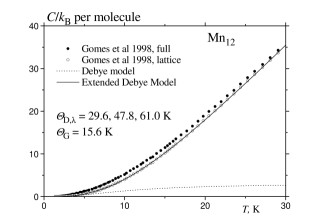
Figure 1: Heat capacity of Mn${}_{12}.$ The standard Debye model fails everywhere except for very low temperatures, while the extended Debye model perfectly fits the data.

The thermal energy of acoustic phonons per unit cell of a crystal is given by

$$U_{\mathrm{ph}}=\frac{1}{N}\sum_{\mathbf{k}\lambda}\frac{\hbar\omega_{\mathbf{k}\lambda}}{\exp\left(\frac{\hbar\omega_{\mathbf{k}\lambda}}{k_{\mathrm{B}}T}\right)-1},$$ (1)

where $N$ is the number of unit cells in the crystal, $\omega_{\mathbf{k}\lambda}$ are phonon frequencies and $\lambda=1,2,3$ are phonon polarizations. One can replace summation over $\mathbf{k}$ by integration. Within the Debye model one assumes that the relation $\omega_{\mathbf{k}\lambda}=v_{\lambda}k$ holds everywhere in the Brillouin zone that is approximated by a sphere bound by the Debye wave vector $k_{\mathrm{D}}.$ The latter is defined by the requirement that that total number of phonon modes is $N:$

$$1=\frac{1}{N}\sum_{\mathbf{k}}=v_{0}\int_{0}^{k_{D}}\frac{4\pi k^{2}dk}{\left(2\pi\right)^{3}}=v_{0}\frac{k_{\mathrm{D}}^{3}}{6\pi^{2}},$$ (2)

where $v_{0}$ is the unit-cell volume. This yields

$$k_{\mathrm{D}}=\left(6\pi^{2}/v_{0}\right)^{1/3}.$$ (3)

One can introduce Debye frequencies $\Omega_{\mathrm{D},\lambda}$ and Debye temperatures $\Theta_{\mathrm{D},\lambda}$ for different acoustic phonon branches $\lambda$ as

$$\Omega_{\mathrm{D},\lambda}=v_{\lambda}k_{\mathrm{D}},\qquad k_{\mathrm{B}}\Theta_{\mathrm{D},\lambda}=\hbar\Omega_{\mathrm{D},\lambda}.$$ (4)

Now Eq. (1) can be written as

$$U_{\mathrm{ph}}=\sum_{\lambda}\int d\omega\rho_{\lambda}(\omega)\frac{\hbar\omega}{\exp\left(\frac{\hbar\omega}{k_{\mathrm{B}}T}\right)-1},$$ (5)

where the densities of states are given by

$$\rho_{\lambda}(\omega)=3\omega^{2}/\Omega_{\mathrm{D},\lambda}^{3}$$ (6)

for $\omega<\Omega_{\mathrm{D},\lambda}$ and zero otherwise. At low temperatures, $T\ll\Theta_{\mathrm{D}},$ Eq. (5) yields

$$U_{\mathrm{ph}}=k_{\mathrm{B}}\frac{\pi^{4}}{5}\sum_{\lambda}\frac{T^{4}}{\Theta_{\mathrm{D},\lambda}^{3}}.$$ (7)

and thus

$$C_{\mathrm{ph}}=\frac{dU_{\mathrm{ph}}}{dT}=k_{\mathrm{B}}\frac{4\pi^{4}}{5}\sum_{\lambda}\frac{T^{3}}{\Theta_{\mathrm{D},\lambda}^{3}}.$$ (8)

At high temperatures, $T\gg\Theta_{\mathrm{D}},$ Eq. (5) yields

$$U_{\mathrm{ph}}=3k_{\mathrm{B}}T,\qquad C_{\mathrm{ph}}=3k_{\mathrm{B}}.$$ (9)

For all $\Theta_{\mathrm{D},\lambda}$ being the same, the coefficient in Eq. (8) is a huge number $12\pi^{4}/5\simeq 234.$ Because of this, Eq. (8) does not smoothly join with Eq. (9) at $T\sim\Theta_{\mathrm{D}}$, and the applicability of Eqs. (7) and (8) requires in fact very low temperatures, not just $T\ll\Theta_{\mathrm{D}}.$ On the other hand, Eq. (9) is at striking contradiction with the experiments shown in Fig. 1 because of the huge unaccounted contribution of optical modes. Thus the usefulness of the Debye model in its standard form is limited, at least for molecular magnets.

To improve the Debye model in a minimal way, one can add optical modes with a constant density of states

$$\rho_{\lambda}(\omega)=3/\Omega_{\mathrm{G}},\qquad\omega\geq\Omega_{\mathrm{D},\lambda}$$ (10)

where $\Omega_{\mathrm{G}}$ is another characteristic frequency that should be considered as a fitting parameter. With Eqs. (6) and (10) inserted, Eq. (5) becomes

$$\frac{U_{\mathrm{ph}}}{k_{\mathrm{B}}} = 3\sum_{\lambda}\frac{T^{4}}{\Theta_{\mathrm{D},\lambda}^{3}}F_{3}\left(\frac{\Theta_{\mathrm{D},\lambda}}{T}\right)$$ (11)

$$-\frac{3T^{2}}{\Theta_{\mathrm{G}}}\sum_{\lambda}F_{1}\left(\frac{\Theta_{\mathrm{D},\lambda}}{T}\right)+\frac{3}{2}\pi^{2}\frac{T^{2}}{\Theta_{\mathrm{G}}},$$

where $k_{\mathrm{B}}\Theta_{\mathrm{G}}=\hbar\Omega_{\mathrm{G}}$ and

$$F_{n}\left(y\right)\equiv\int_{0}^{y}dx\frac{x^{n}}{e^{x}-1}.$$ (12)

For the heat capacity one obtains

$$\frac{C_{\mathrm{ph}}}{k_{\mathrm{B}}} = 12\sum_{\lambda}\frac{T^{3}}{\Theta_{\mathrm{D},\lambda}^{3}}F_{3}\left(\frac{\Theta_{\mathrm{D},\lambda}}{T}\right)-\frac{6T}{\Theta_{\mathrm{G}}}\sum_{\lambda}F_{1}\left(\frac{\Theta_{\mathrm{D},\lambda}}{T}\right)$$ (13)

$$+3\sum_{\lambda}\left(\frac{\Theta_{\mathrm{D},\lambda}}{\Theta_{\mathrm{G}}}-1\right)\frac{\Theta_{\mathrm{D},\lambda}/T}{e^{\Theta_{\mathrm{D},\lambda}/T}-1}+3\pi^{2}\frac{T}{\Theta_{\mathrm{G}}}.$$

In the high-temperature limit $T\gg\Theta_{\mathrm{D}}$ these equations yield

$$U_{\mathrm{ph}}=\frac{3}{2}\pi^{2}k_{\mathrm{B}}\frac{T^{2}}{\Theta_{\mathrm{G}}},\qquad C_{\mathrm{ph}}=3\pi^{2}k_{\mathrm{B}}\frac{T}{\Theta_{\mathrm{G}}},$$ (14)

instead of Eq. (9) and in accord with the experimental data of Ref. A. M. Gomes, M. A. Novak, R. Sessoli, A. Caneschi, and D. Gatteschi, 1998 shown in Fig. 1.

\begin{picture}(11.0,5.5)\centerline{\hbox{\psfig{angle=-90,width=227.62204pt}}} \end{picture}

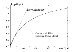
Figure 2: Heat capacity of Mn₁₂ in $C(T)/T$ vs $T^{2}$ representation used to eliminate the small parasite term $C(T)\varpropto T$.

\begin{picture}(11.0,5.5)\centerline{\hbox{\psfig{angle=-90,width=227.62204pt}}} \end{picture}

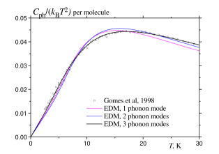
Figure 3: Heat capacity of Mn₁₂ in the presentation used as a crucial test for different models. One can see that only the model with three different acoustic phonon modes fits the data.

To fit the experimental heat capacity with Eq. (13), one has first to subtract the spin (Schottky) contribution $C_{S}(T)$ from $C(T).$ Using the spin Hamiltonian in zero field

$$\hat{H}=-DS_{z}^{2}-AS_{z}^{4}+\hat{H}^{\prime},$$ (15)

where $D/k_{\mathrm{B}}=0.548$ K, $A/k_{\mathrm{B}}=1.1\times 10^{-3}$ K, I. Mirebeau, M. Hennion, H. Casalta, H. Andres, H. U. Güdel, A. V. Irodova, and A. Caneschi (1999); E. del Barco, A. D. Kent, E. M. Rumberger, D. N. Hendrickson, and G. Cristou (2003) and $\hat{H}^{\prime}$ is the part of the Hamiltonian that does not commute with $S_{z},$ nonessential for $C_{S}(T)$ in Mn${}_{12}.$ With the spin levels $\varepsilon_{m}=-Dm^{2}-Am^{4}$ the energy is given by $U_{S}=\left(1/Z\right)\sum_{m=-S}^{S}\varepsilon_{m}\exp\left[-\varepsilon_{m}/\left(k_{\mathrm{B}}T\right)\right],$ where $Z=\sum_{m=-S}^{S}\exp\left[-\varepsilon_{m}/\left(k_{\mathrm{B}}T\right)\right].$ Then $C_{S}=dU_{S}/dT,$ and fitting the lattice heat capacity $C_{\mathrm{ph}}=C-C_{S}$ yields the EDM curve shown in Fig. 1 that is in an excellent accord with the experimental data in the entire temperature range.

In fact, the lattice heat capacity also contains the contribution of nuclear spins $\sim 1/T$ that is small in the Kelvin range, as well as the $T$-linear term that must be an artefact of the experimental procedure. To eliminate the parasite $T$-term and visualize the $C_{\mathrm{ph}}\varpropto T^{3}$ dependence at low temperatures, it is convenient to plot $C_{\mathrm{ph}}/T$  vs $T^{2}$ to get a straight line, as shown in Fig. 2. The slope of the straight line yields the average value of the Debye temperature $\bar{\Theta}_{\mathrm{D}}\equiv\left(\sum_{\lambda}\Theta_{\mathrm{D},\lambda}^{-3}/3\right)^{-1/3}=38$ K, in accord with Ref. A. M. Gomes, M. A. Novak, R. Sessoli, A. Caneschi, and D. Gatteschi, 1998, whereas the coefficient in the $T$-linear term is 0.022. Subtracting this small constant and fitting the rest, one obtains

$$\Theta_{\mathrm{D},1}=29.6\ \text{K,\quad}\Theta_{\mathrm{D},2}=47.8\ \text{K,\quad}\Theta_{\mathrm{D},3}=61.0\ \text{K,}$$ (16)

as well as

$$\Theta_{\mathrm{G}}=15.6\ \text{K.}$$ (17)

From Eqs. (4) and (16) follows

$$v_{1}=1541\ \text{m/s,\quad}v_{2}=2488\ \text{m/s,\quad}v_{3}=3176\ \text{m/s.}$$ (18)

The first of these speeds of sound should correspond to a nearly transverse mode, while the last one should correspond to a nearly longitudinal mode. The former is the most important in relaxation.

Of course, one can say that with enough fitting parameters one can fit any function. While in general it is true, the scheme used here is a minimal model with no excessive fitting parameters. Accounting for optical phonons with a single parameter $\Theta_{\mathrm{G}}$ is a must, and there are no physical reasons to set speeds of sound the same. The experimental results in the natural representation in Fig. 1 can also be fitted by the EDM with one acoustic phonon mode ($v_{1}=v_{2}=v_{3}=v$) and two acoustic phonon modes ($v_{1}=v_{2}=v_{t},$ $v_{3}=v_{l}$), and the results are visually not dramatically worse. However, this fitting method is inferior since it puts more weight on the high-temperature range and tends to neglect the low-temperature range. It is better to fit the $C/T$ data with the subtraction of the parasite $T$-term, as was done above (see Fig. 2). Then one can see more difference between different fits. The most stringent check of different fits can be achieved in the most balanced representation of $C(T)$ over the whole temperature range using $C/T^{2}$ (with subtracted $T$-term) as the fitting target. The results shown in Fig. 3 demonstrate that only the model with three different speeds of sound really fits the data. In addition, for this model results obtained with different fitting methods do not differ much. Fitting of $C/T^{2}$ with three phonon modes yields $\Theta_{\mathrm{D},\lambda}=29.7,$ 47.1, 61.4 K and $\Theta_{\mathrm{G}}=15.7\$K that is very close to the results of the $C/T$ fitting, Eqs. (16) and (17), and even to the results of the $C$ fitting ($\Theta_{\mathrm{D},\lambda}=29.5,$ 50.0, 57.0 K and $\Theta_{\mathrm{G}}=15.8\$K). To the contrary, models with one or two different speeds of sound yield very different results with the three different fitting schemes. Thus one concludes that these models do not work. Still we quote the results from fitting $C/T^{2}$ in Fig. 3 for the reference: One phonon mode $\Theta_{\mathrm{D}}=39.4$ K and $\Theta_{\mathrm{G}}=18.4\$K, two phonon modes $\Theta_{\mathrm{D},t}=38.1$ K, $\Theta_{\mathrm{D},l}=41.3$ K, and $\Theta_{\mathrm{G}}=17.5\$K.

\begin{picture}(11.0,5.5)\centerline{\hbox{\psfig{angle=-90,width=227.62204pt}}} \end{picture}

Figure 4: Phonon density of states for Mn₁₂ within the extended Debye model.

Fig. 4 shows the density of states in Mn₁₂ within the extended Debye model with parameters given by Eqs. (16) and (17). Although there are steps in the DOS that reflect the crudeness of the underlying Debye model, there are three smaller steps instead of a single large step in the original Debye model. Thus the EDM is much more realistic than the DM. The accuracy of the extracted data on speeds of sound is difficult to estimate because of the assumption of the rigid cut-off at $k_{\mathrm{D}}.$ One rather should consider Eqs. (16)–(18) as qualitative results that capture some physics of phonons in MM.

A practical question is how to apply the results obtained above to the relaxation in MM. All existing formulas are based on the model with one longitudinal phonon mode and two transverse phonon modes. Within the mechanism of the molecule rotation without distortion, the contributions of the processes contain the factors $\sin^{2}\theta=\left[\mathbf{k\times e}_{\mathbf{k}\lambda}\right]^{2}/k^{2},$ where $\mathbf{e}_{\mathbf{k}\lambda}$ are phonon polarization vectors. Thus longitudinal phonons do not make a contribution while transverse phonons make the maximal contribution. In reality phonons are not purely longitudinal and purely transverse and it is difficult to extract the angle between $\mathbf{k}$ and $\mathbf{e}_{\mathbf{k}\lambda}.$ For an estimation one can propose a rule of thumb: $\theta=\pi/2,$ $\pi/4,0$ for the phonon modes with $v_{1},$ $v_{2},$ and $v_{3},$ respectively. With this conjecture, one can make the following replacement in the formulas for the rates of direct processes:

$$\frac{1}{v_{t}^{5}}\Rightarrow\frac{1}{2}\left(\frac{1}{v_{1}^{5}}+\frac{1/2}{v_{2}^{5}}\right)=\frac{1}{2v_{1}^{5}}\left[1+\frac{1}{2}\left(\frac{v_{1}}{v_{2}}\right)^{5}\right].$$ (19)

For the values listed in Eq. (18), the correction term in square brackets is only 0.046 and can be neglected. Thus the rule of thumb simplifies to keeping only the softest mode with the coefficient 1/2. Then the increase of the rate due to using the model with three different phonon modes instead of the traditional model with one longitudinal and two degenerate transverse phonon modes is given by $v_{t}^{5}/(2v_{1}^{5})=\Theta_{\mathrm{D},t}^{5}/(2\Theta_{\mathrm{D},1}^{5}).$ With $\Theta_{\mathrm{D},1}=29.7$ and $\Theta_{\mathrm{D},t}=38.1$ K obtained above, the rate increase makes up $\Theta_{\mathrm{D},t}^{5}/(2\Theta_{\mathrm{D},1}^{5})=2.4.$

The author thanks Marco Evangelisti for providing many illuminating insights into the low-temperature heat capacity measurements, Jonathan Friedman for stimulating this research, and Eugene Chudnovsky for useful discussions. This work has been supported by the NSF Grant No. DMR-0703639.

References

- (1)
- T. Lis (1980) T. Lis, Acta Crystallogr. B 36, 2042 (1980).
- R. Sessoli, D. Gatteschi, A. Caneschi, and M. A. Novak (1993) R. Sessoli, D. Gatteschi, A. Caneschi, and M. A. Novak, Nature (London) 365, 141 (1993).
- J. R. Friedman, M. P. Sarachik, J. Tejada, and R. Ziolo (1996) J. R. Friedman, M. P. Sarachik, J. Tejada, and R. Ziolo, Phys. Rev. Lett. 76, 3830 (1996).
- J. M. Hernández, X. X. Zhang, F. Luis, J. Bartolomé, J. Tejada, and R. Ziolo (1996) J. M. Hernández, X. X. Zhang, F. Luis, J. Bartolomé, J. Tejada, and R. Ziolo, Europhys. Lett. 35, 301 (1996).
- L. Thomas, F. Lionti, R. Ballou, D. Gatteschi, R. Sessoli, and B. Barbara (1996) L. Thomas, F. Lionti, R. Ballou, D. Gatteschi, R. Sessoli, and B. Barbara, Nature 383, 145 (1996).
- R. Dicke (1954) R. Dicke, Phys. Rev. 93, 99 (1954).
- E. M. Chudnovsky and D. A. Garanin (2002) E. M. Chudnovsky and D. A. Garanin, Phys. Rev. Lett. 89, 157201 (2002).
- E. M. Chudnovsky and D. A. Garanin (2004) E. M. Chudnovsky and D. A. Garanin, Phys. Rev. Lett. 93, 257205 (2004).
- R. H. Ruby, H. Benoit, and C. D. Jeffries (1962) R. H. Ruby, H. Benoit, and C. D. Jeffries, Phys. Rev. 127, 32 (1962).
- A. Abragam and A. Bleaney (1970) A. Abragam and A. Bleaney, Electron Paramagnetic Resonance of Transition Ions (Clarendon Press, Oxford, 1970).
- D. A. Garanin (2007) D. A. Garanin, Phys. Rev. B 75, 094409 (2007).
- D. A. Garanin (2008) D. A. Garanin, Phys. Rev. B 77, 024429 (2008).
- E. M. Chudnovsky (2004) E. M. Chudnovsky, Phys. Rev. Lett. 92, 120405 (2004).
- E. M. Chudnovsky, D. A. Garanin, and R. Schilling (2005) E. M. Chudnovsky, D. A. Garanin, and R. Schilling, Phys. Rev. B 72, 94426 (2005).
- A. M. Gomes, M. A. Novak, R. Sessoli, A. Caneschi, and D. Gatteschi (1998) A. M. Gomes, M. A. Novak, R. Sessoli, A. Caneschi, and D. Gatteschi, Phys. Rev. B 57, 5021 (1998).
- F. Fominaya, J. Villain, T. Fournier, P. Gandit, J. Chaussy, A. Fort, A. Caneschi (1999) F. Fominaya, J. Villain, T. Fournier, P. Gandit, J. Chaussy, A. Fort, A. Caneschi, Phys. Rev. B 59, 519 (1999).
- M. Evangelisti, F. Luis, F. L. Mettes, R. Sessoli, and L. J. de Jongh (2005) M. Evangelisti, F. Luis, F. L. Mettes, R. Sessoli, and L. J. de Jongh, Phys. Rev. Lett. 95, 227206 (2005).
- E. del Barco, A. D. Kent, E. M. Rumberger, D. N. Hendrickson, and G. Cristou (2003) E. del Barco, A. D. Kent, E. M. Rumberger, D. N. Hendrickson, and G. Cristou, Phys. Rev. Lett. 91, 047203 (2003).
- I. Mirebeau, M. Hennion, H. Casalta, H. Andres, H. U. Güdel, A. V. Irodova, and A. Caneschi (1999) I. Mirebeau, M. Hennion, H. Casalta, H. Andres, H. U. Güdel, A. V. Irodova, and A. Caneschi, Phys. Rev. Lett. 83, 628 (1999).