Strictly and asymptotically scale-invariant probabilistic models of $N$ correlated binary random variables having q–Gaussians as $N\to\infty$ limiting distributions

Abstract

The celebrated Leibnitz triangle has a remarkable property, namely that each of its elements equals the sum of its South-West and South-East neighbors. In probabilistic terms, this corresponds to a specific form of correlation of $N$ equally probable binary variables which satisfy scale-invariance. Indeed, the marginal probabilities of the $N$-system precisely coincide with the joint probabilities of the $(N-1)$-system. On the other hand, the nonadditive entropy $S_{q}\equiv\frac{1-\int_{-\infty}^{\infty}[p(x)]^{q}}{q-1}$ $(q\in{\mathbb{R}};\,S_{1}=-\int_{-\infty}^{\infty}p(x)\ln p(x))$, which grounds nonextensive statistical mechanics, is, under appropriate constraints, extremized by the ($q$–Gaussian) distribution $p_{q}(x)\propto[1-(1-q)\,\beta\,x^{2}]^{1/(1-q)}$ ($q<3$; $p_{1}(x)\propto e^{-\beta x^{2}})$. These distributions also result, as attractors, from a generalized central limit theorem for random variables which have a finite generalized variance, and are correlated in a specific way called $q$–independence. In order to physically enlighten this concept, we introduce here three types of asymptotically scale-invariant probabilistic models with binary random variables, namely (i) a family, characterized by an index $\nu=1,2,3,\dots$, unifying the Leibnitz triangle ($\nu=1$) and the case of independent variables ($\nu\to\infty$); (ii) two slightly different discretizations of $q$–Gaussians; (iii) a special family, characterized by the parameter $\chi$, which generalizes the usual case of independent variables (recovered for $\chi=1/2$). Models (i) and (iii) are in fact strictly scale-invariant. For models (i), we analytically show that the $N\to\infty$ probability distribution is a $q$–Gaussian with $q=(\nu-2)/(\nu-1)$. Models (ii) approach $q$–Gaussians by construction, and we numerically show that they do so with asymptotic scale-invariance. Models (iii), like two other strictly scale-invariant models recently discussed by Hilhorst and Schehr (2007), approach instead limiting distributions which are not $q$–Gaussians. The scenario which emerges is that asymptotic (or even strict) scale-invariance is not sufficient but it might be necessary for having strict (or asymptotic) $q$–independence, which, in turn, mandates $q$–Gaussian attractors.

I INTRODUCTION

The central limit theorem (CLT) provides a most powerful tool to explain the ubiquity of Gaussian distributions in physical systems. It explains that $N$ independent or weakly correlated arbitrarily distributed random variables, with finite variances, sum up to Gaussian probability distributions for $N\to\infty$, corresponding to the thermodynamical limit in physical systems. This theorem constitutes part of the foundations of Boltzmann-Gibbs (BG) statistical mechanics, making it possible to describe a vast number of systems without accounting for the specific micro-dynamics constituting them.

On the other hand, in systems dominated by strongly correlated microscopic events, correlations have remained a stumbling block for the researcher, making it extremely difficult to adequately take into account the contribution of all the microscopic events in order to get a general macroscopic behavior.

Recently, specific generalizations of the CLT have been proposed taking into account some classes of global correlations, typically correlations over long distances Tsallis:05 ; Umarov:08 ; Umarov:06a ; Umarov:07 ; UmarovTsallis2007 ; UmarovTsallis2008 ; UmarovQueiros2008 ; TsallisQueiros2007 ; QueirosTsallis2007 . Let us briefly review the present situation. When we have $N$ identical independent random variables whose individual distribution has a finite variance, their sum approaches, as $N$ diverges and after appropriate centering and scaling, a Gaussian distribution. This is the so-called standard CLT. If the individual variance diverges (due to fat tails of the power-law class, excepting for possible logarithmic corrections), the attractor is a Lévy distribution (also called sometimes $\alpha$-stable distribution). If the variables are not independent but $q$–independent (the $q=1$ particular instance recovers standard probabilistic independence), then, if certain $q$–generalized variance is finite, the attractor is a $q$–Gaussian distribution Umarov:08 ; if that variance diverges (due to specific power-law asymptotics), then the attractor is a $(q,\alpha)$-stable distribution Umarov:06a . These various results have been numerically illustrated in TsallisQueiros2007 ; QueirosTsallis2007 , and some extensions can be seen in Umarov:07 ; UmarovTsallis2007 ; UmarovTsallis2008 ; UmarovQueiros2008 ; Vignat:07 . When $q=1$, the correlations disappear, and the $q$–Gaussian ($(q,\alpha)$-stable distribution) reproduces a Gaussian (Lévy distribution). In terms of mathematical grounding of statistical mechanics, the $q\neq 1$ CLT cases play for nonextensive statistical mechanics Tsallis:88 ; next:04 ; next:05 ; biblio the same role that the $q=1$ CLT cases play for the BG theory. The development of this theory is motivated by the observation that $q$-Gaussians (or distributions very close to them) appear in many real physical systems, such as cold atoms in dissipative optical lattices Douglas2006 , dusty plasma Goree2008 , motion of Hydra cells Upaddhyaya:01 , and defect turbulence Daniels:04 . This suggests that this kind of probability distribution plays an important role in system out-of equilibrium presenting global correlations.

A central point of this generalized theorem is of course the hypothesis of $q$–independence (defined in Umarov:08 through the $q$–product Nivanen:03 ; Borges:04 , and the $q$–generalized Fourier transform Umarov:08 ). This corresponds, when $q\neq 1$, to a global correlation of the $N$ random variables. Its rigorous definition is however not transparent enough in physical terms. An important goal along these lines is therefore to describe in simple terms the basic physical assumptions behind the mathematical requirement of $q$–independence. Two types of simple models have been recently introduced MoyanoGellmann:2006 ; Thistleton:06 in order to provide this insight. They are hereafter referred to as the MTG and the TMNT models respectively. The first one is a discrete model with binary random variables; the second one involves continuous variables. They both are strictly scale-invariant and have been found numerically to converge, when $N$ increases, on distributions remarkably close to $q$–Gaussians. However, a rigorous analytical treatment showed that the functional form of the probability distribution, although being amazingly well fitted by $q$–Gaussians in both models, differs from it in the thermodynamical limit Hilhorst:07 . This fact established that strict scale-invariance (hence asymptotic-scale invariance) is not sufficient for having $q$–Gaussians as limiting distributions. It remained open the question whether scale-invariance allows for such limiting distributions. In the present paper, we precisely clarify this central issue, thus providing some insight into this problem.

After some brief review of the theoretical frame within which $q$–Gaussians emerge, we introduce, in Sec. III, a strictly scale-invariant family of Leibnitz–like triangles, for which the limiting distribution can be exactly obtained. Its limiting distributions are $q$–Gaussians, which proves that scale-invariance is consistent with $q$–Gaussianity. In Sec. IV we discretize (in two slightly different manners) $q$–Gaussians. We then show numerically that these discretized distributions approach the limiting ones —$q$–Gaussians by construction— with asymptotic scale-invariance. This illustrates that both strict and asymptotic scale-invariances are compatible with $q$–Gaussianity. Finally, in Sec. V we introduce another family of strictly scale-invariant probabilistic triangles which, like the MTG and TMNT models, do not converge onto $q$–Gaussians, but onto rather curious distributions, having a singular behavior at infinity. We conclude in Sec. VI.

II $q$–GAUSSIANS

In addition to their appearance in a $q$–generalized CLT, $q$–Gaussians are the nonextensive statistical mechanical Tsallis:88 ; next:04 ; next:05 ; biblio analog to Gaussians in the BG theory. By introducing a generalized entropic functional, a generalized thermostatistics could be developed that exhibits a thermodynamic scenario similar to that of the original one. This theory accounts for a class of systems where the BG theory fails. The entropy $S_{q}$ (with $q\neq 1$) was proposed as an alternative to the BG entropy for complex systems, e.g., trapped in nonergodic non–equilibrium states Pluchino:07 ; Pluchino:08 , or nonlinear dynamical systems at the edge of chaos Tirnakli:07 ; Tirnakli:08 . Also, a connection between this generalized entropy and the generalized nonlinear Fokker-Planck equation leading to anomalous diffusion has been established Bukman:96 .

Indeed, $p_{1}(x)\propto e^{-x^{2}/2\sigma^{2}}$ optimizes the BG entropy $S_{1}=-k\int_{-\infty}^{\infty}p_{1}(x)\ln p_{1}(x)\,dx$, under constraints $\int_{-\infty}^{\infty}dx\,p_{1}(x)=1$ and $\langle x^{2}\rangle_{1}\equiv\int_{-\infty}^{\infty}dx\,x^{2}p_{1}(x)=\sigma^{2}$. Analogously, $q$–Gaussians

$$p_{q}(x)\propto\left[1-(1-q)\beta x^{2}\right]^{\frac{1}{1-q}}~{}~{}~{}~{}~{}(q<3)$$ (1)

optimize the entropy

$$S_{q}[p_{q}(x)]=k\dfrac{1-\displaystyle\int_{-\infty}^{\infty}dx\,\left[p_{q}(x)\right]^{q}}{q-1}$$

under constraints $\int_{-\infty}^{\infty}dx\,p_{q}(x)=1$ and Prato:99

$$\langle x^{2}\rangle_{q}\equiv\dfrac{\displaystyle\int_{-\infty}^{\infty}dx\,x^{2}[p_{q}(x)]^{q}}{\displaystyle\int_{-\infty}^{\infty}dx\,[p_{q}(x)]^{q}}=\sigma^{2}$$

It must be noted that $q$–Gaussians (1) have compact support ($|x|\leqslant 1/\sqrt{(1-q)\beta}$) for $q<1$ and are defined for all $x$ for $q\geqslant 1$. In addition, the second moment of $q$–Gaussians remains finite for $q<5/3$. In the following, we will consider $\beta=1$. The distribution $P_{q}(x)\equiv[p_{q}(x)]^{q}/\int_{-\infty}^{\infty}dx\,[p_{q}(x)]^{q}$ is called escort distribution escort and its relevance is discussed, for instance, in TsallisPlastinoAlvarez2008 . $S_{q}$ is nonadditive for $q\neq 1$ since, for two independent systems $A$ and $B$, we easily verify (assuming $k=1$) $S_{q}(A+B)=S_{q}(A)+S_{q}(B)+(1-q)S_{q}(A)S_{q}(B)$.

In complex cases, the BG entropy generally looses its extensivity, i.e., it no more (asymptotically) increases linearly with the system size. In this paper, the emphasis is to consider $q$–Gaussians as being limiting probability functions characteristic for non-equilibrium states. We will determine the characteristic entropic index for the simple systems described in the following sections but do not necessarily expect them to yield extensivity of the $q$–entropy with the same value for $q$ that they exhibit in the stationary state distribution.

III FIRST MODEL: A FAMILY OF LEIBNITZ-LIKE TRIANGLES

In a probabilistic context, scale invariance will be said to (strictly) occur when, for a set of $N$ random variables, the functional form of the associated marginal probabilities of the $N$-variables set coincides with the joint probabilities associated with the $(N-1)$-variables set, i.e, when

$$\int p_{N}(x_{1},x_{2},\dots,x_{N-1},x_{N})\,dx_{N}=p_{N-1}(x_{1},x_{2},\dots,x_{N-1})~{}.$$ (2)

This relation is always valid for independent random variables, where the joint probability corresponds to the product of the individual probabilities, but it is by no means necessarily valid for correlated ones (see, for instance, Sec. IV for a counter example).

We take now the case of a set of binary independent variables, each one taking values 1 or 0 with probabilities $p$ and $1-p$ respectively. For $N=2$, the joint and marginal probability distributions are given by Table 1.

$x_{1}\backslash^{\displaystyle x_{2}}$	1	0
1	$p^{2}$	$p(1-p)$	$p$
0	$p(1-p)$	$(1-p)^{2}$	$1-p$
	$p$	$1-p$	1

Table 1: Joint probability distribution for a set of $N=2$ independent binary variables.

Last row (column) of Table 1 represents the marginal probabilities of $x_{2}$ ($x_{1}$) which reproduce the form of the probability distribution for each single ($N=1$) variable. For the $N=3$ case, it is necessary to project a cube in the plane in order to represent the whole set of probabilities (Table 2).

${x_{1}\backslash^{\displaystyle x_{2}}}^{\displaystyle\backslash^{\displaystyle x_{3}}}$	1	0
1	$p^{3}$	$p^{2}(1-p)$
	$[p^{2}(1-p)]$	$[p(1-p)^{2}]$
0	$p^{2}(1-p)$	$p(1-p)^{2}$
	$[p(1-p)^{2}]$	$[(1-p)^{3}]$

Table 2: Joint probability distribution for a set of $N=3$ independent binary variables.

Each box of Table 2 contains two probabilities. The one in brackets stands for the case $x_{3}=0$, the other being for $x_{3}=1$. Adding up the two probabilities of each box of Table 2 we get the corresponding box of Table 1, so scale invariance, eq. (2), comes up again, as it does when increasing $N$.

It is clear that among the $2^{N}$ elementary events of the sample space, only $N+1$ have different probabilities $r_{N,n}=p^{N-n}(1-p)^{n}$, for $n=0,\dots,N$, which, as a function of $N$, can be displayed in a triangle in the form

$(N=0)$						1
$(N=1)$					$p$		$1-p$
$(N=2)$				$p^{2}$		$p(1-p)$		$(1-p)^{2}$
$(N=3)$			$p^{3}$		$p^{2}(1-p)$		$p(1-p)^{2}$		$(1-p)^{3}$
					$\vdots$		$\vdots$

The probabilities $r_{N,n}$ are the joint $N$-variable probabilities. The above triangle reflects the aforementioned scale invariance, eq.(2), in the sense that its coefficients satisfy the relation

$$r_{N,n}+r_{N,n+1}=r_{N-1,n}$$ (3)

that is, the sum of two consecutive coefficients (marginal probabilities of a $N$–system) in the same row yields the coefficient on top of them (joint probabilities of the $(N-1)$–system). In other words, the corresponding marginal probabilities happen to coincide with the row just above, a quite remarkable property (by no means general: see Sec. IV). More precisely, we are comparing two systems: one with $N$ elements and one with ($N-1$) elements. And eq. (3) means that the probabilistic observation of the ($N-1$)-system coincides with the observation of ($N-1$) particles of the $N$-system. Relation (3) can alternatively be given as a rule to generate the triangle together with the starting condition $r_{N,0}=p^{N}$ for each row.

Let us focus now on the random variable $z=x_{1}+x_{2}+\cdots+x_{N}$. It takes the values $0,1,\dots,N$, with a degeneracy —imposed by the identical character of the $N$ binary subsystems— given by the binomial coefficients $\binom{N}{n}$, so the actual set of probabilities for $z$

$$p_{N,n}\equiv P(z=N-n)=\binom{N}{n}r_{N,n}$$ (4)

are to be calculated multiplying the above triangle by the Pascal triangle. It can be easily verified that $p_{N,n}$ is the binomial distribution which has, as limiting probability function ($N\to\infty$), a Gaussian.

Scale invariance condition (3) is the so called Leibnitz triangle rule. The Leibnitz triangle

$(N=0)\quad\quad$

1

$(N=1)\quad\quad$

$\dfrac{1}{2}$

$\dfrac{1}{2}$

$(N=2)\quad\quad$

$\dfrac{1}{3}$

$\dfrac{1}{6}$

$\dfrac{1}{3}$

$(N=3)\quad\quad$

$\dfrac{1}{4}$

$\dfrac{1}{12}$

$\dfrac{1}{12}$

$\dfrac{1}{4}$

$(N=4)\quad\quad$

$\dfrac{1}{5}$

$\dfrac{1}{20}$

$\dfrac{1}{30}$

$\dfrac{1}{20}$

$\dfrac{1}{5}$

$(N=5)\quad\quad$

$\dfrac{1}{6}$

$\dfrac{1}{30}$

$\dfrac{1}{60}$

$\dfrac{1}{60}$

$\dfrac{1}{30}$

$\dfrac{1}{6}$

$\vdots$

$\vdots$

$\vdots$

satisfies condition (3) and differs from the independent case in the definition of the starting condition, now given by $r_{N,0}=\dfrac{1}{N+1}$. Leibnitz triangle coefficients may be interpreted as a way to introduce correlations in the $N$ random variables system. Probabilities are again calculated with (4), i. e., by multiplying Leibnitz and Pascal triangles to get $p_{N,n}=\dfrac{1}{N+1}$. Hence, the Leibnitz triangle rule leads to a uniform probability distribution, and so can be related to a $q$–Gaussian in the limit case $q\to-\infty$.

We will now generalize the Leibnitz triangle introducing a family of scale invariant triangles $r^{(\nu)}_{N,n}$, $\nu=1,2,\dots$, with boundary coefficients given by

$$r^{(1)}_{N,0} = \frac{1}{N+1},$$

$$r^{(2)}_{N,0} = \frac{2\cdot 3}{(N+2)(N+3)}~{},$$

$$r^{(3)}_{N,0} = \frac{3\cdot 4\cdot 5}{(N+3)(N+4)(N+5)}~{},~{}~{}...~{}~{},~{}$$

$$r^{(\nu)}_{N,0} = \frac{\nu\cdot\cdot\cdot(2\nu-1)}{(N+\nu)\cdot\cdot\cdot(N+2\nu-1)}~{}.$$ (5)

which recovers the Leibnitz triangle for $\nu=1$. Let us emphasize that this definition leads to i) positive, ii) symmetric, and iii) norm preserving (in the sense that $\sum_{n=0}^{N}p_{N,n}=1$, for all values of $N$) triangles. As a second example, the triangle for $\nu=2$ reads

$(N=0)\quad\quad$

1

$(N=1)\quad\quad$

$\dfrac{1}{2}$

$\dfrac{1}{2}$

$(N=2)\quad\quad$

$\dfrac{3}{10}$

$\dfrac{1}{5}$

$\dfrac{3}{10}$

$(N=3)\quad\quad$

$\dfrac{1}{5}$

$\dfrac{1}{10}$

$\dfrac{1}{10}$

$\dfrac{1}{5}$

$(N=4)\quad\quad$

$\dfrac{1}{7}$

$\dfrac{2}{35}$

$\dfrac{3}{70}$

$\dfrac{2}{35}$

$\dfrac{1}{7}$

$(N=5)\quad\quad$

$\dfrac{3}{28}$

$\dfrac{1}{28}$

$\dfrac{3}{140}$

$\dfrac{3}{140}$

$\dfrac{1}{28}$

$\dfrac{3}{28}$

$\vdots$

$\vdots$

$\vdots$

It may be shown that the coefficients of consecutive triangles of the family are related to each other in the way

$$r^{(\nu)}_{N,n}=\frac{r^{(\nu-1)}_{N+2,n+1}}{r^{(\nu-1)}_{2,1}}~{}.$$ (6)

Therefore, all of them can be expressed in terms of the Leibnitz triangle and so a general expression for the coefficients may be obtained

$$r^{(\nu)}_{N,n}=\frac{r_{N+2(\nu-1),n+\nu-1}^{(1)}}{r_{2(\nu-1),\nu-1}^{(1)}}=\frac{(2\nu-1)!}{[(\nu-1)!]^{2}(N+2\nu-1)\binom{N+2(\nu-1)}{n+\nu-1}}.$$ (7)

In particular, the central elements of the triangle ($n=N/2$ for even $N$)

$$r^{(\nu)}_{N,\frac{N}{2}}=\frac{(2\nu-1)!}{[(\nu-1)!]^{2}(N+2\nu-1)\binom{N+2(\nu-1)}{\frac{N}{2}+\nu-1}}$$ (8)

can be used to generate the whole triangle starting from the center instead of the side.

We will now show that not only the Leibnitz triangle but also the rest of the triangles of the family yield $q-$Gaussians as limiting probability distribution. In fact, there is a value $q=q_{\text{lim}}(\nu)$, for which the $q_{\text{lim}}-$Gaussian corresponds to the $N\to\infty$ probability distribution defined by the corresponding triangle, that is

$$p^{(\nu)}_{N,n}=\binom{N}{n}r^{(\nu)}_{N,n}\to\mathcal{P}_{q_{\text{lim}}}(x).$$ (9)

for $N\to\infty$ (as $n=0,1,...,N$, we need to define $x$ in terms of $n$ and $N$, normally through appropriate centering and scaling). For this purpose we will express the boundary coefficients $r^{(\nu)}_{N,0}$ in an alternative way by using partial fraction decomposition

$$r^{(\nu)}_{N,0}=\frac{(2\nu-1)!}{[(\nu-1)!]^{2}}\sum\limits_{j=0}^{\nu-1}(-1)^{j}\binom{\nu-1}{j}\frac{1}{N+\nu+j}$$ (10)

On the other hand, due to the scale invariance rule, any term of the triangle can be expressed as a function of the boundary terms in the form

$$r^{(\nu)}_{N,n}=\sum\limits^{n}_{i=0}(-1)^{n-i}\binom{n}{i}r^{(\nu)}_{N-i,0}~{},$$ (11)

Introducing Eq. (10) in Eq. (11) yields

$$r^{(\nu)}_{N,n}=\sum\limits_{j=0}^{\nu-1}a_{j}^{(\nu)}\sum\limits^{n}_{i=0}(-1)^{n-i}\binom{n}{i}\frac{1}{N+\nu-i+j}~{}.$$ (12)

where we have made the substitution $a_{j}^{(\nu)}\equiv\frac{(2\nu-1)!}{[(\nu-1)!]^{2}}(-1)^{j}\binom{\nu-1}{j}$.

By means of the relation $\frac{1}{N+\alpha}=\int\limits_{0}^{\infty}e^{-(N+\alpha)z}dz$, together with the binomial expansion $(a+b)^{n}=\sum\limits_{i=0}^{n}\binom{n}{i}a^{n-i}b^{i}$, Eq. (12) can be cast in the form

$$r^{(\nu)}_{N,n} =\sum\limits_{j=0}^{\nu-1}a_{j}^{(\nu)}\int\limits_{0}^{\infty}dz\sum\limits^{n}_{i=0}(-1)^{n-i}\binom{n}{i}e^{-(N+\nu-i+j)z}~{}$$

$$=\sum\limits_{j=0}^{\nu-1}a_{j}^{(\nu)}\int\limits_{0}^{\infty}dze^{-(N+\nu+j)z}\sum\limits^{n}_{i=0}(-1)^{n-i}\binom{n}{i}e^{iz}=\sum\limits_{j=0}^{\nu-1}a_{j}^{(\nu)}\int\limits_{0}^{\infty}dze^{-(N+\nu+j)z}(e^{z}-1)^{n}$$

$$=\sum\limits_{j=0}^{\nu-1}a_{j}^{(\nu)}\int\limits_{0}^{\infty}dze^{-(N+\nu+j)z}e^{n\ln(e^{z}-1)}=\sum\limits_{j=0}^{\nu-1}a_{j}^{(\nu)}\int\limits_{0}^{\infty}dze^{-(\nu+j)z}e^{-Nf(z)}$$ (13)

where $f(z)=z-y\ln(e^{z}-1)$ with $y=n/N$.

For large $N$, the integral in Eq. (III) can be evaluated by using the saddle point method. The minimum of $f(z)$ is located at $z^{\star}=-\ln(1-y)$, with $f(z^{\star})=-(1-y)\ln(1-y)-y\ln y$ and $f^{\prime\prime}(z^{\star})=(1-y)/y$. Therefore, in the limit $N\to\infty$

$$r^{(\nu)}_{N,n} \approx\sum\limits_{j=0}^{\nu-1}a_{j}^{(\nu)}e^{-(\nu+j)z^{\star}-Nf(z^{\star})}\int\limits_{0}^{\infty}dze^{-\frac{N}{2}(z-z^{\star})^{2}f^{\prime\prime}(z^{\star})}$$

$$\approx\sum\limits_{j=0}^{\nu-1}a_{j}^{(\nu)}\sqrt{\frac{2\pi y}{N(1-y)}}e^{\left(\nu+j+N(1-y)\right)\ln(1-y)+Ny\ln y}$$

$$=\sqrt{\frac{2\pi}{N}}\sum\limits_{j=0}^{\nu-1}a_{j}^{(\nu)}(1-y)^{\nu+j+N(1-y)-\frac{1}{2}}y^{Ny+\frac{1}{2}}~{}.$$ (14)

Concerning the limiting probability distribution, it can be obtained from the triangle coefficients through

$$\mathcal{P}^{(\nu)}(y)=Np^{(\nu)}_{N,n}=N\binom{N}{n}r^{(\nu)}_{N,n}\approx\sqrt{\frac{N}{2\pi}}(1-y)^{-N(1-y)-\frac{1}{2}}y^{-(Ny+\frac{1}{2})}r^{(\nu)}_{N,n}\,,$$ (15)

where we have made use of the Stirling approximation. Inserting now Eq. (III) in Eq. (15) yields

$$\mathcal{P}^{(\nu)}(y)\approx\sum\limits_{j=0}^{\nu-1}a_{j}^{(\nu)}(1-y)^{\nu+j-1}$$ (16)

The largest exponent of $y$ in the distribution (16) is $2(\nu-1)$. Hence, comparing with Eq. (1), the value of $q_{\text{lim}}$ for the $q$–Gaussian limiting distribution function can be obtained doing $1/(1-q_{\text{lim}})=\nu-1$, i.e.

$$q_{\text{lim}}=\frac{\nu-2}{\nu-1},$$ (17)

which implies a width of the compact support given by $\Delta\equiv 2\sqrt{1/(1-q_{\text{lim}})}=2\sqrt{\nu-1}$. Equation (17) can be re-written as $q_{\text{lim}}=1-1/(\nu-1)$, which reminds many analogous relations existing in the literature, such as $q_{\text{entropy}}=1-1/d$ in Tsallis:05 ; Tsekouras:04 ; Anteneodo:04 .

The variable $y$ is defined between 0 and 1. However, we are interested in a centered distribution function defined within $[-\Delta/2,\Delta/2]$ and thus apply the transformation $x=2\sqrt{\nu-1}(y-1/2)$. The limiting function now results

$$\mathcal{P}^{(\nu)}(x) =\dfrac{1}{2\sqrt{\nu-1}}\mathcal{P}^{(\nu)}(y)\approx\dfrac{1}{\sqrt{\nu-1}}\sum\limits_{j=0}^{\nu-1}\frac{a_{j}^{(\nu)}}{2^{j+\nu}}\left(1-\frac{x}{\sqrt{\nu-1}}\right)^{\nu+j-1}$$

$$=\frac{(2\nu-1)!}{2^{\nu}\sqrt{\nu-1}[(\nu-1)!]^{2}}\left(1-\frac{x}{\sqrt{1-\nu}}\right)^{\nu-1}\sum\limits_{j=0}^{\nu-1}\binom{\nu-1}{j}\frac{(-1)^{j}}{2^{j}}\left(1-\frac{x}{\sqrt{\nu-1}}\right)^{j}$$

$$=\frac{(2\nu-1)!}{2^{2\nu-1}\sqrt{\nu-1}[(\nu-1)!]^{2}}\left(1-\frac{x^{2}}{\nu-1}\right)^{\nu-1},$$ (18)

which exactly coincides with a $q-$Gaussian with $q=q_{\text{lim}}$.

In addition, $\mathcal{P}^{(\nu)}(x)$ transforms into the Gaussian distribution for $\nu\to\infty$, so we recover the statistical independence case. In fact, it can be verified that taking limit in Eq. (7) one gets $\lim_{\nu\to\infty}r^{(\nu)}_{N,n}=2^{-N}$, hence $\lim_{\nu\to\infty}p^{(\nu)}_{N,n}=\binom{N}{n}2^{-N}$, so the corresponding triangle is the one given at the beginning of this section with $p=1/2$.

Figure 1(a) shows $\mathcal{P}^{(\nu)}(x)=\frac{N}{2\sqrt{\nu-1}}p^{(\nu)}_{N,n}$ as compared to the corresponding $q_{\text{lim}}-$Gaussians for $N=500$. It is apparent that the approximation becomes poorer when increasing $\nu$. Figure 1(b) shows the validity of Eq. (9) for $\nu=5$, the corresponding $q_{\text{lim}}=3/4$ and $N=$100, 200, 500 and 1000. Curves overlap with the $q-$Gaussian for greater values of $N$. The convergence is thus evident.

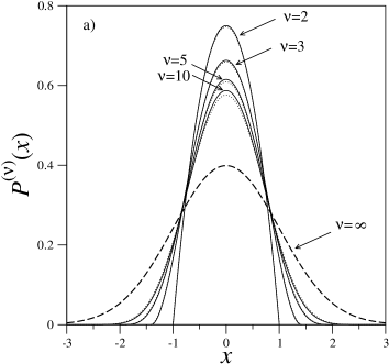
Figure 1: a) Dotted lines: Probability distributions ${\mathcal{P}^{(\nu)}(x)}=\frac{N}{2\sqrt{\nu-1}}p^{(\nu)}_{N,n}$, with $p^{(\nu)}_{N,n}$ given in (9) for $N=500$ and $\nu=2,3,5$ and 10. Solid lines: Corresponding $q_{\text{lim}}$-Gaussians with $q_{\text{lim}}$ given in (17) for the respective values $q_{\text{lim}}=0,1/2,3/4$ and $8/9$. The limiting case $\nu\to\infty$ (Gaussian) is also depicted for comparison. b) ${\mathcal{P}^{(5)}(x)}$ for $N=100,200,500$ and $1000$ and the corresponding $q_{\text{lim}}-$Gaussian with $q_{\text{lim}}=3/4$.

Figure 2 shows that, in what concerns extensivity, the family of triangles (5) follows the Boltzmann-Gibbs prescription, that is, the value of $q$ that makes the $q-$entropy extensive is $q_{\text{ent}}=1$ for all values of $\nu$.

As a last remark, let us associate with the $N$ random variables the variables $\sigma_{i}\equiv 2x_{i}-1=\pm 1$ ($i=1,2,...,N$), so that $\langle\sigma_{i}\rangle=0,\,\forall i$. We can straightforwardly prove that $\langle\sigma_{i}\sigma_{j}\rangle=\frac{1}{2\nu+1}$, $\forall i\neq j$, $\forall N$. In the limit $\nu\to\infty$ we recover $\langle\sigma_{i}\sigma_{j}\rangle=0$, as expected for independent variables, where no correlation exists.

Figure 2: The $q-$entropy $S_{q}=\frac{1-\sum_{n=0}^{N}\binom{N}{n}\left(r_{N,n}^{(\nu)}\right)^{q}}{q-1}$as a function of $N$ for $\nu=1$ (left), $\nu=2$ (center), and $\nu=5$ (right), and typical values of $q$. In all cases $q_{\text{ent}}=1$.

IV SECOND MODEL: DISCRETIZED $q$–GAUSSIANS

We will now introduce another probabilistic model in which we impose a priori the condition that the $N\to\infty$ limit for the probability distribution is a $q-$Gaussian, with the aim to study whether (strict or asymptotic) scale invariance is also obtained. In order to verify if the concept of $q$-independence, i.e. correlations leading to $q$-Gaussians, can be related to scale invariance in probabilistic terms, relation (3) is expected to be satisfied at least in the limit $N\to\infty$, i.e., asymptotically.

Considering again the set of $N$ equally probable binary variables, the correlations will now be given in the form

$$r_{N,n}=\frac{p_{q}(x_{N,n})}{\displaystyle\binom{N}{n}\sum_{n=0}^{N}p_{q}(x_{N,n})}$$ (19)

where $x_{N,n}$ are $N+1$ equally spaced points in the support of the $q$–Gaussian $p_{q}(x)$, to be specified later. For the set of probabilities we again write $p_{N,n}=\binom{N}{n}r_{N,n}$, which provides us with a discrete probability distribution which, by construction, follows the shape of the $q$–Gaussian $p_{q}(x)$.

Concerning the way to choose the points $x_{N,n}$ in (19) a distinction must be made between cases $q<1$ and $q\geqslant 1$.

As mentioned before, for $q<1$, $q$–Gaussians have compact and symmetric support of width $\Delta\equiv 2/\sqrt{(1-q)}$. For this case, we will consider two different ways to choose the points $x_{N,n}$ in the support of the $q$–Gaussian:

1) $N+2$ discretization (D1):

In this implementation, we take $x_{N,n}=x_{\text{min}}+(n+1)h$, for $n=0,1,\dots,N$, with $x_{\text{min}}=-\Delta/2$ and $h=\Delta/(N+2)$, i.e., explicitly, $x_{N,n}=x_{\text{min}}+h,x_{\text{min}}+2h,x_{\text{min}}+3h,...,x_{\text{min}}+(N+1)h$.

2) $N+1$ discretization (D2):

Now, the points $x_{N,n}$ are chosen differently: the same initial interval $\Delta$ breaks now into $N+1$ equal subintervals (not $N+2$ as before) of width $h=\Delta/(N+1)$ and we take the values of $p_{q}(x_{N,n})$ in the center of each subinterval, i.e. $x_{N,n}=x_{\text{min}}+(2n+1)h/2$. The whole set reads $x_{N,n}=x_{\text{min}}+h/2,x_{\text{min}}+3h/2,x_{\text{min}}+5h/2,...,x_{\text{min}}+(2N+1)h/2$.

In contrast, for $q\geqslant 1$, the support for $q$–Gaussians is the whole real axis and we must take this into account in the fit. We will take an increasing width for the fit interval in the form $\Delta_{N}=\delta(N+1)^{\gamma}$, $\delta$ being some initial width, and $\gamma$, with $0\leqslant\gamma\leqslant 1$, a parameter determining the growth of the interval width (for $\gamma=0$ we recover the $q<1$ case). Now $x_{N,n}=x_{\text{min},N}+(n+1)h_{N}$, with $x_{\text{min},N}=-\Delta_{N}/2$ and $h_{N}=\Delta_{N}/(N+2)$.

Despite the fact that different discretizations yield different triangles (19) for a given value of $q$, let us emphasize that the corresponding limiting distributions $p_{N,n}$ tend to the same $q-$Gaussian $p_{q}(x)$ in the limit $N\to\infty$.

Now the following question arises. Do the triangles (19) satisfy relation (3) as the triangles (5) from Sec. III do? In other words, can $q$–Gaussians be related to strictly scale-invariant distributions? Strictly speaking, they are not, since relation (3) is not exactly fulfilled (except for the case $q=0$ with the first discretization D1, as we will show later), but we will show (analytically in some cases, numerically in others) that these triangles are asymptotically scale-invariant, that is, relation (3) is satisfied for $N\to\infty$, or, alternatively, the ratio

$$Q_{N,n}\equiv\frac{r_{N,n}}{r_{N+1,n}+r_{N+1,n+1}}$$ (20)

tends to 1 (or equivalently $Q_{N,n}-1$ tends to 0) as $N$ increases. Note that $Q_{0,0}=Q_{1,0}=Q_{1,1}=1$ for arbitrary values of $r_{0,0}$, $r_{1,n}$ and $r_{2,n}$.

IV.1 The $q<1$ case

Figure 3 shows $Q_{N,n}-1$ as a function of $n$ for $N=500$ and different values of $q$, for both the D1 and D2–discretizations. It is clearly observed the proximity of $Q_{N,n}$ to 1, which is more noticeable in the center of the triangle.

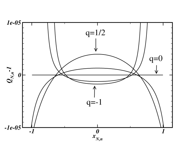
Figure 3: $Q_{N,n}-1$ as a function of $x_{N,n}$ for $N=500$ and different values of $q=-1,-1/2,0,1/4,1/2$ for discretizations D1 (top) and D2 (bottom). Strict scale invariance is observed for $q=0$ and discretization D1. In the rest of the cases deviation from zero is small and, as can be seen by results not shown here, decreases when increasing $N$.

Quite remarkably, for $q=0$, strict scale invariance is obtained in the first discretization, that is, $Q_{N,n}=1$ for all $N$ and $n$. This is so because, in this case, it can be proved that triangle (19) exactly coincides with the Leibnitz-like triangle of the family (5) with $\nu=2$, with associated probabilities $p^{(2)}_{N,n}=\binom{N}{n}r^{(2)}_{N,n}=6[1+n(N-n)/(N+1)]/(N+2)(N+3)$.

An exact expression for $r_{N,n}$ and hence $Q_{N,n}$ can also be obtained for the D2 discretization and $q=0$, the probabilities being in this case $p_{N,n}=3[(2n+1)(2N-2n+1)]/[(N+1)(2N^{2}+4N+3)]$. Of particular interest are the central value, $Q_{c}\equiv Q_{N,N/2}$, and the boundary one, $Q_{0}\equiv Q_{N,0}$, of quotient (20), being given by

$$Q_{c} = \frac{(N+2)^{2}N(2N^{2}+8N+9)}{(2N^{2}+4N+3)(N^{3}+6N^{2}+10N+2)}~{}~{}~{}\qquad\text{for odd $N$,}$$ (21)

$$Q_{0} = \frac{(2N+1)(N+2)(2N^{2}+8N+9)}{(2N^{2}+4N+3)(2N^{2}+11N+6)}~{}.$$ (22)

From Eqs. (21) and (22) results $Q_{c}-1\sim N^{-2}$ and $Q_{0}-1\sim-N^{-1}$, respectively. Though this equations are only valid for $q=0$, this trend is observed for any value of $q<1$. Figure 4 shows in a log-log plot $Q_{c}-1$ as a function of $N$ for different values of $q<1$ and both discretizations. It is clear that the decay follows a $1/N^{2}$ power-law for large $N$ and any value of $q$. No substantial differences are observed between both discretizations.

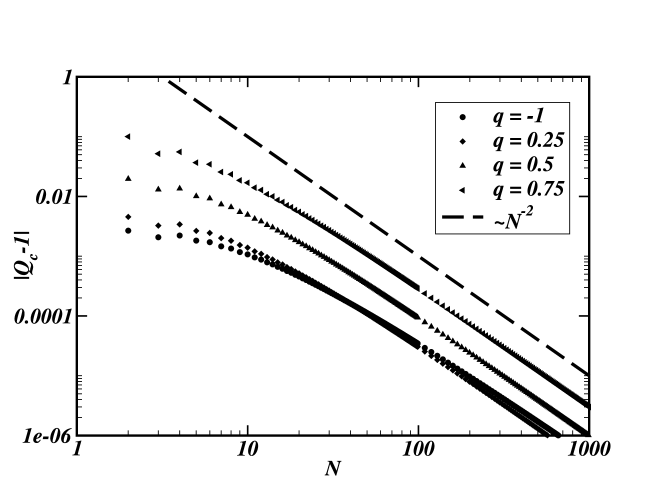
Figure 4: Central ratio $Q_{c}-1$ as a function of $N$ for discretized $q-$Gaussians with $q=-1,0,1/4,1/2$ and $3/4$ for discretizations D1 (top) and D2 (bottom). Exact result (21) for $q=0$ is also shown for D2 discretization. The power law with exponent $-2$ is shown for comparison.

Analogously, Fig. 5 shows $Q_{0}-1$ as a function of $N$ and different values of $q$. We observe now a $1/N$ power-law. We found that this $1/N$ power-law transforms into the $1/N^{2}$ when we do not take into account the complete interval of the compact support of the $q$–Gaussian under consideration (not shown).

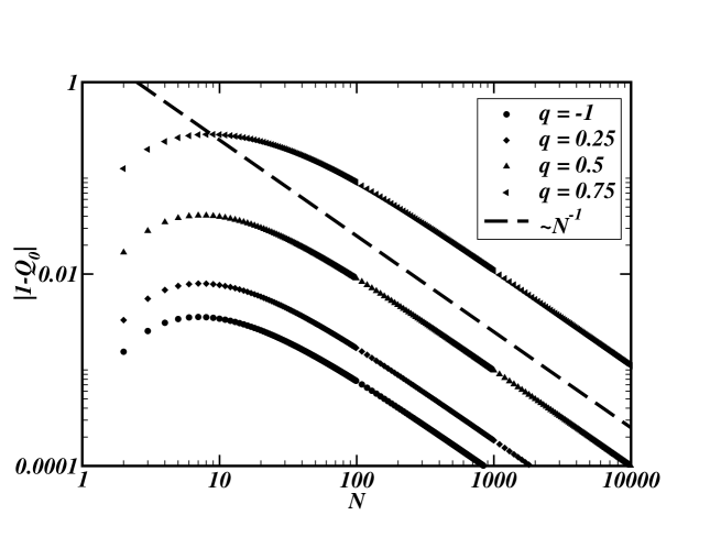
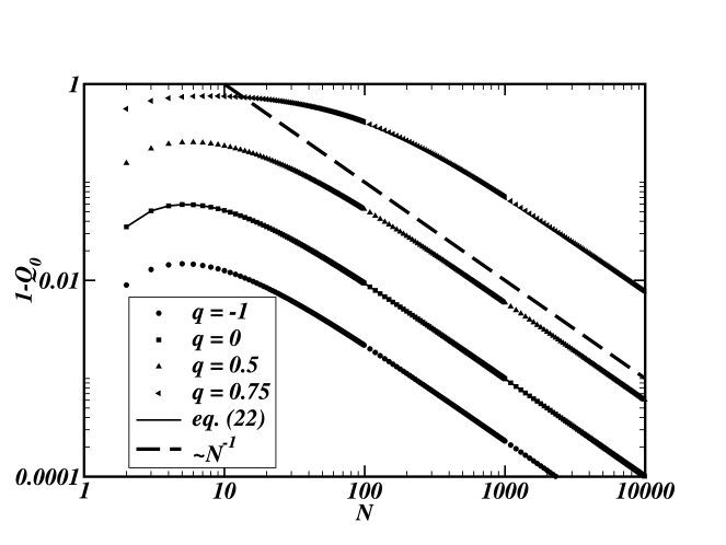
Figure 5: Boundary ratio $Q_{0}-1$ as a function of $N$ for discretized $q-$Gaussians with $q=-1,0,1/4,1/2$ and $3/4$ for discretizations D1 (top) and D2 (bottom). Exact result (22) for $q=0$ is also shown for D2 discretization. The power law with exponent $-1$ is shown for comparison.

Concerning the extensivity of $S_{q}$, the same behavior as in the previous systems is found. We get $q_{\text{ent}}=1$ no matter the value of $q\leqslant 1$ of the discretized $q$–Gaussian (let us remind that there is no reason for the value of $q$ of the discretized $q-$Gaussian be equal, or even simply related, to the index $q_{\text{ent}}$ corresponding to the extensivity of the entropy $S_{q}(N)$), and no matter the type of discretization (D1 or D2). Figure 6 shows the $q-$entropy for discretized $q$–Gaussians for typical values of $q$. The results are independent of the discretization.

Figure 6: $q-$entropy $S_{q}=\frac{1-\sum_{n=0}^{N}\binom{N}{n}r_{N,n}^{q}}{q-1}$, with $r_{N,n}$ given in (19), as a function of $N$ for discretized $q$–Gaussians with $q=-1$ (left), $q=-1/2$ (center), and $q=1/2$ (right) and discretization D1. Results with discretization D2 are indistinguishable. In all cases $q_{\text{ent}}=1$.

IV.2 The $q\geqslant 1$ case

A similar trend is observed for $q\geqslant 1$. Quotients $Q_{0}$ and $Q_{c}$ tend to 1 as $N$ increases for all values of $\gamma$, which, as mentioned before, determines the growth of the interval where the $q-$Gaussian is evaluated. In the case of the Gaussian, i.e. $q=1$, it is known that $\gamma=1/2$. Figure 7 shows the decay of the central quotient for $q=3/2$ and different values of $\gamma$. Apparently, $\gamma=1/2$ provides the appropriate growth of the interval for $q$–Gaussians with $q>1$ as well. For $\gamma<1/2$, one observes the power-law behavior only over some range whereas for $\gamma>1/2$ the decay follows a power-law with an exponent larger than $-1$. The boundary ratio displays the same dependence on $\gamma$.

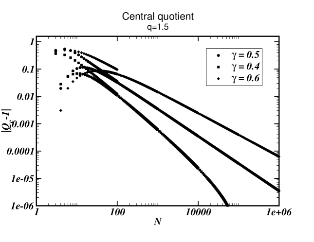
Figure 7: Central ratio $|Q_{c}-1|$ as a function of $N$ for $q=3/2$, $\delta=2$ and $\gamma=$0.4, 0.5 and 0.6. Asymptotic power law behavior with exponent dependent on $\gamma$ is observed for $\gamma\geqslant 1/2$. For $\gamma=1/2$ $Q_{c}-1\sim N^{-1}$, the decay being slower for greater $\gamma$.

For $\gamma=1/2$ we verify a $1/N$ power-law. Figure 8 shows $Q_{c}-1$ and $Q_{0}-1$ for typical values of $q$ and $\gamma=1/2$.

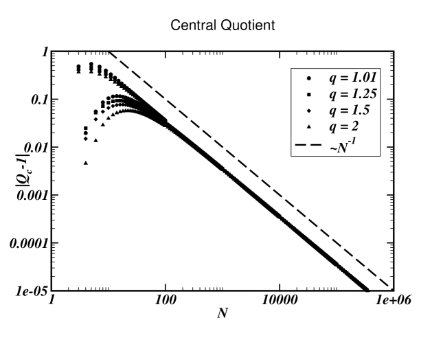
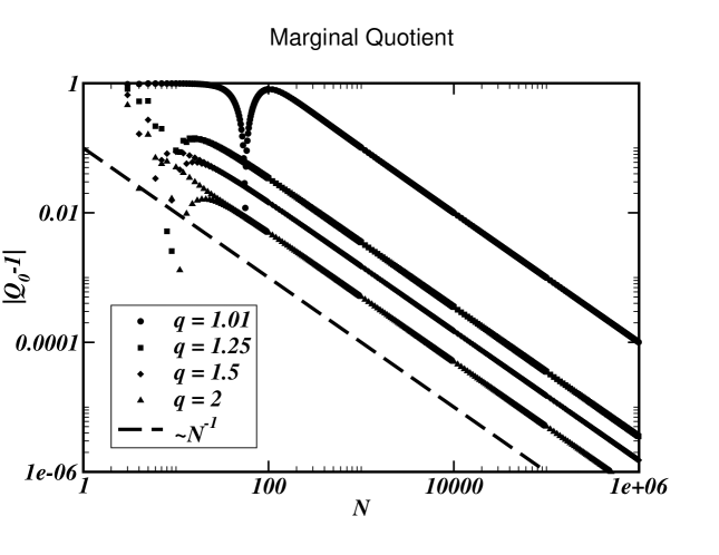
Figure 8: Central quotient (top) and boundary quotient (bottom) decay as a function of $N$ for discretized $q-$Gaussians with $q=1.01$, 1.25, 1.25 and 2, $\gamma=1/2$ and $\delta=2$. In all cases the trend $Q_{0}-1\sim Q_{c}-1\sim N^{-1}$ is observed.

In what concerns the extensivity of the entropy $S_{q}$, the value of $q_{\text{ent}}$ remains 1 and is independent of $\gamma$. Figure 9 shows the $S_{q}(N)$ for typical values of $q\geqslant 1$.

Figure 9: $q-$entropy as in FIG. 6 for discretized $q-$Gaussians with $q=1$ (left), $q=3/2$ (center), and $q=2$ (right). In all cases $q_{\text{ent}}=1$.

V THIRD MODEL: ANOTHER FAMILY OF GENERALIZED TRIANGLES

As seen in Sections III and IV, strictly as well as asymptotically scale-invariant probability models may lead to $q-$Gaussian limiting distributions. Nevertheless, as we already now Hilhorst:07 , scale-invariance does not guarantee $q-$Gaussianity. In this Section, we present a last model to emphasize this point.

The following strictly scale-invariant triangle

$(N=0)\quad\quad$

1

$(N=1)\quad\quad$

$\dfrac{1}{2}$

$\dfrac{1}{2}$

$(N=2)\quad\quad$

$\dfrac{4}{14}$

$\dfrac{3}{14}$

$\dfrac{4}{14}$

$(N=3)\quad\quad$

$\dfrac{5}{28}$

$\dfrac{3}{28}$

$\dfrac{3}{28}$

$\dfrac{5}{28}$

$(N=4)\quad\quad$

$\dfrac{7}{56}$

$\dfrac{3}{56}$

$\dfrac{3}{56}$

$\dfrac{3}{56}$

$\dfrac{7}{56}$

$(N=5)\quad\quad$

$\dfrac{11}{112}$

$\dfrac{3}{112}$

$\dfrac{3}{112}$

$\dfrac{3}{112}$

$\dfrac{3}{112}$

$\dfrac{11}{112}$

$\vdots$

$\vdots$

$\vdots$

with coefficients ($\chi=3/7$) given by

$$r_{N,n}=\left\{\begin{array}[]{lcl}\dfrac{1}{2}-\chi(1-2^{1-N});&&n=0,N\\ \vspace*{-.2cm}\\ \chi 2^{1-N};&&n\neq 0,N\end{array}\right.$$ (23)

corresponds to a different way to introduce correlations in the system. In order to get nonnegative coefficients, the parameter $\chi$ is kept within $[0,1/2]$.

The probabilities are given by

$$p_{N,n}=\left(\dfrac{1}{2}-\chi\right)(\delta_{n,0}+\delta_{n,N})+\binom{N}{n}\chi 2^{1-N}~{}.$$ (24)

The case of binary random variables ($\nu\to\infty$ of the triangles analyzed in Sec. III) is reproduced here for $\chi=1/2$, hence $p_{N,n}=\binom{N}{n}2^{-N}~{}$.

In order to calculate the limiting probability function, the CLT states that the new variable $x=(n-N/2)/(\sqrt{N}/2)$ provides a normal distribution in the limit $N\to\infty$ for the second term of Eq. (24). In addition, two delta peaks appear after substitutions $\delta_{n,0}\to\delta(\frac{\sqrt{N}}{2}x+\frac{N}{2})=\frac{2}{\sqrt{N}}\delta(x+\sqrt{N})$ and $\delta_{n-N,0}\to\delta(\frac{\sqrt{N}}{2}x-\frac{N}{2})=\frac{2}{\sqrt{N}}\delta(x-\sqrt{N})$. Finally, by taking limits in Eq. (24), we obtain

$$\mathcal{P}(x)=\lim\limits_{N\to\infty}\frac{\sqrt{N}}{2}p_{N,n}=2\chi\frac{1}{\sqrt{2\pi}}e^{-x^{2}/2}+\left(\frac{1}{2}-\chi\right)\lim_{N\to\infty}(\delta(x-\sqrt{N})+\delta(x+\sqrt{N}))$$ (25)

which consists of a Gaussian distribution plus the additional contribution of the delta peaks corresponding to a concentration of probability on the two sides of the triangle.

As in the previous sections, the BG–entropy is extensive for this triangle as well. This may be proved directly by inserting coefficients (24) into

$$S_{1}=-\sum\limits^{N}_{n=0}\binom{N}{n}r_{N,n}\ln{r_{N,n}}$$ (26)

yielding

$$S_{1} =-(1-\chi)\ln[(\dfrac{1}{2}-\chi)+\chi 2^{1-N}]-\chi 2^{1-N}\sum\limits^{N-1}_{n=1}\binom{N}{n}[\ln(\chi 2^{1-N})]$$

$$=(\chi-1)\ln[(\dfrac{1}{2}-\chi)+\chi 2^{1-N}]-2\chi\left(\ln(2\chi)-2^{1-N}\ln(\chi 2^{1-N})\right)+2\chi N\ln 2$$

$$\propto N$$ (27)

for large $N$.

VI CONCLUSIONS

A family of Leibnitz-like triangles, leading to $q$–Gaussians as limiting probability distribution functions with $q\leqslant 1$, was introduced, where the limiting distribution could be exactly calculated. These systems correspond to $N$ correlated binary random variables, the index $q$ characterizing the strength of correlation. The case $q\to-\infty$ corresponds to very strongly correlated variables giving a uniform limiting distribution.

On the other hand, the coefficients of another type of triangles were constructed by discretizing $q$–Gaussians. These triangles, having now by construction $q$–Gaussians with $q<1$ as limiting probability functions, showed a behavior with depends on the specific discretization of the support interval. Except for one particular case, the Leibnitz rule, related to system size scale invariance of the probabilities, is only asymptotically satisfied. The system approaches scale invariance with a $1/N^{2}$ power-law for large $N$, except for the boundary coefficients where the convergence to scale invariance is much slower, of the type $1/N$. The $1/N^{2}$ law makes a crossover into a $1/N$ one over the entire triangle when considering $q$–Gaussians with $q\geqslant 1$.

Finally, another family of strictly scale-invariant triangles with a rather strange limiting distribution function was introduced. In the limit $N\to\infty$, the triangles yield a Gaussian distribution together with two delta peaks centered at points going to infinity.

The BG–entropy remains extensive for all three types of triangles, equally to previously studied Leibnitz–like triangles MoyanoGellmann:2006 . This may be the result of the simplicity of the models presented in this paper. More sophisticated models, as for instance the Hamiltonian mean field model (see for instance ref. Pluchino:07 ; Pluchino:08 ), appear to approach a $q$–Gaussian characterized by a non-equilibrium stationary state with the $q$–entropy possibly being extensive for $q\neq 1$. However, in the present effort we are here not particularly interested in the general relation between the extensivity of the entropy and stationary-state probability distributions, but we rather searched to find out which kind of correlation between the microscopic events of a system leads to $q$–Gaussians as limiting distributions (possibly, as attractors).

The Leibnitz rule provides a simple tool to study models composed of correlated binary random variables, and enabled the exact calculation of their limiting functions. As already addressed in  Hilhorst:07 , this rule cannot be uniquely related to nonextensive thermostatistics. Indeed, Leibnitz-like triangles exist which precisely lead to $q$–Gaussians (as shown in the present paper) as well as to other limiting probability functions (as shown in Hilhorst:07 , and also here). Additionally, the present second family of triangles (with asymptotic but not strict scale invariance) also tended to a $q$–Gaussian. The scenario which emerges is that asymptotic validity of the Leibnitz rule might represent a necessary but surely not sufficient condition for the system to tend to $q$–Gaussians as limiting distributions when $N\to\infty$.

The fact that different implementations of correlations between the variables of a system can lead to the same function, — $q$–Gaussians in the present case —, can be seen as a hint for these functions being attractors for a variety of different systems, and so supports the demand of generality of the $q$-generalized central limit theorem presented in  Tsallis:05 ; Umarov:08 ; Umarov:06a ; Umarov:07 . However, to assure the applicability of this central limit theorem, the stability of the $q$–Gaussians as limiting functions of the systems presented here needs to be proved, either by establishing that the correlations correspond to $q$-independence, or by introducing, for example, weak perturbations.

- (1) C. Tsallis, M. Gell-Mann, and Y. Sato, Proc. Natl. Acad. Sc. (USA) 102, 15377 (2005).
- (2) S. Umarov, C. Tsallis and S. Steinberg, Milan J. Math. 76, DOI 10.1007/s00032-008-0087-y (2008).
- (3) S. Umarov, C. Tsallis, M. Gell-Mann and S. Steinberg, condmat/0606038 and condmat/0606040 (2006).
- (4) S. Umarov and C. Tsallis, condmat/0703533 (2007).
- (5) S. Umarov and C. Tsallis, in Complexity, Metastability and Nonextensivity, eds. S. Abe, H.J. Herrmann, P. Quarati, A. Rapisarda and C. Tsallis, American Institute of Physics Conference Proceedings 965, 34 (New York, 2007).
- (6) S. Umarov and C. Tsallis, Phys. Lett. A 372, 4874 (2008).
- (7) S. Umarov and S.M.D. Queiros, 0802.0264 [cond-mat.stat-mech] (2008).
- (8) C. Tsallis and S.M.D. Queiros, in Complexity, Metastability and Nonextensivity, eds. S. Abe, H.J. Herrmann, P. Quarati, A. Rapisarda and C. Tsallis, American Institute of Physics Conference Proceedings 965, 8 (New York, 2007).
- (9) S.M.D. Queiros and C. Tsallis, in Complexity, Metastability and Nonextensivity, eds. S. Abe, H.J. Herrmann, P. Quarati, A. Rapisarda and C. Tsallis, American Institute of Physics Conference Proceedings 965, 21 (New York, 2007).
- (10) C. Vignat and A. Plastino, J. Phys. A 40, F969 (2007).
- (11) L.G. Moyano, C. Tsallis, and M. Gell-Mann, Europhys. Lett. 73, 813 (2006).
- (12) W. Thistleton, J.A. Marsh, K. Nelson, and C. Tsallis, unpublished.
- (13) H.J. Hilhorst and G. Schehr, J. Stat. Mech., P06003 (2007).
- (14) C. Tsallis, J. Stat. Phys. 52 479, (1988).
- (15) M. Gell-Mann and C. Tsallis, editors, Nonextensive Entropy - Interdisciplinary Applications (Oxford University Press, New York, 2004).
- (16) J. P. Boon and C. Tsallis, editors. Nonextensive Statistical Mechanics: New Trends, New Perspectives, Europhysics News 36 (6) (2005) [Errata: 37 25 (2006)]; C. Tsallis, Entropy, in Encyclopedia of Complexity and Systems Science (Springer, Berlin, 2008), in press.
- (17) For a regularly updated bibliography, see http://tsallis.cat.cbpf.br/biblio.htm
- (18) P. Douglas, S. Bergamini and F. Renzoni, Phys. Rev. Lett. 96, 110601 (2006).
- (19) B. Liu and J. Goree, Phys. Rev. Lett. 100, 055003 (2008).
- (20) A. Upaddhyaya, J.P. Rieu, J.A. Glazier, and Y. Sawada, Physica A 293, 459 (2001).
- (21) K.E. Daniels, C. Beck, and E. Bodenschatz, Physica D 193, 208 (2004).
- (22) L. Nivanen, A. Le Mehaute and Q.A. Wang, Rep. Math. Phys. 52, 437 (2003).
- (23) E.P. Borges, Physica A 340 95 (2004).
- (24) C. Beck and and F. Schlogl, Thermodynamics of Chaotic Systems (Cambridge University Press, Cambridge, 1993).
- (25) C. Tsallis, A.R. Plastino and R.F. Alvarez-Estrada, 0802.1698 [cond-mat.stat-mech] (2008).
- (26) A. Pluchino, A. Rapisarda and C. Tsallis, Europhys. Lett. 80 26002 (2007).
- (27) A. Pluchino, A. Rapisarda and C. Tsallis, Physica A 387, 3121 (2008).
- (28) U. Tirnakli, C. Beck and C. Tsallis, Phys. Rev. E 75, 040106(R) (2007).
- (29) U. Tirnakli, C. Tsallis and C. Beck, 0802.1138 [cond-mat.stat-mech] (2008).
- (30) C. Tsallis and D. J. Bukman, Phys. Rev. E 54, R2197 (1996).
- (31) D. Prato and C. Tsallis, Phys. Rev. E 60, 2398 (1999).
- (32) G.A. Tsekouras, A. Provata and C. Tsallis, Phys. Rev. E 69, 016120 (2004).
- (33) C. Anteneodo, Eur. Phys. J. B 42, 271 (2004).