Holomorphic Representation of Constant Mean Curvature Surfaces in Minkowski Space: Consequences of Non-Compactness in Loop Group Methods

Abstract.

We give an infinite dimensional generalized Weierstrass representation for spacelike constant mean curvature (CMC) surfaces in Minkowski 3-space ${\mathbb{R}}^{2,1}$. The formulation is analogous to that given by Dorfmeister, Pedit and Wu for CMC surfaces in Euclidean space, replacing the group $SU_{2}$ with $SU_{1,1}$. The non-compactness of the latter group, however, means that the Iwasawa decomposition of the loop group, used to construct the surfaces, is not global. We prove that it is defined on an open dense subset, after doubling the size of the real form $SU_{1,1}$, and prove several results concerning the behavior of the surface as the boundary of this open set is encountered. We then use the generalized Weierstrass representation to create and classify new examples of spacelike CMC surfaces in ${\mathbb{R}}^{2,1}$. In particular, we classify surfaces of revolution and surfaces with screw motion symmetry, as well as studying another class of surfaces for which the metric is rotationally invariant.

Introduction

0.1. Motivation

It is well known that minimal surfaces in Euclidean $3$-space have a Weierstrass representation in terms of holomorphic functions, and that the Gauss map of such a surface is holomorphic. For non-minimal constant mean curvature (CMC) surfaces, Kenmotsu [21] showed that the Gauss map is harmonic, and gave a formula for obtaining CMC surfaces from any such harmonic maps. On the other hand, as a result of work by Pohlmeyer [26], Uhlenbeck [35] and others, it became known that harmonic maps from a Riemann surface into a symmetric space $G/H$ can be lifted to holomorphic maps into the based loop group $\Omega G$, satisfying a horizontality condition - see [16] for the history. Subsequently, Dorfmeister, Pedit and Wu [14] gave a method, the so-called DPW method, for obtaining such harmonic maps directly from a certain holomorphic map into the complexified loop group $\Lambda G^{\mathbb{C}}$, via the Iwasawa splitting of this group, $\Lambda G^{\mathbb{C}}=\Omega G\cdot\Lambda^{+}G^{\mathbb{C}}$. This method has the advantage that the holomorphic loop group map itself is obtained from a collection of arbitrary complex-valued holomorphic functions. Combined with the Sym-Bobenko formula, discussed below, for obtaining a surface from its loop group extended frame, this gives an infinite dimensional “generalized Weierstrass representation” for CMC surfaces in terms of holomorphic functions.

Integrable systems methods have been shown to have many applications in submanifold theory. Concerning CMC surfaces, notable early results were the classification of CMC tori in $\mathbb{R}^{3}$ by Pinkall and Sterling [25], and the rendering of all CMC tori in space forms in terms of theta functions by Bobenko [5]. The DPW method has led to new examples of non-simply-connected CMC surfaces in $\mathbb{R}^{3}$ - and other space forms - that have not yet been proven to exist by any other approach [22], [23], [29].

Unsurprisingly, an analogous construction is obtained for spacelike, which is to say Riemannian, CMC surfaces in Minkowski space $\mathbb{R}^{2,1}$, by replacing the group $SU_{2}$, used in the Euclidean case, with the non-compact real form $SU_{1,1}$. However, there is a major difference, in that the Iwasawa decomposition is not global when the underlying group is non-compact, which has consequences for the global properties of the surfaces constructed.

There is already an extensive collection of work about spacelike non-maximal CMC surfaces in $\mathbb{R}^{2,1}$ and their harmonic ([24]) Gauss maps. Works of Treibergs [34], Wan [36], and Wan-Au [37] show existence of a large class of entire examples, which are then necessarily complete (Cheng and Yau [10]). Other studies, also without the loop group point of view, include [11] and [1]. Inoguchi [18] gave a loop group formulation and discussed finite type solutions and solutions obtained via dressing, which are two further methods, distinct from the DPW method employed here, that can also be used for loop group type problems.

Studying the generalized Weierstrass representation for CMC surfaces in ${\mathbb{R}}^{2,1}$ is interesting for various reasons: from the viewpoint of surface theory, there is naturally a richer variety of such surfaces, compared to the Euclidean case, due to the fact that not all directions are the same in Minkowski space. CMC surfaces in Minkowski space are important in the study of classical relativity - see for example, the work of Bartnik and Simon [4, 3]. The main issue addressed in those works was to give conditions which would guarantee that surfaces obtained from a variational problem are everywhere spacelike. The holomorphic representation studied here is a completely different approach: all surfaces are, in principle, obtained from this method and the surface is guaranteed to be spacelike as long as the holomorphic loop group map takes its values in an open dense subset of the loop group (the “big cell”). The surface fails to be spacelike or immersed only when the corresponding holomorphic data encounters the boundary of this dense set. Since all CMC surfaces have such a representation, understanding the behavior at this boundary potentially gives a means to characterize the singularities. More generally in the context of integrable systems in geometry, this example can be thought of as a test case regarding the significance of the absence of a global Iwasawa decomposition, or, more broadly, of the non-compactness of the group.

0.2. Results

In Sections 1 and 2 we present the Iwasawa decomposition associated to the group of loops in $SU_{1,1}$. The general case for non-compact groups had been earlier treated by Kellersch [20]; we provide a rather explicit proof for our case. The main new result here, which is important for our applications, is that, after doubling the size of the group, by setting $G=SU_{1,1}\,\sqcup\,i\sigma_{1}\cdot SU_{1,1}$, where $\sigma_{1}$ is a Pauli matrix, we are able to prove that the Iwasawa splitting we need is almost global. That is, if $\Lambda G^{\mathbb{C}}$ is the group of loops in a complexification $G^{\mathbb{C}}$ of $G$, $\Lambda^{+}G^{\mathbb{C}}$ is the subgroup of loops which extend holomorphically to the unit disc, and $\Omega G$ is the subgroup of based loops mapping 1 to the identity, then

(1) $$\Omega G\cdot\Lambda^{+}G^{\mathbb{C}}$$

is an open dense subset, called the (Iwasawa) big cell, of $\Lambda G^{\mathbb{C}}$. We are primarily interested in this result in the twisted setting, described in Section 2.

We also prove, in Section 1.4, that, for a loop which extends meromorphically to the unit disk with exactly one pole, the Iwasawa decomposition can be computed explicitly using finite linear algebra. This result is used for the analysis of singularities arising in CMC surfaces.

In Section 3 we give the loop group formulation and the DPW method for CMC surfaces in Minkowski space. This uses the first factor $F$ of the decomposition $\phi=FB$, corresponding to (1), to obtain a CMC surface from a certain holomorphic map $\phi:\Sigma\to\Lambda G^{\mathbb{C}}$, where $\Sigma$ is a Riemann surface.

In Section 4 we examine the behavior of the surfaces at the boundary of the big cell. In Theorem 4.1, we prove that the DPW construction maps an open dense set $\Sigma^{\circ}\subset\Sigma$ to a smooth CMC surface, and that the singular set, $\Sigma\setminus\Sigma^{\circ}$ is locally given as the zero set of a non-constant real analytic function.

The boundary of the big cell is a countable disjoint union of “small cells”, the first two of which are of lowest codimension in the loop group, and therefore the most significant. We examine the behavior of the surface as points on the set $\Sigma\setminus\Sigma^{\circ}$ which correspond to the first two small cells are approached. In Theorem 4.2, we prove that the surface always has finite singularities at points which are mapped by $\phi$ to the first small cell (and this also occurs along the zero set of a non-constant real analytic function). On the other hand, we prove that, as points mapping to the second small cell are approached, the surface is always unbounded and the metric blows up.

The next two sections are devoted to applications. There are a variety of CMC rotational surfaces in ${\mathbb{R}}^{2,1}$, because the rotation axes can be either timelike or spacelike or lightlike. Classifications of such rotational surfaces were considered by Hano and Nomizu [17] and Ishihara and Hara [19], with the aim of studying rolling curve constructions for the profile curves, but the moduli space was not considered. Here we find the moduli spaces for both surfaces of revolution and the more general class of equivariant surfaces. In Section 5, we explicitly construct and classify all spacelike CMC surfaces of revolution in $\mathbb{R}^{2,1}$. In particular, this results in a new family of loops for which we know the explicit $SU_{1,1}$-Iwasawa splitting. We also study the surfaces in the associate families of the CMC surfaces of revolution, which we prove give all spacelike CMC surfaces with screw motion symmetry (equivariant surfaces). In both those cases, the explicit nature of the construction can be used to study the singularities and the end behaviors of the surfaces.

In Section 6 we use the Weierstrass representation to construct $\mathbb{R}^{2,1}$ analogues of Smyth surfaces [31] (surfaces whose metrics have a rotational symmetry), and study their properties.

1. The Iwasawa decomposition for the untwisted loop group

If $G$ is a compact semisimple Lie group, then the Iwasawa decomposition of $\Lambda G$, proved in [27], is

(2) $$\Lambda G^{\mathbb{C}}=\Omega G\cdot\Lambda^{+}G,$$

where $\Omega G$ is the set of based loops $\gamma\in\Lambda G$ such that $\gamma(1)=1$. For non-compact groups, this problem was investigated by Kellersch [20]. An English presentation of those results can be found in the appendix of [2]. Here we restrict to $SU_{1,1}$, as it is a representative example, and as it has applications to CMC surface theory.

1.1. Notation and definitions

Throughout this article we will make extensive use of the Pauli matrices

$$\sigma_{1}:=\begin{pmatrix}0&1\\ 1&0\end{pmatrix}\;,\;\;\sigma_{2}:=\begin{pmatrix}0&-i\\ i&0\end{pmatrix}\;,\;\;\sigma_{3}:=\begin{pmatrix}1&0\\ 0&-1\end{pmatrix}\;.$$

Let $\mathbb{S}^{1}$ be the unit circle in the complex $\lambda$-plane, $D_{+}$ the open unit disk, and $D_{-}=\{\lambda\in\mathbb{C}\,|\,|\lambda|>1\}\cup\{\infty\}$ the exterior disk in $\mathbb{C}\mathbb{P}^{1}$.

If $G^{\mathbb{C}}$ is any complex semisimple Lie group then $\Lambda G^{\mathbb{C}}$ denotes the Banach Lie group of maps from $\mathbb{S}^{1}$ into $G^{\mathbb{C}}$ with some $H^{s}$-topology, $s>1/2$. All subgroups are given the induced topology. For any subgroup $\mathcal{H}$ of $\Lambda G^{\mathbb{C}}$ we denote the subgroup of constant loops, which is to say $\mathcal{H}\cap G^{\mathbb{C}}$, by $\mathcal{H}^{0}$.

For us, $G^{\mathbb{C}}$ will be the special linear group $SL_{2}\mathbb{C}$. Now the real form $SU_{1,1}$ is the fixed point subgroup with respect to the involution

(3) $$\tau(x)=\textup{Ad}_{\sigma_{3}}(\overline{x^{t}})^{-1}.$$

For our application, however, it will become clear that it is convenient to set

$$G:=\{x\in SL_{2}\mathbb{C}~{}|~{}\tau(x)=\pm x\}.$$

As a manifold, $G$ is a disjoint union $SU_{1,1}\,\sqcup\,i\sigma_{1}\cdot SU_{1,1}$, and has a complexification $G^{\mathbb{C}}=SL_{2}\mathbb{C}$. It turns out that $G$ works just as well as $SU_{1,1}$ for our application, and this choice will mean that the Iwasawa decomposition is almost global. We remark that an alternative way to achieve this would have been to set $G^{\mathbb{C}}$ to be the group $\{x\in GL(2,\mathbb{C})~{}|~{}\det x=\pm 1\}$, and in this case the appropriate real form $G$ would be just the fixed point subgroup with respect to $\tau$.

Let $\Lambda G$ denote the subgroup of $\Lambda G^{\mathbb{C}}$ consisting of loops with values in the subgroup $G$. We extend $\tau$ to an involution of the loop group by the formula

$$(\tau(x))(\lambda) := \tau(x(\bar{\lambda}^{-1}))$$

$$= \sigma_{3}(\overline{x(\bar{\lambda}^{-1})}^{t})^{-1}\sigma_{3}.$$

Then it is easy to verify that the definition of $\Lambda G\subset\Lambda G^{\mathbb{C}}$ is the analogue of $G\subset G^{\mathbb{C}}$:

$$\Lambda G = \{x\in\Lambda G^{\mathbb{C}}~{}|~{}\tau(x)=\pm x\}\;,$$

$$= (\Lambda G^{\mathbb{C}})_{\tau}\,\sqcup\,i\sigma_{1}\cdot(\Lambda G^{\mathbb{C}})_{\tau},$$

where $(\Lambda G^{\mathbb{C}})_{\tau}=\Lambda SU_{1,1}$ is the fixed point subgroup with respect to $\tau$. We want a decomposition similar to the Iwasawa decomposition (2), but our group $G$ is non-compact.

1.1.1. Normalizations for the untwisted setting

Let $\triangle^{+}$ and $\triangle^{-}$ denote the sets of $2\times 2$ upper triangular and lower triangular matrices, respectively, and $\triangle^{\pm}_{\mathbb{R}}$ denote the subsets with the further restriction that the diagonal components are positive and real. For any lie group $X$, let $\Lambda^{\pm}X$ denote the subgroup consisting of loops which extend holomorphically to $D_{\pm}$. We start by defining some further subgroups of the untwisted loop group $\Lambda G^{\mathbb{C}}:=\Lambda SL_{2}\mathbb{C}$. Denote the centers of the interior and exterior disks, $D_{\pm}$, by $\lambda_{+}:=0$ and $\lambda_{-}:=\infty$. Set

$$\Lambda_{\triangle}^{\pm}G^{\mathbb{C}}:=\{B\in\Lambda^{\pm}G^{\mathbb{C}}\,|\,B(\lambda_{\pm})\in\triangle^{\pm}\},$$

$$\Lambda_{{\mathbb{R}}}^{+}G^{\mathbb{C}}:=\{B\in\Lambda^{+}G^{\mathbb{C}}\,|\,B(0)\in\triangle^{+}_{\mathbb{R}}\},$$

$$\Lambda_{I}^{\pm}G^{\mathbb{C}}:=\{B\in\Lambda^{\pm}G^{\mathbb{C}}\,|\,B(\lambda_{\pm})=I\}\;,$$

1.2. The Birkhoff decomposition

To obtain the corresponding results for the twisted loop group later, we normalize the factors in the Birkhoff factorization theorem of [27], in a certain way:

Theorem 1.1.

(Birkhoff decomposition [27]) Any $\phi\in\Lambda G^{\mathbb{C}}$, has a decomposition:

$$\phi=B_{-}MB_{+}\,,\hskip 14.22636ptB_{\pm}\in\Lambda^{\pm}_{\triangle}G^{\mathbb{C}}\,,$$

where either

$$M=\begin{pmatrix}\lambda^{\ell}&0\\ 0&\lambda^{-\ell}\end{pmatrix},\hskip 14.22636pt\textup{or}\hskip 14.22636ptM=\begin{pmatrix}0&\lambda^{\ell}\\ -\lambda^{-\ell}&0\end{pmatrix},\hskip 14.22636pt\ell\in\mathbb{Z}\;.$$

The middle term, $M$, is uniquely determined by $\phi$. The big cell $\mathcal{B}^{U}$, where $l=0$, is open and dense in $\Lambda G^{\mathbb{C}}$, and in this case there is a unique factorization $\phi=\hat{B}_{-}M_{0}\hat{B}_{+}$, with $\hat{B}_{\pm}\in\Lambda_{I}^{\pm}G^{\mathbb{C}}$ and $M_{0}\in G^{\mathbb{C}}$. Moreover, the map $\mathcal{B}^{U}\to\Lambda^{-}_{I}G^{\mathbb{C}}\times G^{\mathbb{C}}\times\Lambda^{+}_{I}G^{\mathbb{C}}$, given by $[\phi\mapsto(\hat{B}_{-},\,M_{0},\,\hat{B}_{+})]$, is a real analytic diffeomorphism.

Proof.

The result is stated and proved in an alternative form as Theorem 8.1.2 and Theorem 8.7.2 of [27], without the upper and lower triangular normalization of the constant terms, and where the middle term, $M$, is a homomorphism from $\mathbb{S}^{1}$ into a maximal torus, which is to say the first type of middle term here. That is

$$\phi=\phi_{-}\begin{pmatrix}\lambda^{l}&0\\ 0&\lambda^{-l}\end{pmatrix}\phi_{+},\hskip 42.67912pt\phi_{\pm}\in\Lambda^{\pm}G^{\mathbb{C}}.$$

Such a product can be manipulated so that the constant terms of $\phi_{\pm}$ are appropriately triangular if one allows the middle term to become off-diagonal. ∎

1.3. The untwisted Iwasawa decomposition for $G$

Define the untwisted Iwasawa big cell

$$\mathcal{B}_{1,1}^{U}:=\{\phi\in\Lambda G^{\mathbb{C}}~{}|~{}(\tau(\phi))^{-1}\phi\in\mathcal{B}^{U}\}.$$

Theorem 1.2.

(Untwisted $SU_{1,1}$ Iwasawa decomposition)

1. The group $\Lambda G^{\mathbb{C}}$ is a disjoint union,

   $$\mathcal{B}_{1,1}^{U}\sqcup\bigsqcup_{m\in\mathbb{Z}}\widehat{\mathcal{P}}_{m},$$

   where $\widehat{\mathcal{P}}_{m}$ are defined below at item (3).

2. Any element $\phi\in\mathcal{B}_{1,1}^{U}$ has a decomposition

   $$\phi=FB,\hskip 42.67912ptF\in\Lambda G,\hskip 14.22636ptB\in\Lambda^{+}_{\triangle}G^{\mathbb{C}}.$$

   We can choose $B\in\Lambda^{+}_{\mathbb{R}}G^{\mathbb{C}}$, and then $F$ and $B$ are uniquely determined, and the product map $\Lambda G\times\Lambda^{+}_{\mathbb{R}}G^{\mathbb{C}}\to\mathcal{B}_{1,1}^{U}$ is a real analytic diffeomorphism. We call this unique decomposition normalized.

3. Any element $\phi\in\widehat{\mathcal{P}}_{m}$ can be expressed as

   $$\phi=F\hat{\omega}_{m}B,\hskip 42.67912ptF\in(\Lambda G^{\mathbb{C}})_{\tau},\hskip 14.22636ptB\in\Lambda^{+}_{\triangle}G^{\mathbb{C}},$$

   where

   $$\hat{\omega}_{m}:=\begin{pmatrix}\frac{1}{2}&\lambda^{m}\\ -\frac{1}{2}\lambda^{-m}&1\end{pmatrix}.$$

4. The Iwasawa big cell $\mathcal{B}^{U}_{1,1}$ is an open dense set of $\Lambda G^{\mathbb{C}}$. The complement of the big cell is locally given as the zero set of a non-constant real analytic function $g:\Lambda G^{\mathbb{C}}\to\mathbb{C}$.

The proof of Theorem 1.2 is a consequence of the following lemma:

Lemma 1.3.

If $\psi\in\Lambda G^{\mathbb{C}}$ satisfies $(\tau(\psi))^{-1}=\psi$, then

$$\psi=(\tau(B_{+}))^{-1}(\pm I)B_{+}\;\;\text{or}\;\;\;\psi=(\tau(B_{+}))^{-1}\begin{pmatrix}0&\lambda^{m}\\ -\lambda^{-m}&0\end{pmatrix}B_{+}$$

for some uniquely determined integer $m$, and for some $B_{+}\in\Lambda_{\triangle}^{+}G^{\mathbb{C}}$.

Proof.

Consider the two cases for the Birkhoff splitting of $\psi$ given in Theorem 1.1. First, if $\psi=B_{-}\text{diag}(\lambda^{k},\lambda^{-k})B_{+}$, then

(5) $$B=B_{+}\tau(B_{-})=\begin{pmatrix}a&b\\ c&d\end{pmatrix}$$

is an element of $\Lambda_{\triangle}^{+}G^{\mathbb{C}}$, and the assumption that $(\tau(\psi))^{-1}=\psi$ is equivalent to the equation

$$\begin{pmatrix}a^{*}\lambda^{-k}&-c^{*}\lambda^{k}\\ -b^{*}\lambda^{-k}&d^{*}\lambda^{k}\end{pmatrix}=\begin{pmatrix}a\lambda^{k}&b\lambda^{k}\\ c\lambda^{-k}&d\lambda^{-k}\end{pmatrix}\;.$$

It follows that $b$ and $c$ are both identically zero, that $a,d$ are constant and real, and that $k=0$. So $B=\text{diag}(\alpha,\alpha^{-1})(\pm I)\text{diag}(\alpha,\alpha^{-1})$ for some constant $\alpha>0$. Then $\psi=(\tau(\psi))^{-1}=(\tau(B_{+}))^{-1}(\tau(B_{-}))^{-1}=\tau(\tilde{B}_{+})^{-1}(\pm I)\tilde{B}_{+}$, where $\tilde{B}_{+}=\text{diag}(\alpha^{-1},\alpha)B_{+}$.

Now consider the case $\psi=B_{-}{\tiny{\begin{pmatrix}0&\lambda^{k}\\ -\lambda^{-k}&0\end{pmatrix}}}B_{+}$. Proceeding as before, we have

$$\begin{pmatrix}a^{*}&-c^{*}\\ -b^{*}&d^{*}\end{pmatrix}\begin{pmatrix}0&\lambda^{k}\\ -\lambda^{-k}&0\end{pmatrix}=\begin{pmatrix}0&\lambda^{k}\\ -\lambda^{-k}&0\end{pmatrix}\begin{pmatrix}a&b\\ c&d\end{pmatrix}\;,$$

where $B$ is as in (5). It follows that $\bar{a}=d$ is constant and $|a|=1$, and $b\cdot c$ is identically zero. Further, when $k<0$, then $b=0$ and $c=c^{*}\lambda^{-2k}$ with a finite expansion in $\lambda$ of the form $c=c_{1}\lambda^{1}+...+c_{-2k-1}\lambda^{-2k-1}$, while, on the other hand, if $k\geq 0$, we have that $c=0$ and $b=b^{*}\lambda^{2k}$, with $b=b_{0}\lambda^{0}+...+b_{2k}\lambda^{2k}$.

Setting $\tilde{B}_{+}=yB_{+}$ and $\tilde{B}_{-}=B_{-}x^{-1}$ then the requirements that $\tilde{B}_{+}\in\Lambda_{\triangle}^{+}G^{\mathbb{C}}$ and that $\psi=(\tau(\tilde{B}_{+}))^{-1}\begin{pmatrix}0&\lambda^{m}\\ -\lambda^{-m}&0\end{pmatrix}\tilde{B}_{+}$ will be satisfied if we can choose $y\in\Lambda^{+}_{\triangle}G^{\mathbb{C}}$ and $x\in\Lambda^{-}_{\triangle}G^{\mathbb{C}}$ with the properties:

$$x^{-1}\begin{pmatrix}0&\lambda^{k}\\ -\lambda^{-k}&0\end{pmatrix}y=\begin{pmatrix}0&\lambda^{k}\\ -\lambda^{-k}&0\end{pmatrix}\;,\hskip 28.45274ptB=y^{-1}\tau(x).$$

Set

$$y=\begin{pmatrix}\sqrt{a}^{-1}&y_{1}\\ y_{2}&\sqrt{a}\end{pmatrix}\;,\hskip 28.45274ptx^{-1}=\begin{pmatrix}\sqrt{a}^{-1}&x_{1}\\ x_{2}&\sqrt{a}\end{pmatrix}\;,$$

then when $k\geq 0$, we can take $(y_{1},y_{2},x_{1},x_{2})=(-\sqrt{a}b/2,0,0,-\sqrt{a}b\lambda^{-2k}/2)$. When $k<0$, we take $(y_{1},y_{2},x_{1},x_{2})=(0,-c/(2\sqrt{a}),-c\lambda^{2k}/(2\sqrt{a}),0)$. ∎

Proof of Theorem 1.2

Proof.

Take any $\phi\in\Lambda G^{\mathbb{C}}$. Set $\psi:=\tau(\phi)^{-1}\phi$. Then $(\tau(\psi))^{-1}=\psi$ and so we can apply Lemma 1.3, which implies that

$$\psi=(\tau(B_{+}))^{-1}\tau(\hat{\omega})^{-1}\hat{\omega}B_{+}\;,$$

where $\hat{\omega}$ is (uniquely) one of the following:

$$\hat{\omega}_{+}=I,\hskip 28.45274pt\hat{\omega}_{-}=\begin{pmatrix}0&1\\ -1&0\end{pmatrix},\hskip 28.45274pt\hat{\omega}_{m}=\begin{pmatrix}\tfrac{1}{2}&\lambda^{m}\\ -\tfrac{1}{2}\lambda^{-m}&1\end{pmatrix},$$

$m\in\mathbb{Z}$, and $B_{+}\in\Lambda^{+}_{\triangle}G^{\mathbb{C}}$. To see this, compute that $(\tau(\hat{\omega}_{+}))^{-1}\hat{\omega}_{+}=I$, $\tau(\hat{\omega}_{-})^{-1}\hat{\omega}_{-}=-I$ and $\tau(\hat{\omega}_{m})^{-1}\hat{\omega}_{m}={\tiny{\begin{pmatrix}0&\lambda^{m}\\ -\lambda^{-m}&0\end{pmatrix}}}$.

Hence

$$\phi=\hat{F}\hat{\omega}B_{+},$$

where $\hat{F}=\tau(\phi)\tau(\hat{\omega}B_{+})^{-1}$. Now $\psi=\tau(\hat{\omega}B_{+})^{-1}\cdot\hat{\omega}B_{+}$ is equivalent to the equation $\tau(\hat{F})=\hat{F}$, and so $\hat{F}\in(\Lambda G^{\mathbb{C}})_{\tau}$.

To prove item (2) of the theorem, note that $\phi\in\mathcal{B}^{U}_{1,1}$ if and only if $(\tau(\phi))^{-1}\phi\in\mathcal{B}^{U}$, and this corresponds to $\hat{\omega}=\hat{\omega}_{\pm}$, by the construction in Lemma 1.3. Since $\tau(\hat{\omega}_{\pm})=\pm\hat{\omega}_{\pm}$, $\phi=FB_{+}$, with $F:=\hat{F}\hat{\omega}_{\pm}$, is the required decomposition. The uniqueness and the diffeomorphism property follow from the corresponding properties on the big cell in Theorem 1.1.

Item (3) has already been proved, and the disjointness property of item (1) follows from the uniqueness of the middle term in the Birkhoff Theorem.

To prove item (4) note that, by definition, $\mathcal{B}^{U}_{1,1}=h^{-1}(\mathcal{B}^{U})$, where $h:\Lambda G^{\mathbb{C}}\to\Lambda G^{\mathbb{C}}$ takes $\phi\mapsto(\tau(\phi))^{-1}\phi$. It is shown in [14] that the Birkhoff big cell $\mathcal{B}^{U}$ is given as the complement of the zero set of a non-trivial holomorphic section $\mu$ (called $\tau$ in [14]) of the holomorphic line bundle $\psi^{*}Det^{*}\to\Lambda G^{\mathbb{C}}$, where $\psi$ is a composition of holomorphic maps $\Lambda G^{\mathbb{C}}\to GL_{res}(H)\to Gr(H)$, and $Det^{*}\to Gr(H)$ is the dual of the determinant line bundle. Hence the Iwasawa big cell $\mathcal{B}^{U}_{1,1}$ is given as the complement of the zero set of the section $h^{*}\mu$, locally represented by a real analytic function $g:\Lambda G^{\mathbb{C}}\to\mathbb{C}$. The complement of such a zero set is either open and dense or empty, and the big cell is not empty, as it contains the identity. ∎

Remark 1.4.

A similar procedure can be used to prove the $SU_{2}$ Iwasawa splitting. In that case, as a consequence of the compactness of the group, everything is much simpler and the small cells $\hat{\mathcal{P}}_{m}$ do not appear.

1.4. Explicit Iwasawa factorization of Laurent loops

Computing the Iwasawa factorization explicitly is not possible in general. However, if $X\in\mathcal{B}^{U}_{1,1}$ extends meromorphically to the unit disk, with just one pole at $\lambda=0$, then the Iwasawa decomposition can be computed by finite linear algebra. To show this we will define a linear operator on a finite dimensional vector space whose kernel corresponds to the $G$ factor of $X$.

For $-\infty<p\leq q\leq\infty$, denote the vector space of formal Laurent series by

$$\Lambda_{p,q}=\left\{\left.\textstyle\sum_{j=p}^{q}a_{j}\lambda^{j}\right|a_{j}\in M_{2\times 2}\mathbb{C}\right\},$$

and let $P_{p,\,q}:\Lambda_{-\infty,\infty}\to\Lambda_{p,q}$ be the projection

$$P_{p,q}\left(\textstyle\sum_{j=-\infty}^{\infty}a_{j}\lambda^{j}\right)=\textstyle\sum_{j=p}^{q}a_{j}\lambda_{j}.$$

Define the anti-involution $\rho$ on $\Lambda_{-\infty,\infty}$ by, for $W\in\Lambda_{-\infty,\infty}$,

$$(\rho{W})(\lambda)=\sigma_{3}\overline{W\left(1/\overline{\lambda}\right)}^{t}\sigma_{3}.$$

Note that if $W(\lambda)$ is an invertible matrix, then $\rho$ is the composition of $\tau$ with the matrix inverse operation.

For any $X\in\Lambda G^{\mathbb{C}}$, define a linear map $\mathcal{L}_{X}:\Lambda_{-\infty,\infty}\to\Lambda_{-\infty,-1}\oplus\overline{\Lambda_{-\infty,-1}}\oplus\mathbb{C}^{4}$ by

(6) $$\begin{split}&\mathcal{L}_{X}(W)=\\ &\quad\ \ \left(P_{-\infty,-1}(WX),\ \overline{P_{-\infty,-1}(\textup{adj}(\rho W)X)},\,\left.\left(P_{0,0}(WX)-\overline{P_{0,0}(\textup{adj}(\rho W)X)}\right)\right|_{11},\,\right.\\ &\quad\ \ \left.\left.\left(P_{0,0}(WX)-\overline{P_{0,0}(\textup{adj}(\rho W)X)}\right)\right|_{22},\,P_{0,0}(WX)\Big{|}_{21},\left.\overline{P_{0,0}(\textup{adj}(\rho W)X))}\right|_{21}\right),\quad\end{split}$$

where adj gives the adjugate matrix and the subscripts $ij$ refer to matrix entries. The map $\mathcal{L}_{X}$ is clearly complex linear.

Lemma 1.5.

Let $n\in\mathbb{Z}_{\geq 0}$ and $X\in{\Lambda G^{\mathbb{C}}}\cap\Lambda_{-n,\infty}$. Suppose $X$ lies in the big cell, and let $X=FB$ be its normalized $\operatorname{SU}_{1,1}$-Iwasawa factorization. Then

1. $\operatorname{Ker}\mathcal{L}_{I}=\mathbb{C}\cdot I$ and $\operatorname{Ker}\mathcal{L}_{i\sigma_{2}}=\mathbb{C}\cdot\sigma_{1}$.

2. If $F\in(\Lambda G^{\mathbb{C}})_{\tau}$, then $\operatorname{Ker}\mathcal{L}_{X}=\mathbb{C}\cdot F^{-1}$.

3. If $F\in i\sigma_{1}\cdot(\Lambda G^{\mathbb{C}})_{\tau}$, then $\operatorname{Ker}\mathcal{L}_{X}=\mathbb{C}\cdot(F\sigma_{3})^{-1}$.

Proof.

Let $X\in{\Lambda G^{\mathbb{C}}}\cap\Lambda_{-n,\infty}$. By the definition of $\mathcal{L}_{X}$, $W\in\operatorname{Ker}\mathcal{L}_{X}$ if and only if for some $p,\,q\in\mathbb{C}$,

$$P_{-\infty,0}(WX)=\begin{pmatrix}p&c_{1}\\ 0&q\end{pmatrix}\;\;\;\text{and}\;\;\;P_{-\infty,0}(\textup{adj}(\rho W)X)=\begin{pmatrix}\overline{p}&c_{2}\\ 0&\overline{q}\end{pmatrix},$$

where $c_{i}\in\mathbb{C}$. It follows that

$$\begin{split}&\operatorname{Ker}\mathcal{L}_{I}=\mathbb{C}\cdot I\text{ and }\operatorname{Ker}\mathcal{L}_{i\sigma_{2}}=\mathbb{C}\cdot\sigma_{1},\\ &\operatorname{Ker}\mathcal{L}_{XB}=\operatorname{Ker}\mathcal{L}_{X}\text{ for all $B\in\Lambda_{\mathbb{R}}^{+}G^{\mathbb{C}}$,}\\ &\operatorname{Ker}\mathcal{L}_{FX}=\operatorname{Ker}\mathcal{L}_{X}\cdot F^{-1}\text{ for all $F\in(\Lambda G^{\mathbb{C}})_{\tau}$.}\end{split}$$

Statement (2) follows from

$$\operatorname{Ker}\mathcal{L}_{FB}=\operatorname{Ker}\mathcal{L}_{I}\cdot F^{-1}=\mathbb{C}\cdot F^{-1}.$$

If $F\in i\sigma_{1}\cdot(\Lambda G^{\mathbb{C}})_{\tau}$, then $F=Gi\sigma_{2}$ for some $G\in(\Lambda G^{\mathbb{C}})_{\tau}$, and statement (3) follows from

$$\operatorname{Ker}\mathcal{L}_{Gi\sigma_{2}B}=\operatorname{Ker}\mathcal{L}_{i\sigma_{2}}\cdot G^{-1}=\mathbb{C}\cdot i\sigma_{1}G^{-1}=\mathbb{C}\cdot\sigma_{3}F^{-1}=\mathbb{C}\cdot(F\sigma_{3})^{-1}.$$

∎

Let $X$ be a Laurent loop in the big cell, of pole order $n\in\mathbb{Z}_{\geq 0}$ at $\lambda=0$ and with no other singularities on the unit disk. Let $X=FB$ be the $\operatorname{SU}_{1,1}$-Iwasawa decomposition. Then $F$ is a Laurent loop in $\Lambda_{-n,n}$, because $XB^{-1}=F$ has a pole of order $n$ at $\lambda=0$ and $\tau(F)=\pm F$. In fact, we have the following theorem:

Theorem 1.6.

Lemma 1.5 provides an explicit construction of the normalized $\operatorname{SU}_{1,1}$-Iwasawa decomposition of any $X\in{\mathcal{B}_{1,1}^{U}}\cap\Lambda_{-n,\infty}$ by finite linear methods. In particular, let $X=FB$ be the $\operatorname{SU}_{1,1}$-Iwasawa decomposition. Then

1. $F$ is a Laurent loop in $\Lambda_{-n,n}$ if and only if $X$ extends meromorphically to the unit disk, with pole of order $n$ at $\lambda=0$, and no other poles.

2. In this case, the two conditions that $F\in\Lambda G$ and that $B\in\Lambda^{+}_{\mathbb{R}}G^{\mathbb{C}}$ form an algebraic system on the coefficients of $F^{-1}$ with a unique solution.

Proof.

Compute $W\in\operatorname{Ker}\mathcal{L}_{X}\setminus\{0\}$. This involves solving a complex linear system with $16n+4$ equations and $8n+4$ variables.

That $\det W$ is $\lambda$-independent can be seen as follows: Since $W$ solves the linear system, $WX$ and $\textup{adj}(\rho W)X$ are in $\Lambda_{0,\infty}$, and so $\det W(\lambda)$ and $\det\overline{W(1/\bar{\lambda})}$ are holomorphic in the unit disk. In particular, $\det W(\lambda)$ is holomorphic on $\mathbb{C}\cup\{\infty\}$, and so is constant.

Thus, multiplying by a constant scalar if necessary, we may, and do, assume $\det W\equiv 1$.

By Lemma 1.5, $((i\sigma_{3})^{k}W)^{-1}$ is the $\Lambda G$ factor of the normalized $\operatorname{SU}_{1,1}$-Iwasawa decomposition of $X$ for some $k\in\{0,\dots,3\}$. ∎

For the simplest case, when $X$ is a constant loop, the linear system in the proof of Theorem 1.6 gives the following corollary:

Corollary 1.7.

For $X\in\operatorname{SL}_{2}\mathbb{C}$, the $\operatorname{SU}_{1,1}$-Iwasawa decomposition has three cases:

1. When $|X_{11}|>|X_{21}|$, there exist $u,v,\beta\in\mathbb{C}$ and $r\in\mathbb{R}^{+}$ such that $u\bar{u}-v\bar{v}=1$ and

   $$X=\begin{pmatrix}u&v\\ \bar{v}&\bar{u}\end{pmatrix}\begin{pmatrix}r&\beta\\ 0&r^{-1}\end{pmatrix}\;.$$

2. When $|X_{11}|<|X_{21}|$, there exist $u,v,\beta\in\mathbb{C}$ and $r\in\mathbb{R}^{+}$ such that $u\bar{u}-v\bar{v}=-1$ and

   $$X=\begin{pmatrix}u&v\\ -\bar{v}&-\bar{u}\end{pmatrix}\begin{pmatrix}r&\beta\\ 0&r^{-1}\end{pmatrix}\;.$$

3. When $|X_{11}|=|X_{21}|$, there exist $\theta,\gamma\in\mathbb{C}$, $r\in\mathbb{R}^{+}$ and $\beta\in\mathbb{C}$ such that

   $$X=\begin{pmatrix}e^{i\theta}&0\\ e^{i\gamma}&e^{-i\theta}\end{pmatrix}\begin{pmatrix}r&\beta\\ 0&r^{-1}\end{pmatrix}\;.$$

2. Iwasawa factorization in the twisted loop group

2.1. Notation and definitions for the twisted loop group

As before, we set $G=SU_{1,1}\,\sqcup\,i\sigma_{1}\cdot SU_{1,1}$, but from now on we work in the twisted loop group

$$\mathcal{U}^{\mathbb{C}}:=\Lambda G_{\sigma}^{\mathbb{C}}:=\{x\in\Lambda G^{\mathbb{C}}|\,\sigma(x)=x\}\;,$$

where the involution $\sigma$ is defined, for a loop $x$, by

$$(\sigma(x))(\lambda):=\textup{Ad}_{\sigma_{3}}\,x(-\lambda).$$

We will also refer to three further subgroups of $\mathcal{U}^{\mathbb{C}}$,

$$\begin{aligned} &\mathcal{U}^{\mathbb{C}}_{\pm}:=\{B\in\mathcal{U}^{\mathbb{C}}\,|\,B\text{ extends holomorphically to }D_{\pm}\},\\ &\widehat{\mathcal{U}}^{\mathbb{C}}_{+}:=\{B\in\mathcal{U}^{\mathbb{C}}_{+}~{}|~{}B(0)=\tiny{\begin{pmatrix}\rho&0\\ 0&\rho^{-1}\end{pmatrix}},~{}\rho\in{\mathbb{R}},~{}\rho>0\}.\end{aligned}$$

We extend $\tau$ to an involution of the loop group by the formula

$$(\tau(x))(\lambda):=\tau(x(\bar{\lambda}^{-1})).$$

The “real form” is

$$\mathcal{U} := \Lambda G_{\sigma}=\{F\in\Lambda G^{\mathbb{C}}_{\sigma}~{}|~{}\tau(F)=\pm F\}\;,$$

$$= \mathcal{U}_{\tau}\,\sqcup\,\Psi(i\sigma_{1})\cdot\mathcal{U}_{\tau},$$

where $\mathcal{U}_{\tau}$ is the fixed point subgroup of $\tau$, and $\Psi(i\sigma_{1})=\tiny{\begin{pmatrix}0&i\lambda\\ i\lambda^{-1}&0\end{pmatrix}}$ (see (8) below).

For any Lie group $A$, let $Lie(A)$ denote its Lie algebra. We use the same notations $\sigma$ and $\tau$ for the infinitesimal versions of the involutions, which are given on $Lie(\Lambda G^{\mathbb{C}})$ by

$$(\sigma(X))(\lambda):=\textup{Ad}_{\sigma_{3}}\,X(-\lambda),\hskip 28.45274pt(\tau(X))(\lambda):=-\textup{Ad}_{\sigma_{3}}\overline{X^{t}(\bar{\lambda}^{-1})}.$$

We have $Lie(\mathcal{U}^{\mathbb{C}})=\{X=\sum X_{i}\lambda^{i}~{}|~{}X_{i}\in\mathfrak{sl}_{2}\mathbb{C},~{}\sigma(X)=X\}$, and $Lie(\mathcal{U})$ is the subalgebra consisting of elements fixed by $\tau$. The convergence condition of these series depends on the topology used.

For practical purposes, we should note that $\mathcal{U}^{\mathbb{C}}$ and $Lie(\mathcal{U}^{\mathbb{C}})$ consist of loops $\begin{pmatrix}a&b\\ c&d\end{pmatrix}$ which take values in $SL_{2}\mathbb{C}$ and $\mathfrak{sl}_{2}\mathbb{C}$ respectively, and such that the coefficients $a$ and $d$ are even functions of the loop parameter $\lambda$, whilst $b$ and $c$ are odd functions of $\lambda$. $\mathcal{U}_{\pm}^{\mathbb{C}}$ and $Lie(\mathcal{U}_{\pm}^{\mathbb{C}})$ are the elements which have the further condition that only non-negative or non-positive exponents of $\lambda$ appear in their Fourier expansions. For a scalar-valued function $x(\lambda)$, we use the notation

$$x^{*}(\lambda):=\overline{x(\bar{\lambda}^{-1}}).$$

Then for the real form $\mathcal{U}$ we have

(7) $$\mathcal{U}_{\tau}=\Big{\{}\begin{pmatrix}a&b\\ b^{*}&a^{*}\end{pmatrix}\in\mathcal{U}^{\mathbb{C}}\Big{\}},\hskip 22.76228pt\Psi(i\sigma_{1})\cdot\mathcal{U}_{\tau}=\Big{\{}\begin{pmatrix}a&b\\ -b^{*}&-a^{*}\end{pmatrix}\in\mathcal{U}^{\mathbb{C}}\Big{\}},$$

and the analogue for the Lie algebras.

2.2. The Iwasawa decomposition for $SU_{1,1}$

To convert Theorem 1.2 to the twisted setting, we use the isomorphism from the untwisted to the twisted loop group, defined by

(8) $$\Psi:\Lambda G^{\mathbb{C}}\to\Lambda G^{\mathbb{C}}_{\sigma},\hskip 28.45274pt\begin{pmatrix}a(\lambda)&b(\lambda)\\ c(\lambda)&d(\lambda)\end{pmatrix}\mapsto\begin{pmatrix}a(\lambda^{2})&\lambda b(\lambda^{2})\\ \lambda^{-1}c(\lambda^{2})&d(\lambda^{2})\end{pmatrix}.$$

We define the Birkhoff big cell in $\Lambda G^{\mathbb{C}}_{\sigma}$ by $\mathcal{B}:=\Psi(\mathcal{B}^{U})$. The Birkhoff factorization theorem, Theorem 1.1, then translates to the assertion that $\mathcal{B}=\mathcal{U}^{\mathbb{C}}_{-}\cdot\mathcal{U}^{\mathbb{C}}_{+}$, and that this is an open dense subset of $\mathcal{U}^{\mathbb{C}}$.

Define the $G$-Iwasawa big cell for $\mathcal{U}^{\mathbb{C}}$ to be the set

$$\mathcal{B}_{1,1}:=\{\phi\in\mathcal{U}^{\mathbb{C}}~{}|~{}\tau(\phi)^{-1}\phi\in\mathcal{B}\}.$$

It is easy to verify that $\tau=\Psi^{-1}\circ\tau\circ\Psi$, and this implies that $\Psi$ maps $\mathcal{B}_{1,1}^{U}$ to $\mathcal{B}_{1,1}$.

To define the small cells, we first set, for a positive integer $m\in\mathbb{Z}^{+}$,

$$\omega_{m}=\begin{pmatrix}1&0\\ \lambda^{-m}&1\end{pmatrix}\;,\;\;\text{$m$ odd}\;\;;\;\;\;\omega_{m}=\begin{pmatrix}1&\lambda^{1-m}\\ 0&1\end{pmatrix}\;,\;\;\text{$m$ even.}$$

The $n$-th small cell is defined to be

(9) $$\mathcal{P}_{n}:=\mathcal{U}_{\tau}\cdot\omega_{n}\cdot\mathcal{U}^{\mathbb{C}}_{+}.$$

Note that elements of $\Omega G$, in the Iwasawa decomposition (2), correspond naturally to elements of the left coset space $\Lambda G/G$. For the twisted loop group, $\mathcal{U}$, the role of $\Omega G$ is effectively played by $\mathcal{U}/\mathcal{U}^{0}$.

Theorem 2.1.

($SU_{1,1}$ Iwasawa decomposition)

1. The group $\mathcal{U}^{\mathbb{C}}$ is a disjoint union

   (10) $$\mathcal{U}^{\mathbb{C}}=\mathcal{B}_{1,1}\sqcup\bigsqcup_{m\in\mathbb{Z}^{+}}\mathcal{P}_{m}.$$

2. Any loop $\phi\in\mathcal{B}_{1,1}$ can be expressed as

   (11) $$\phi=FB,$$

   for $F\in\mathcal{U}$ and $B\in\mathcal{U}^{\mathbb{C}}_{+}$. The factor $F$ is unique up to right multiplication by an element of $\mathcal{U}^{0}$. The factors are unique if we require that $B\in\widehat{\mathcal{U}}^{\mathbb{C}}_{+}$, and then the product map $\mathcal{U}\times\widehat{\mathcal{U}}^{\mathbb{C}}_{+}\to\mathcal{B}_{1,1}$ is a real analytic diffeomorphism.

3. The Iwasawa big cell, $\mathcal{B}_{1,1}$, is an open dense subset of $\mathcal{U}^{\mathbb{C}}$. The complement of $\mathcal{B}_{1,1}$ in $\mathcal{U}^{\mathbb{C}}$ is locally given as the zero set of a non-constant real analytic function $g:\mathcal{U}^{\mathbb{C}}\to\mathbb{C}$.

Proof.

The theorem follows from the untwisted statement, Theorem 1.2. Under the isomorphism $\Psi$, given by (8), $\hat{\omega}_{+}$ stays the same, $\hat{\omega}_{-}$ becomes ${\tiny{\begin{pmatrix}0&\lambda\\ -\lambda^{-1}&0\end{pmatrix}}}$, and the $\hat{\omega}_{m}$ appear only for odd $m$. Then, noting that, for $m>0$,

$$(i\sigma_{3})\hat{\omega}_{m}(-i\sigma_{3})=\begin{pmatrix}1&0\\ \lambda^{-m}&1\end{pmatrix}B_{+}\;,\hskip 19.91684ptB_{+}=\begin{pmatrix}1/2&-\lambda^{m}\\ 0&2\end{pmatrix}\in\Lambda^{+}G^{\mathbb{C}},$$

and, for $m<0$,

$$\hat{\omega}_{m}=\begin{pmatrix}1&\lambda^{m}\\ 0&1\end{pmatrix}B_{+}\;,\hskip 19.91684ptB_{+}=\begin{pmatrix}1&0\\ -\lambda^{-m}/2&1\end{pmatrix}\in\Lambda^{+}G^{\mathbb{C}},$$

and that $B_{+}$ can be absorbed into the right-hand $\mathcal{U}^{\mathbb{C}}_{+}$ factor of any splitting, we can replace, in Theorem 1.2, the above $\hat{\omega}_{\pm}$ and $\hat{\omega}_{m}$ respectively with the matrices $I$, $\tiny{\begin{pmatrix}0&\lambda\\ -\lambda^{-1}&0\end{pmatrix}}$ and the $\omega_{m}$ defined in Section 3. This gives the small cell factorizations of (9) of Theorem 2.1. The big cell factorization of item (2) follows from the observation that

$$\tau\begin{pmatrix}0&\lambda\\ -\lambda^{-1}&0\end{pmatrix}=-\begin{pmatrix}0&\lambda\\ -\lambda^{-1}&0\end{pmatrix},$$

so that elements with this middle term can be represented as $\phi=FB$, with $\tau(F)=-F$, that is, $F\in\Psi(i\sigma_{1})\mathcal{U}_{\tau}\subset\mathcal{U}$.

The diffeomorphism property on the big cell, the disjoint union property, item (1), and item (3) follow from the corresponding statements in Theorem 1.2. ∎

Corollary 2.2.

The map $\pi:\mathcal{B}_{1,1}\to\mathcal{U}/\mathcal{U}^{0}$ given by $\phi\mapsto[F]$, derived from (11), is a real analytic projection.

Remark 2.3.

The density of the big cell can also be seen explicitly as follows: consider the continuous family of loops

$$\psi^{m}_{z}:=\begin{pmatrix}1&0\\ z\lambda^{-m}&1\end{pmatrix},~{}~{}\textup{$m$ odd};\hskip 19.91684pt\psi^{m}_{z}:=\begin{pmatrix}1&z\lambda^{-m+1}\\ 0&1\end{pmatrix},~{}~{}\textup{$m$ even}.$$

Now $\psi^{m}_{1}=\omega_{m}$, but for $|z|\neq 1$, $\psi_{z}$ is in the big cell and has the Iwasawa decomposition: $\psi^{m}_{z}=F^{m}_{z}\cdot B^{m}_{z}$, where, for odd values of $m$,

$$F^{m}_{z}=\frac{1}{\sqrt{1-z\bar{z}}}\begin{pmatrix}1&\bar{z}\lambda^{m}\\ z\lambda^{-m}&1\end{pmatrix},\hskip 19.91684ptB^{m}_{z}=\frac{1}{\sqrt{1-z\bar{z}}}\begin{pmatrix}1-z\bar{z}&-\bar{z}\lambda^{m}\\ 0&1\end{pmatrix},$$

and, for even values of $m$:

$$\psi^{m}_{z}=\textup{Ad}_{\sigma_{1}}\psi_{z}^{m-1}=\textup{Ad}_{\sigma_{1}}F^{m-1}_{z}\cdot\textup{Ad}_{\sigma_{1}}B^{m-1}_{z}.$$

If ${\phi}_{0}$ is any element of $\mathcal{P}_{m}$, then it has a decomposition $\phi_{0}=F_{0}\omega_{m}B_{0}$, in accordance with (9). Now define the continuous path, for $t\in{\mathbb{R}}$, $\hat{\phi}_{t}=F_{0}\psi^{m}_{t}B_{0}$. Then $\hat{\phi}_{1}=\phi_{0}$, but for $t\neq 1$, $\hat{\phi}_{t}=F_{0}F^{m}_{t}B^{m}_{t}B_{0}$, which is in the big cell. So $\hat{\phi}_{t}$ gives a family of elements in the big cell which are arbitrarily close to $\phi_{0}$ as $t\to 1$.

2.3. A factorization lemma

Later, in Section 4, we will use the following explicit factorization for an element of the form $B\omega_{m}^{-1}$, for $B\in\mathcal{U}^{\mathbb{C}}_{+}$, and $m=1$ or $2$.

Lemma 2.4.

Let $B=\begin{pmatrix}a&b\\ c&d\end{pmatrix}=\begin{pmatrix}\sum_{i=0}^{\infty}a_{i}\lambda^{i}&\sum_{i=1}^{\infty}b_{i}\lambda^{i}\\ \sum_{i=1}^{\infty}c_{i}\lambda^{i}&\sum_{i=0}^{\infty}d_{i}\lambda^{i}\end{pmatrix}$ be any element of $\mathcal{U}^{\mathbb{C}}_{+}$. Then there exists a factorization

(12) $$B\omega_{1}^{-1}=X\widehat{B},$$

where $\widehat{B}\in\mathcal{U}^{\mathbb{C}}_{+}$ and $X$ is of one of the following three forms:

$$k_{1}=\begin{pmatrix}u&v\lambda\\ \bar{v}\lambda^{-1}&\bar{u}\end{pmatrix},\hskip 14.22636ptk_{2}=\begin{pmatrix}u&v\lambda\\ -\bar{v}\lambda^{-1}&-\bar{u}\end{pmatrix},\hskip 14.22636pt\omega_{1}^{\theta}=\begin{pmatrix}1&0\\ e^{i\theta}\lambda^{-1}&1\end{pmatrix},$$

where $u$ and $v$ are constant in $\lambda$ and can be chosen so that the matrix has determinant one, and $\theta\in{\mathbb{R}}$. The matrices $k_{1}$ and $k_{2}$ are in $\mathcal{U}$, and their components satisfy the equation

(13) $$\frac{|u|}{|v|}=|b_{1}-a_{0}||a_{0}|\;.\\$$

The third form occurs if and only if $B\omega_{1}^{-1}$ is in the first small cell, $\mathcal{P}_{1}$, and the three cases correspond to the cases $|(b_{1}-a_{0})a_{0}|$ greater than, less than or equal to 1, respectively.

The analogue holds replacing $\omega_{1}$ with $\omega_{2}$, the matrices $k_{i}$ and $\omega_{1}^{\theta}$ with $\textup{Ad}_{\sigma_{1}}k_{i}$ and $\textup{Ad}_{\sigma_{1}}\omega_{1}^{\theta}$, and replacing $\mathcal{P}_{1}$ with $\mathcal{P}_{2}$, and Equation (13) with

(14) $$\frac{|u|}{|v|}=|c_{1}-d_{0}||d_{0}|\;.$$

Proof.

The second statement, concerning $\omega_{2}$, is obtained trivially from the first, because $\omega_{2}=\textup{Ad}_{\sigma_{1}}\omega_{1}$, so we can get the factorization by applying the homomorphism $\textup{Ad}_{\sigma_{1}}$ to both sides of (12).

To obtain the factorization (12), note that under the isomorphism given by (8), $\omega_{1}^{-1}$ becomes $\begin{pmatrix}1&0\\ -1&1\end{pmatrix}$, so the untwisted form of $B\omega_{1}^{-1}$ has no pole on the unit disc, and the factorization can be obtained by factoring the constant term, using Corollary 1.7.

Alternatively, one can write down explicit expressions as follows: for the cases $|(b_{1}-a_{0})a_{0}|^{\varepsilon}>1$, where $\varepsilon=\pm 1$, the factorization is given by

(15) $$\begin{split}&X=\begin{pmatrix}u&v\lambda\\ \varepsilon\bar{v}\lambda^{-1}&\varepsilon\bar{u}\end{pmatrix},\\ &\widehat{B}=\begin{pmatrix}-\varepsilon\bar{u}b\lambda^{-1}+dv+\varepsilon\bar{u}a-vc\lambda~{}&~{}b\varepsilon\bar{u}-vd\lambda\\ \varepsilon\bar{v}b\lambda^{-2}-(\varepsilon\bar{v}a+ud)\lambda^{-1}+uc~{}&~{}-b\varepsilon\bar{v}\lambda^{-1}+ud\end{pmatrix}.\end{split}$$

One can choose $u$ and $v$ so that $\varepsilon(u\bar{u}-v\bar{v})=1$ and such that $\widehat{B}\in\mathcal{U}^{\mathbb{C}}_{+}$, the latter condition being assured by the requirement that $\frac{u}{\bar{v}}=\varepsilon(b_{1}-a_{0})a_{0}$. It is straightforward to verify that $X\widehat{B}=B\omega_{1}^{-1}$.

For the case $|(b_{1}-a_{0})a_{0}|=1$, substitute $\bar{u}$ for $\varepsilon\bar{u}$ and $-\bar{v}$ for $\varepsilon\bar{v}$ in the above expression, and choose $\frac{u}{\bar{v}}=(a_{0}-b_{1})a_{0}$. One can choose $u=\frac{1}{\sqrt{2}}$ and $\bar{v}=\frac{-e^{i\theta}}{\sqrt{2}}$ and

$$\begin{pmatrix}u&v\lambda\\ -\bar{v}\lambda^{-1}&\bar{u}\end{pmatrix}=\begin{pmatrix}1&0\\ e^{i\theta}\lambda^{-1}&1\end{pmatrix}\begin{pmatrix}\frac{1}{\sqrt{2}}&-\frac{1}{\sqrt{2}}e^{-i\theta}\lambda\\ 0&\sqrt{2}\end{pmatrix}.$$

Pushing the last factor into $\widehat{B}$ then gives the required factorization. In this case, $B\omega_{1}^{-1}$ is in $\mathcal{P}_{1}$, because it can be expressed as

$$\small\begin{pmatrix}e^{-i\theta/2}&0\\ 0&e^{i\theta/2}\end{pmatrix}\cdot\omega_{1}\cdot\begin{pmatrix}e^{i\theta/2}&0\\ 0&e^{-i\theta/2}\end{pmatrix}\widehat{B}.$$

∎

3. The loop group formulation and DPW method for spacelike CMC surfaces in $\mathbb{R}^{2,1}$

The loop group formulation for CMC surfaces in ${\mathbb{E}}^{3}$, $\mathbb{S}^{3}$ and ${\mathbb{H}}^{3}$ evolved from the work of Sym [32], Pinkall and Sterling [25], and Bobenko [5, 7]. The Sym-Bobenko formula for CMC surfaces was given by Bobenko [6, 7], generalizing the formula for pseudo-spherical surfaces of Sym [32]. The case that the ambient space is non-Riemannian is analogous, replacing the compact Lie group $SU_{2}$ with the non-compact real form $SU_{1,1}$, as we show in this section.

3.1. The $SU_{1,1}$-frame

The matrices $\{e_{1},~{}e_{2},~{}e_{3}\}:=\{\sigma_{1},~{}-\sigma_{2},~{}i\sigma_{3}\}$ form a basis for the Lie algebra $\mathfrak{g}=\mathfrak{su}_{1,1}$. Identifying the Lorentzian 3-space $\mathbb{R}^{2,1}$ with $\mathfrak{g}$, with inner product given by $\langle X,Y\rangle=\tfrac{1}{2}\text{trace}(XY)$, we have

$$\langle e_{1},e_{1}\rangle=\langle e_{2},e_{2}\rangle=-\langle e_{3},e_{3}\rangle=1$$

and $\langle\sigma_{i},\sigma_{j}\rangle=0$ for $i\neq j$.

Let $\Sigma$ be a Riemann surface, and suppose $f:\Sigma\to\mathbb{R}^{2,1}$ is a spacelike immersion with mean curvature $H\neq 0$. Choose conformal coordinates $z=x+iy$ and define a function $u:\Sigma\to{\mathbb{R}}$ such that the metric is given by

(16) $$\textup{d}s^{2}=4e^{2u}(\textup{d}x^{2}+\textup{d}y^{2}).$$

We can define a frame $F:\Sigma\to SU_{1,1}$ by demanding that

$$Fe_{1}F^{-1}=\frac{f_{x}}{|f_{x}|},\hskip 28.45274ptFe_{2}F^{-1}=\frac{f_{y}}{|f_{y}|}.$$

Assume coordinates for the target and domain are chosen such that $f_{x}(0)=|f_{x}(0)|e_{1}$ and $f_{y}(0)=|f_{y}(0)|e_{2}$, so that $F(0)=I$. Then the frame $F$ is unique. A choice of unit normal vector is given by $N=Fe_{3}F^{-1}$. The Hopf differential is defined to be $Q\textup{d}z^{2}$, where

$$Q:=\langle N,f_{zz}\rangle=-\langle N_{z},f_{z}\rangle.$$

The Maurer-Cartan form, $\alpha$, for the frame $F$ is defined by $\alpha:=F^{-1}\textup{d}F=U\textup{d}z+V\textup{d}\bar{z}$.

Lemma 3.1.

The connection coefficients $U:=F^{-1}F_{z}$ and $V:=F^{-1}F_{\bar{z}}$ are given by

(17) $$U=\frac{1}{2}\begin{pmatrix}u_{z}&-2iHe^{u}\\ ie^{-u}Q&-u_{z}\end{pmatrix},\hskip 28.45274ptV=\frac{1}{2}\begin{pmatrix}-u_{\bar{z}}&-ie^{-u}\bar{Q}\\ 2iHe^{u}&u_{\bar{z}}\end{pmatrix}\;.$$

The compatibility condition $\textup{d}\alpha+\alpha\wedge\alpha=0$ is equivalent to the pair of equations

(18) $$u_{z\bar{z}}-H^{2}e^{2u}+\tfrac{1}{4}|Q|^{2}e^{-2u}=0,$$

$$Q_{\bar{z}}=2e^{2u}H_{z}\;.$$

Proof.

This is a straightforward computation, using $H=\frac{1}{8}e^{-2u}\langle f_{xx}+f_{yy},N\rangle$, and the consequent $f_{zz}=2u_{z}f_{z}-QN$, $f_{\bar{z}\bar{z}}=2u_{\bar{z}}f_{\bar{z}}-\bar{Q}N$, $f_{z\bar{z}}=-2He^{2u}N$, in addition to

(19) $$f_{z}=2e^{u}F\cdot\begin{pmatrix}0&1\\ 0&0\end{pmatrix}\cdot F^{-1}\;,\hskip 28.45274ptf_{\bar{z}}=2e^{u}F\cdot\begin{pmatrix}0&0\\ 1&0\end{pmatrix}\cdot F^{-1}\;.$$

∎

3.2. The loop group formulation and the Sym-Bobenko formula

Now let us insert a parameter $\lambda$ into the $1$-form $\alpha$, defining the family $\alpha^{\lambda}:=U^{\lambda}\textup{d}z+V^{\lambda}\textup{d}\bar{z}$, where

(20) $$U^{\lambda}=\frac{1}{2}\begin{pmatrix}u_{z}&-2iHe^{u}\lambda^{-1}\\ ie^{-u}Q\lambda^{-1}&-u_{z}\end{pmatrix},\hskip 14.22636ptV^{\lambda}=\frac{1}{2}\begin{pmatrix}-u_{\bar{z}}&-ie^{-u}\bar{Q}\lambda\\ 2iHe^{u}\lambda&u_{\bar{z}}\end{pmatrix}\;.$$

It is simple to check the following fundamental fact:

Proposition 3.2.

The $1$-form $\alpha^{\lambda}$ satisfies the Maurer-Cartan equation

$$\textup{d}\alpha^{\lambda}+\alpha^{\lambda}\wedge\alpha^{\lambda}=0$$

for all $\lambda\in\mathbb{C}\setminus\{0\}$ if and only if the following two conditions both hold:

1. $\textup{d}\alpha^{1}+\alpha^{1}\wedge\alpha^{1}=0$,

2. the mean curvature $H$ is constant.

Note that, comparing with (7), $\alpha^{\lambda}$ is a 1-form with values in $Lie(\mathcal{U}_{\tau})$, and is integrable for all $\lambda$. Hence it can be integrated to obtain a map $F:\Sigma\to\mathcal{U}_{\tau}$.

Definition 3.3.

The map $F:\Sigma\to\mathcal{U}_{\tau}$ obtained by integrating the above 1-form $\alpha^{\lambda}$, with the initial condition $F(0)=I$, is called an extended frame for the CMC surface $f$.

Remark 3.4.

Such a frame $F$ is also an extended frame for a harmonic map, as, for each $\lambda\in\mathbb{S}^{1}$, $F^{\lambda}$ projects to a harmonic map into $SU_{1,1}/K$, where $K$ is the diagonal subgroup. We will not be emphasizing that aspect in this article, however.

When $H$ is a nonzero constant, the Sym-Bobenko formula, at $\lambda_{0}\in\mathbb{S}^{1}$, is given by:

(22) $$\hat{f}^{\lambda_{0}}=-\frac{1}{2H}\mathcal{S}(F)\Big{|}_{\lambda=\lambda_{0}},$$

$$\mathcal{S}(F):=Fi\sigma_{3}F^{-1}+2i\lambda\partial_{\lambda}F\cdot F^{-1}\;.$$

Theorem 3.5.

 

1. Given a CMC $H$ surface, $f$, with extended frame $F:\Sigma\to\mathcal{U}_{\tau}$, described above, the original surface $f$ is recovered, up to a translation, from the Sym-Bobenko formula as $\hat{f}^{1}$. For other values of $\lambda\in\mathbb{S}^{1}$, $\hat{f}^{\lambda}$ is also a CMC $H$ surface in ${\mathbb{R}}^{2,1}$, with Hopf differential given by $\lambda^{-2}Q$.

2. Conversely, given a map $F:\Sigma\to\mathcal{U}_{\tau}$ whose Maurer-Cartan form has coefficients of the form given by (20), the map $\hat{f}^{\lambda}$ obtained by the Sym-Bobenko formula is a CMC $H$ immersion into $\mathbb{R}^{2,1}$.

3. If $D$ is any diagonal matrix, constant in $\lambda$, then $\mathcal{S}(FD)=\mathcal{S}(F)$.

Proof.

For (1), one computes that $\hat{f}^{1}_{z}=f_{z}$ and $\hat{f}^{1}_{\bar{z}}=f_{\bar{z}}$, so $f$ and $\hat{f}^{1}$ are the same surface up to translation. For other values of $\lambda$, see item (2). To prove (2), one computes $\hat{f}_{z}$ and $\hat{f}_{\bar{z}}$, and then the metric, the Hopf differential and the mean curvature. Item (3) of the theorem is obvious. ∎

The family of CMC surfaces $\hat{f}^{\lambda}$ is called the associate family for $f$. The invariance of the Sym-Bobenko formula with respect to right multiplication by a diagonal matrix is due to the fact that the surface is determined by its Gauss map, given by the equivalence class of the frame in $SU_{1,1}/K$.

By direct computation using the first and second fundamental forms, we have:

Lemma 3.6.

The surfaces

$$\hat{f}^{1}_{||} = -\frac{1}{2H}\textup{Ad}_{\sigma_{1}}\mathcal{S}(\textup{Ad}_{\sigma_{1}}F)\Big{|}_{\lambda=1}$$

$$= -\tfrac{1}{2H}\left[-Fi\sigma_{3}F^{-1}+2i\lambda\partial_{\lambda}F\cdot F^{-1}\right]_{\lambda=1}\;,$$

$$\hat{f}^{1}_{K} = -\tfrac{1}{2H}\left[0+2i\lambda\partial_{\lambda}F\cdot F^{-1}\right]_{\lambda=1}$$

are the parallel CMC $-H$ surface and the parallel constant Gaussian curvature $-4H^{2}$ surfaces, respectively, to $\hat{f}^{1}$.

3.3. Extending the construction to $G$

In the formulation above we used the group $SU_{1,1}$, but we can use the bigger group $G$ instead, and allow the extended frame to take values in $\mathcal{U}=\mathcal{U}_{\tau}\sqcup\Psi(i\sigma_{1})\cdot\mathcal{U}_{\tau}$. If we integrate the 1-form $\alpha^{\lambda}$ above, with the initial condition $\hat{F}(0)=\Psi(i\sigma_{1})$ instead of the identity, we obtain a frame, $\hat{F}=\Psi(i\sigma_{1})F$, with values in $\Psi(i\sigma_{1})\cdot\mathcal{U}_{\tau}$. But $\mathcal{S}(\Psi(i\sigma_{1})F)=-\textup{Ad}_{\sigma_{1}}\mathcal{S}(F)+\textup{translation}$, and the effect of $-\textup{Ad}_{\sigma_{1}}$ on the surface is just an isometry of $\mathbb{R}^{2,1}$, and so a CMC surface is obtained. Similarly, it is clear that we can replace $\mathcal{U}_{\tau}$ with $\mathcal{U}$ in the converse part of Theorem 3.5.

3.4. The DPW method for $\mathbb{R}^{2,1}$

Here we give the holomorphic representation of the extended frames constructed above. To see how it works in practice, consult the examples below, in Section 3.5.

On a simply-connected Riemann surface $\Sigma$ with local coordinate $z=x+iy$, we define a holomorphic potential as an $\mathfrak{sl}_{2}\mathbb{C}$-valued $\lambda$-dependent $1$-form

$$\xi=A(z,\lambda)dz=\begin{pmatrix}\sum_{j=0}^{\infty}c_{2j}\lambda^{2j}&\sum_{j=0}^{\infty}a_{2j-1}\lambda^{2j-1}\\ \sum_{j=0}^{\infty}b_{2j-1}\lambda^{2j-1}&-\sum_{j=0}^{\infty}c_{2j}\lambda^{2j}\end{pmatrix}dz\;,$$

where the $a_{j}dz,b_{j}dz,c_{j}dz$ are all holomorphic $1$-forms defined on $\Sigma$, and $a_{-1}$ is never zero.

Choose a solution $\phi:\Sigma\to\mathcal{U}^{\mathbb{C}}$ of $d\phi=\phi\xi$, and $G$-Iwasawa split $\phi=FB$ with $F:\Sigma\to\mathcal{U}$ and $B:\Sigma\to\widehat{\mathcal{U}}^{\mathbb{C}}_{+}$ whenever $\phi\in\mathcal{B}_{1,1}$. Expanding

$$B=\begin{pmatrix}\rho&0\\ 0&\rho^{-1}\end{pmatrix}+\mathcal{O}(\lambda),\hskip 28.45274pt\rho(z,\bar{z})\in\mathbb{R}^{+},$$

and, noting that

$$F^{-1}dF=BAB^{-1}dz-dB\cdot B^{-1}$$

and $\tau({F^{-1}dF})=F^{-1}dF$, one deduces that

$$\begin{aligned} &F^{-1}dF=\mathcal{A}_{1}dz+\mathcal{A}_{2}dz+\tau(\mathcal{A}_{2})d\bar{z}+\tau(\mathcal{A}_{1})d\bar{z}\;,\\ &\mathcal{A}_{1}={\begin{pmatrix}0&\lambda^{-1}\rho^{2}a_{-1}\\ \lambda^{-1}\rho^{-2}b_{-1}&0\end{pmatrix}},\hskip 28.45274pt\mathcal{A}_{2}=\begin{pmatrix}\tfrac{\rho_{z}}{\rho}&0\\ 0&-\tfrac{\rho_{z}}{\rho}\end{pmatrix}.\end{aligned}$$

Take any nonzero real constant $H$. Substituting $w=\tfrac{i}{H}\int a_{-1}dz$, $Q=-2H\tfrac{b_{-1}}{a_{-1}}$ and $\rho=e^{u/2}$, we have $F^{-1}dF=U^{\lambda}dw+V^{\lambda}d\bar{w}$ for $U^{\lambda}(w)$, $V^{\lambda}(w)$ as in Section 3. By Theorem 3.5, $F$ is an extended frame for a family of spacelike CMC $H$ immersions.

Remark 3.7.

The invariance of the Sym-Bobenko formula, pointed out in Theorem 3.5, shows that we did not need to choose the unique $F\in\mathcal{U}$ given by the normalization $B\in\widehat{\mathcal{U}}^{\mathbb{C}}_{+}$ in our splitting of $\phi$ above, because the freedom for $F$ (Theorem 2.1) is postmultiplication by $\mathcal{U}^{0}$, which consists of diagonal matrices. The normalized choice of $B$, however, will be used sometimes, as it captures some information about the metric of the surface in terms of $\rho$.

We also point out that allowing $a_{-1}$ to have zeros will result in a surface with branch points at these zeros.

We have proved one direction of the following theorem, which gives a holomorphic representation for all non-maximal CMC spacelike surfaces in $\mathbb{R}^{2,1}$. In the converse statement, the main issue is that we do not assume $\Sigma$ is simply-connected, which can be important for applications: see, for example [13], [12].

Theorem 3.8.

(Holomorphic representation for spacelike CMC surfaces in $\mathbb{R}^{2,1}$) Let

$$\xi=\sum_{i=-1}^{\infty}A_{i}\lambda^{i}\textup{d}z~{}~{}\in~{}Lie(\mathcal{U}^{\mathbb{C}})\otimes\Omega^{1,0}(\Sigma)$$

be a holomorphic 1-form over a simply-connected Riemann surface $\Sigma$, with

$$a_{-1}\neq 0,$$

on $\Sigma$, where $A_{-1}={\small{\begin{pmatrix}0&a_{-1}\\ b_{-1}&0\end{pmatrix}}}$. Let $\phi:\Sigma\to\mathcal{U}^{\mathbb{C}}$ be a solution of

$$\phi^{-1}d\phi=\xi.$$

Define the open set $\Sigma^{\circ}:=\phi^{-1}(\mathcal{B}_{1,1})$, and take any $G$-Iwasawa splitting on $\Sigma^{\circ}$:

(23) $$\phi=FB,\hskip 42.67912ptF\in\mathcal{U},\hskip 5.69046ptB\in\mathcal{U}^{\mathbb{C}}_{+}.$$

Then for any $\lambda_{0}\in\mathbb{S}^{1}$, the map $f^{\lambda_{0}}:=\hat{f}^{\lambda_{0}}:\Sigma^{\circ}\to\mathbb{R}^{2,1}$, given by the Sym-Bobenko formula (22), is a conformal CMC $H$ immersion, and is independent of the choice of $F$ in (23).

Conversely, let $\Sigma$ be a non-compact Riemann surface. Then any non-maximal conformal CMC spacelike immersion from $\Sigma$ into $\mathbb{R}^{2,1}$ can be constructed in this manner, using a holomorphic potential $\xi$ that is well defined on $\Sigma$.

Proof.

The only point remaining to prove is the converse statement. This follows from our construction of the extended frame associated to any such surface, together with the argument in [14] (Lemma 4.11 and the Appendix) given for the case that $\Sigma$ is contractible. However, the latter argument is also valid if $\Sigma$ is any non-compact Riemann surface: the global statement only depends on the generalization of Grauert’s Theorem given in [9], that any holomorphic vector bundle over a Stein manifold (such as a non-compact Riemann surface, see [15] Section 5.1.5) with fibers in a Banach space, is trivial. ∎

Remark 3.9.

We also showed above that if we normalize the factors in (23) so that $B\in\widehat{\mathcal{U}}^{\mathbb{C}}_{+}$, and define the function $\rho:\Sigma^{\circ}\to{\mathbb{R}}$ by $B|_{\lambda=0}=\textup{diag}(\rho,\rho^{-1})$, then there exist conformal coordinates $\tilde{z}=\tilde{x}+i\tilde{y}$ on $\Sigma$ such that the induced metric for $f^{1}$ is given by

$$\textup{d}s^{2}=4\rho^{4}(\textup{d}\tilde{x}^{2}+\textup{d}\tilde{y}^{2}),$$

and the Hopf differential is given by $Q\textup{d}\tilde{z}^{2}$, where $Q=-2H\frac{b_{-1}}{a_{-1}}$.

3.5. Preliminary examples

We conclude this section with three examples:

Example 3.10.

A cylinder over a hyperbola in $\mathbb{R}^{2,1}$. Let

$$\xi={\small{\begin{pmatrix}0&\lambda^{-1}dz\\ \lambda^{-1}dz&0\end{pmatrix}}},$$

on $\Sigma=\mathbb{C}$. Then one solution $\phi$ of $d\phi=\phi\xi$ is

$$\phi=\exp\Big{\{}\begin{pmatrix}0&z\lambda^{-1}\\ z\lambda^{-1}&0\end{pmatrix}\Big{\}},$$

which has the Iwasawa splitting $\phi=F\cdot B$, where

$$F=\exp\Big{\{}\begin{pmatrix}0&z\lambda^{-1}+\bar{z}\lambda\\ z\lambda^{-1}+\bar{z}\lambda&0\end{pmatrix}\Big{\}},\hskip 28.45274ptB=\exp\Big{\{}\begin{pmatrix}0&-\bar{z}\lambda\\ -\bar{z}\lambda&0\end{pmatrix}\Big{\}},$$

take values in $\mathcal{U}$ and $\widehat{\mathcal{U}}^{\mathbb{C}}_{+}$ respectively. The Sym-Bobenko formula $\hat{f}^{1}$ gives the surface

$$\frac{-1}{2H}\cdot[4y,\,-\sinh(4x),\,\cosh(4x)],$$

in $\mathbb{R}^{2,1}=\{[x_{1},x_{2},x_{0}]:=x_{1}e_{1}+x_{2}e_{2}+x_{0}e_{3}\}$. The image is the set

$$\{[x_{1},x_{2},x_{0}]~{}|~{}x_{0}^{2}-x_{2}^{2}=\tfrac{1}{4H^{2}}\},$$

which is a cylinder over a hyperbola.

Example 3.11.

The hyperboloid of two sheets. Let

$$\xi=\begin{pmatrix}0&\lambda^{-1}\\ 0&0\end{pmatrix}dz,$$

on $\Sigma=\mathbb{C}$. Then one solution of $d\phi=\phi\xi$ is

$$\phi=\begin{pmatrix}1&z\lambda^{-1}\\ 0&1\end{pmatrix},$$

which takes values in $\mathcal{B}_{1,1}$ for $|z|\neq 1$. For these values of $z$, the $G$-Iwasawa splitting is $\phi=F\cdot B$ with $F:\Sigma\setminus\mathbb{S}^{1}\to\mathcal{U}$ and $B:\Sigma\setminus\mathbb{S}^{1}\to\widehat{\mathcal{U}}^{\mathbb{C}}_{+}$, where

$$F = \frac{1}{\sqrt{\varepsilon(1-|z|^{2})}}\begin{pmatrix}\varepsilon&z\lambda^{-1}\\ \varepsilon\bar{z}\lambda&1\end{pmatrix},$$

$$B = \frac{1}{\sqrt{\varepsilon(1-|z|^{2})}}\begin{pmatrix}1&0\\ -\varepsilon\bar{z}\lambda&\varepsilon(1-z\bar{z})\end{pmatrix},\hskip 28.45274pt\varepsilon=\text{sign}(1-|z|^{2})\;.$$

Then the Sym-Bobenko formula gives

$$\hat{f}^{1}(z)=\frac{1}{H(x^{2}+y^{2}-1)}\cdot[2y,\,-2x,\,(1+3x^{2}+3y^{2})/2],$$

whose image is the two-sheeted hyperboloid $\{x_{1}^{2}+x_{2}^{2}-(x_{0}-\frac{1}{2H})^{2}=-\frac{1}{H^{2}}\}$, that is, two copies of a hyperbolic plane of constant curvature $-H^{2}$. For this example, we are in a small cell precisely when $|z|=1$. In this case, we can write $\phi$ as a product of a loop in $\mathcal{U}_{\tau}$ times $\omega_{2}$ times a loop in $\mathcal{U}^{\mathbb{C}}_{+}$, as follows:

$$\begin{pmatrix}1&z\lambda^{-1}\\ 0&1\end{pmatrix}=\begin{pmatrix}p\sqrt{z}&\lambda^{-1}q\sqrt{z}\\ \lambda q\sqrt{z}^{-1}&p\sqrt{z}^{-1}\end{pmatrix}\cdot\omega_{2}\cdot\begin{pmatrix}(p+q)\sqrt{z}^{-1}&0\\ -\lambda q\sqrt{z}^{-1}&(p-q)\sqrt{z}\end{pmatrix}\;,$$

where $p^{2}-q^{2}=1$ and $p$, $q\in{\mathbb{R}}$. Hence $\phi\in\mathcal{P}_{2}$ for $|z|=1$.

Example 3.12.

The first two examples were especially simple, so that we were able to perform the Iwasawa splitting explicitly. This is not possible, in general. However, it can always be approximated numerically, using, for example, the program XLab [28], and images of the surface corresponding to an arbitrary potential $\xi$ can be produced. For example, taking the potential $\xi=\lambda^{-1}\cdot{\small{\begin{pmatrix}0&1\\ \,100z&0\end{pmatrix}}}dz$, and integrating with the initial condition $\phi(0)=\omega_{1}$, we obtain, numerically, a surface with a singularity that appears to have the topology of a Shcherbak surface [30] singularity at $z=0$. The Shcherbak surface singularity is of the form $(u,~{}v^{3}+uv^{2},~{}12v^{5}+10uv^{4})$. The singularity from our construction is displayed in Figure 1. Since $\phi(0)=\omega_{1}$, this singularity is arising when $\phi$ takes values in $\mathcal{P}_{1}$.

Figure 1. The singularity appearing in Example 3.12

4. Behavior of the Sym-Bobenko formula on the boundary of the big cell

We saw in Example 3.11 an instance of a surface which blows up as the boundary of the big cell is approached. On the other hand, in Example 3.12, we have a case where finite singularities occur. We now want to examine what behavior can be expected in general.

Let $\phi:\Sigma\to\mathcal{U}^{\mathbb{C}}$ be a holomorphic map in accordance with the construction of Theorem 3.8, and $\Sigma^{\circ}:=\phi^{-1}(\mathcal{B}_{1,1})$. We also assume that $\phi$ maps at least one point into $\mathcal{B}_{1,1}$, so that $\Sigma^{\circ}$ is not empty. Set

$$C:=\Sigma\setminus\Sigma^{\circ}=\bigcup_{j=1}^{\infty}\phi^{-1}(\mathcal{P}_{j}).$$

Theorem 4.1.

Let $\phi$ be as above, and assume that $\Sigma$ is simply connected. Then $\Sigma^{\circ}$ is open and dense in $\Sigma$. More precisely, its complement, the set $C$, is locally given as the zero set of a non-constant real analytic function from some open set $W\subset\Sigma$ to $\mathbb{C}$.

Proof.

This follows from item (3) of Theorem 2.1: the union of the small cells is given as the zero set of a real analytic section $s$ of a real analytic line bundle on $\mathcal{U}^{\mathbb{C}}$ (see the proof of Theorem 1.2). Thus $C$ is given as the zero set of $\phi^{*}s$, which is also a real analytic section of a real analytic line bundle. Since we assume that the complement of $C$ contains at least one point, it follows that this set is open and dense. ∎

For the first two small cells, for which the analysis is the least complicated, we will prove more specific information: set

$$C_{1}:=\phi^{-1}(\mathcal{P}_{1}),\hskip 28.45274ptC_{2}:=\phi^{-1}(\mathcal{P}_{2}).$$

Theorem 4.2.

Let $\phi$ be as given in Theorem 4.1. Then:

1. The sets $\Sigma^{\circ}\cup C_{1}$ and $\Sigma^{\circ}\cup C_{2}$ are both open subsets of $\Sigma$. The sets $C_{i}$ are each locally given as the zero set of a non-constant real analytic function $\mathbb{R}^{2}\to\mathbb{R}$.

2. All components of the matrix $F$ obtained by Theorem 3.8 on $\Sigma^{\circ}$, and evaluated at $\lambda_{0}\in\mathbb{S}^{1}$, blow up as $z$ approaches a point $z_{0}$ in either $C_{1}$ or $C_{2}$. In the limit, the unit normal vector $N$, to the corresponding surface, becomes asymptotically lightlike, i.e. its length in the Euclidean ${\mathbb{R}}^{3}$ metric approaches infinity.

3. The surface $f^{\lambda_{0}}$ obtained from Theorem 3.8 extends to a real analytic map $\Sigma^{\circ}\cup C_{1}\to\mathbb{R}^{2,1}$, but is not immersed at points $z_{0}\in C_{1}$.

4. The surface $f^{\lambda_{0}}$ diverges to $\infty$ as $z\to z_{0}\in C_{2}$. Moreover, the induced metric on the surface blows up as such a point in the coordinate domain is approached.

Proof.

Item (1): For the open condition, it is enough to show that if $z_{0}\in\Sigma^{\circ}\cup C_{i}$, then there is a neighborhood of $z_{0}$ also contained in this set. Let $z_{0}\in\Sigma^{\circ}\cup C_{1}$. Now $\Sigma^{\circ}$ is open, so take $z_{0}\in C_{1}$. It easy to see that, in the following argument, no generality is lost by assuming that $\phi(z_{0})=\omega_{1}^{-1}$. We can express $\phi$ as

$$\phi=\hat{\phi}\omega_{1}^{-1},$$

where $\hat{\phi}:=\phi\omega_{1}$. Since $\hat{\phi}(z_{0})=I$, the identity, $\hat{\phi}(z)$ is in the big cell in a neighborhood of $z_{0}$, and therefore can locally be expressed as

$$\hat{\phi}=FB,\hskip 28.45274ptF:\Sigma\to\mathcal{U},\hskip 14.22636ptB:\Sigma\to\mathcal{U}^{\mathbb{C}}_{+}.$$

So $\phi=FB\omega_{1}^{-1}$, and, denoting the components of $B$ as in Lemma 2.4, we have that $\phi(z)$ is in $\mathcal{P}_{1}$ precisely when

$$g(z):=|b_{1}(z)-a_{0}(z)||a_{0}(z)|-1=0,$$

and is in the big cell for other values of this function. Note that $g$ cannot be constant, because, by Theorem 4.1, $z_{0}$ is a boundary point of $\Sigma^{\circ}$. The case $z_{0}\in\Sigma^{\circ}\cup C_{2}$ is analogous, and the claim follows.

Items (2)-(4) are proved below as Corollaries 4.5, 4.9 and 4.11 respectively. ∎

Remark 4.3.

Noting that $\textup{Ad}_{\sigma_{1}}\omega_{2k-1}=\omega_{2k}$, and that the parallel surface is obtained by applying the Sym-Bobenko formula to $\textup{Ad}_{\sigma_{1}}F$, the analogue of Theorem 4.2 applies to the parallel surface, switching $\mathcal{P}_{1}$ and $\mathcal{P}_{2}$.

4.1. Behavior of the $\mathcal{U}$ and $\mathcal{U}^{\mathbb{C}}_{+}$ factors approaching the first two small cells

We can use Lemma 2.4 to show that the matrix $F$, in an $SU_{1,1}$ Iwasawa factorization $\phi=FB$, blows up as $\phi$ approaches either of the first two small cells. Note that all such discussions take place for $\lambda\in\mathbb{S}^{1}$, so that, for example, if $a$ is a function of $\lambda$, then $a^{*}=\bar{a}$.

Proposition 4.4.

Let $\phi_{n}$ be a sequence in $\mathcal{B}_{1,1}$, with $\lim_{n\to\infty}\phi_{n}=\phi_{0}\in\mathcal{P}_{m}$, for $m=1$ or $2$. Let $\phi_{n}=F_{n}B_{n}$ be an $SU_{1,1}$ Iwasawa decomposition of $\phi_{n}$, with $F_{n}\in\mathcal{U}$, $B_{n}\in\mathcal{U}^{\mathbb{C}}_{+}$. Then:

1. Writing $F_{n}$ as

   $$F_{n}=\begin{pmatrix}x_{n}&y_{n}\\ \pm y^{*}_{n}&\pm x^{*}_{n}\end{pmatrix}\;,$$

   we have $\lim_{n\to\infty}|x_{n}|=\lim_{n\to\infty}|y_{n}|=\infty$, for all $\lambda\in\mathbb{S}^{1}$.
   

2. Writing the constant term of $B_{n}$ as

   $$B_{n}\big{|}_{\lambda=0}=\begin{pmatrix}\rho_{n}&0\\ 0&\rho_{n}^{-1}\end{pmatrix},$$

   if $m=1$ then $\lim_{n\to\infty}|\rho_{n}|=0$, and if $m=2$ then $\lim_{n\to\infty}|\rho_{n}|=\infty$.

Proof.

Item (1): We give the proof for $m=1$. The case $m=2$ can be proved in the same way, or simply obtained from the first case by applying $\textup{Ad}_{\sigma_{1}}$. According to Theorem 2.1, we can write

$$\phi_{0}=F_{0}\omega_{1}B_{0},$$

with $F_{0}\in\mathcal{U}_{\tau}$ and $B_{0}\in\mathcal{U}^{\mathbb{C}}_{+}$. Expressing $\phi_{n}$ as

$$\phi_{n}=\hat{\phi}_{n}\omega_{1}B_{0}\;,\hskip 28.45274pt\hat{\phi}_{n}:=\phi_{n}B_{0}^{-1}\omega_{1}^{-1}\;,$$

we have $\lim_{n\to\infty}\hat{\phi}_{n}=F_{0}$, so $\hat{\phi}_{n}\in\mathcal{B}_{1,1}$ for sufficiently large $n$, because $\mathcal{B}_{1,1}$ is open. Thus, for large $n$, we have the factorization $\hat{\phi}_{n}=\hat{F}_{n}\hat{B}_{n}$, and the factors can be chosen to satisfy $\hat{F}_{n}\to F_{0}$ and $\hat{B}_{n}\to I$, as $n\to\infty$. Using Lemma 2.4, with $\lambda$ replaced by $-\lambda$, we have the expression

$$\phi_{n}=\hat{F}_{n}\hat{B}_{n}\omega_{1}B_{0}=\hat{F}_{n}X_{n}\tilde{B}_{n}B_{0}\;,\hskip 19.91684pt\tilde{B}_{n}\in\mathcal{U}^{\mathbb{C}}_{+}\;.$$

Since by assumption $\phi_{n}\in\mathcal{B}_{1,1}$ for all $n$, the factor $\hat{B}_{n}\omega_{1}$ is also, and $X_{n}$ is always a matrix of the form $k_{1}$ or $k_{2}$, that is

$$X_{n}=\begin{pmatrix}u_{n}&v_{n}\lambda\\ \pm\bar{v}_{n}\lambda^{-1}&\pm\bar{u}_{n}\end{pmatrix},$$

with $u_{n}$ and $v_{n}$ constant in $\lambda$. We also have from Lemma 2.4, that $|u_{n}|/|v_{n}|=|\hat{b}_{1,n}-\hat{a}_{0,n}||\hat{a}_{0,n}|$, where $\hat{b}_{1,n}\to 0$ and $\hat{a}_{0,n}\to 1$, as $n\to\infty$, because $\hat{B}_{n}\to I$. Hence $\lim_{n\to\infty}\frac{|u_{n}|}{|v_{n}|}=1$. Combined with the condition $|u_{n}|^{2}-|v_{n}|^{2}=\pm 1$, this implies that $\lim_{n\to\infty}|u_{n}|=\lim_{n\to\infty}|v_{n}|=\infty$, and

$$\lim_{n\to\infty}||X_{n}||=\infty,$$

where $||\cdot||$ is some suitable matrix norm. Now the uniqueness of the Iwasawa splitting $\phi_{n}=F_{n}B_{n}$ says that

$$F_{n}=\hat{F}_{n}X_{n}D_{n},$$

where $D_{n}=\textup{diag}(e^{i\theta_{n}},e^{-i\theta_{n}})$ for some $\theta_{n}\in\mathbb{R}$. Then we have

$$||X_{n}||=||\hat{F}^{-1}_{n}F_{n}||\leq||\hat{F}^{-1}_{n}||\,||F_{n}||,$$

and so $\lim_{n\to\infty}||\hat{F}^{-1}_{n}||\,||F_{n}||=\infty$ also. But $||\hat{F}^{-1}_{n}||\to||F_{0}||$, which is finite, and so we have $||F_{n}||\to\infty$. Because the components of $F_{n}$ satisfy $|x_{n}|^{2}-|y_{n}|^{2}=\pm 1$, the result follows.
Item (2): For the case $m=1$, proceeding as above, we have $\phi_{n}=\hat{F}_{n}X_{n}\tilde{B}_{n}B_{0}$, where $X_{n}\tilde{B}_{n}=\hat{B}_{n}\omega_{1}$, and $\hat{B}_{n}\to I$. Up to some constant factor coming from $B_{0}$, the quantity $\rho_{n}^{-1}$ is given by the constant term of the matrix component $[\tilde{B}_{n}]_{22}$, for which we have an explicit expression in (15), that is:

$$\rho_{n}^{-1}=-\varepsilon\hat{b}_{n,1}\,\bar{v}_{n}+u_{n}\,\hat{d}_{n,0},\hskip 14.22636pt\textup{where }\hskip 5.69046pt\hat{B}_{n}=\begin{pmatrix}\sum_{i=0}^{\infty}\hat{a}_{n,i}\lambda^{i}&\sum_{i=1}^{\infty}\hat{b}_{n,i}\lambda^{i}\\ \sum_{i=1}^{\infty}\hat{c}_{n,i}\lambda^{i}&\sum_{i=0}^{\infty}\hat{d}_{n,i}\lambda^{i}\end{pmatrix}.$$

Now the facts that $\hat{B}_{n}\to I$ and $u_{n}\bar{u}_{n}-v_{n}\bar{v}_{n}=\varepsilon$, so that

$$b_{n,1}\to 0,\hskip 28.45274pt\hat{d}_{n,0}\to 1,$$

$$\frac{|u_{n}|}{|v_{n}|}=|\hat{b}_{n,1}-\hat{a}_{n,0}||\hat{a}_{n,0}|\to 1,\hskip 28.45274pt|u_{n}|\to\infty,$$

imply that $|\rho_{n}^{-1}|\to\infty$, which is what we needed to show. The case $m=2$ is obtained by applying $\textup{Ad}_{\sigma_{1}}$, which switches $\rho$ and $\rho^{-1}$. ∎

Corollary 4.5.

Proof of item (2) of Theorem 4.2.

Proof.

We just saw that all components of $F$ blow up as $\phi$ approaches $\mathcal{P}_{1}$ or $\mathcal{P}_{2}$. Taking $F={\small{\begin{pmatrix}a&b\\ \pm b^{*}&\pm a^{*}\end{pmatrix}}}$, Proposition 4.4 says $|a|\to\infty$ and $|b|\to\infty$. The unit normal vector is given by

$$Fi\sigma_{3}F^{-1}=i\cdot\begin{pmatrix}\pm(aa^{*}+bb^{*})&-2ab\\ 2a^{*}b^{*}&\mp(bb^{*}+aa^{*})\end{pmatrix}.$$

The $e_{3}$ component, $\pm(aa^{*}+bb^{*})$, approaches $\infty$. Since $N$ is a unit vector, the only way this can happen is for the vector to become asymptotically lightlike. ∎

4.2. Extending the Sym-Bobenko formula to the first small cell

To show that the surface extends analytically to $C_{1}=\phi^{-1}(\mathcal{P}_{1})$, we think of the Sym-Bobenko formula as a map from $\mathcal{U}^{\mathbb{C}}$, instead of $\mathcal{U}$, by composing it with the projection onto $\mathcal{U}$. This is necessary because we showed that the $\mathcal{U}$ factor blows up as we approach $\mathcal{P}_{1}$.

Recall the function $\mathcal{S}$ in (22) used for the Sym-Bobenko formula. Note that if $F\in\mathcal{U}$ then either $F$ or $iF$ is an element of $\Lambda\hat{G}_{\sigma}\subset\mathcal{U}^{\mathbb{C}}$, where $\hat{G}=U_{1,1}$. The Lie algebra of $\hat{G}$ is just $\mathfrak{g}=\mathfrak{su}_{1,1}$ and we can conclude that $Fi\sigma_{3}F^{-1}$ and $i\lambda\partial_{\lambda}F\cdot F^{-1}$ are loops in $Lie(\mathcal{U})$. Thus $\mathcal{S}$ is a real analytic map from $\mathcal{U}$ to $Lie(\mathcal{U})$. Define

$$\mathcal{K}:=\{k\in\mathcal{U}~{}|~{}\mathcal{S}(k)=i\sigma_{3}\}.$$

Lemma 4.6.

$\mathcal{K}$ is a subgroup of $\mathcal{U}$. Moreover, $\mathcal{K}$ consists precisely of the elements $k\in\mathcal{U}$ such that

(24) $$\mathcal{S}(Fk)=\mathcal{S}(F),$$

for any $F\in\mathcal{U}$.

Proof.

Both statements follow from the easily verified formula

$$\mathcal{S}(xy)=x\mathcal{S}(y)x^{-1}+2i\lambda\partial_{\lambda}x\cdot x^{-1}.$$

Hence it is straightforward to show that $\mathcal{K}$ is a group, and any element $k\in\mathcal{K}$ satisfies (24) for any $F$. Conversely, if $k$ is an element such that (24) holds for all $F$, in particular for $F=I$, then $\mathcal{S}(k)=\mathcal{S}(I)=i\sigma_{3}$, so $k\in\mathcal{K}$. ∎

Now $\mathcal{U}^{0}$ consists of constant diagonal matrices, which are in $\mathcal{K}$, so an immediate corollary of this lemma (see also Theorem 3.5) is

Lemma 4.7.

The function $\mathcal{S}$ is a well-defined real analytic map $\mathcal{U}/\mathcal{U}^{0}\to Lie(\mathcal{U})$.

On the big cell, $\mathcal{B}_{1,1}$, we can define an extended Sym-formula $\widetilde{\mathcal{S}}:\mathcal{B}_{1,1}\to Lie(\mathcal{U})$, by the composition

(25) $$\widetilde{\mathcal{S}}(\phi):=\mathcal{S}(\pi(\phi)),$$

where $\pi$ is the projection to $\mathcal{U}/\mathcal{U}^{0}$ given by the $SU_{1,1}$ Iwasawa splitting, described in Corollary 2.2. It is a real analytic function on $\mathcal{B}_{1,1}$, since it is a composition of two such functions. In spite of the conclusion of Proposition 4.4, we now show that this function extends to the first small cell $\mathcal{P}_{1}$. The critical point in the following argument is the easily verified fact that the matrices $k_{i}$ given in Lemma 2.4 are elements of $\mathcal{K}$. The argument does not apply to the second small cell, because the corresponding matrices $\textup{Ad}_{\sigma_{1}}k_{i}$ are not elements of $\mathcal{K}$.

Theorem 4.8.

The function $\widetilde{\mathcal{S}}$ extends to a real analytic function $\mathcal{B}_{1,1}\sqcup\mathcal{P}_{1}\to Lie(\mathcal{U})$.

Proof.

Let $\phi_{0}$ be an element of $\mathcal{B}_{1,1}\sqcup\mathcal{P}_{1}$. If $\phi_{0}\in\mathcal{B}_{1,1}$ define $\widetilde{\mathcal{S}}(\phi_{0})$ by (25), and this is well defined and analytic in a neighborhood of $\phi_{0}$. If $\phi_{0}\in\mathcal{P}_{1}$, we have a factorization

(26) $$\phi_{0}=F_{0}\omega_{1}B_{0},$$

given by (10). Then $\phi_{0}B_{0}^{-1}\omega_{1}^{-1}$ is in $\mathcal{B}_{1,1}$, which is an open set. Hence we can define, for $\phi$ in some neighborhood $\mathcal{W}_{0}$ of $\phi_{0}$, a new element

$$\hat{\phi}:=\phi B_{0}^{-1}\omega_{1}^{-1},$$

and $\hat{\phi}$ is in $\mathcal{B}_{1,1}$ for all $\phi\in\mathcal{W}_{0}$. Now we define, for $\phi\in\mathcal{W}_{0}$,

(27) $$\hat{\mathcal{S}}(\phi):=\widetilde{\mathcal{S}}(\hat{\phi}).$$

We need to check that this is well defined (because $B_{0}$ is not unique in (26)) and also that (25) and (27) coincide on $\mathcal{W}_{0}\cap\mathcal{B}_{1,1}$. To prove both of these points it is enough to show just the second one, because $\mathcal{W}_{0}\cap\mathcal{B}_{1,1}$, is dense in $\mathcal{W}_{0}$ and because (27) is defined and continuous on the whole of $\mathcal{W}_{0}$. Now on $\mathcal{W}_{0}\cap\mathcal{B}_{1,1}$, we have the Iwasawa factorization $\phi=FB$, so

$$\hat{\phi}=FBB_{0}^{-1}\omega_{1}^{-1}.$$

Since we know this is in the big cell, we can express this, by Lemma 2.4, as

$$\hat{\phi}=FkB^{\prime},$$

where $k$ is of the form $\begin{pmatrix}u&v\lambda\\ \pm\bar{v}\lambda^{-1}&\pm\bar{u}\end{pmatrix}$, and $B^{\prime}$ is in $\mathcal{U}^{C}_{+}$. Now $Fk\in\mathcal{U}$, so, by definition, $\widetilde{\mathcal{S}}(\hat{\phi})=\mathcal{S}(Fk)$. But $k\in\mathcal{K}$, so, in fact, $\hat{\mathcal{S}}(\phi):=\widetilde{\mathcal{S}}(\hat{\phi})=\mathcal{S}(F)=\widetilde{\mathcal{S}}(\phi)$. ∎

Corollary 4.9.

Proof of item (3) of Theorem 4.2.

Proof.

We just showed that the surface obtained by the Sym-Bobenko formula extends to a real analytic map from $\Sigma^{\circ}\cup C_{1}$. To prove that the surface is not immersed at $z_{0}\in C_{1}$, suppose the contrary: that is, there is an open set $W$ containing $z_{0}$ such that ${f}^{\lambda_{0}}:W\to\mathbb{R}^{2,1}$ is an immersion. Let $\textup{d}\hat{s}^{2}$ denote the induced metric. From Remark 3.9, this metric is given on the open dense set $\Sigma^{\circ}$ by the expression $4\rho^{4}(\textup{d}x^{2}+\textup{d}y^{2})$. The 1-form $\textup{d}x^{2}+\textup{d}y^{2}$ is well defined on $\Sigma$, but, by item (2) of Proposition 4.4, the function $\rho^{4}$ approaches $0$ as $z$ approaches $z_{0}$. Therefore the induced metric is zero at this point. This is a contradiction, because a conformally immersed surface in $\mathbb{R}^{2,1}$ cannot be null at a point. ∎

4.3. The behavior of $\widetilde{\mathcal{S}}$ when approaching other small cells

The function $\widetilde{\mathcal{S}}$ does not extend continuously to any of the other small cells. To see this, consider the functions $\psi^{m}_{z}$ and $F_{z}^{m}$ given in Remark 2.3. On the big cell, we have

$$\widetilde{\mathcal{S}}(\psi^{m}_{z}) = \mathcal{S}(F^{m}_{z})=i\sigma_{3}+\frac{2i(m-1)}{1-z\bar{z}}\begin{pmatrix}-z\bar{z}&\bar{z}\lambda^{m}\\ -z\lambda^{-m}&z\bar{z}\end{pmatrix},\hskip 5.69046pt\textup{$m$ odd};$$

$$\widetilde{\mathcal{S}}(\psi^{m}_{z}) = i\sigma_{3}+\frac{2i\,m}{1-z\bar{z}}\begin{pmatrix}z\bar{z}&-z\lambda^{-m+1}\\ \bar{z}\lambda^{m-1}&-z\bar{z}\end{pmatrix},\hskip 5.69046pt\textup{$m$ even}.$$

We know $\psi^{m}_{z}=\omega_{m}\in\mathcal{P}_{m}$ at $z=1$, and that $\psi^{m}_{z}\in\mathcal{B}_{1,1}$ for $|z|\neq 1$; but, other than the case $m=1$, we see that $\widetilde{\mathcal{S}}(\psi^{m}_{z})$ does not have a finite limit as $z\to 1$.

We next show that for $\mathcal{P}_{2}$ this behavior is typical. An example corresponding to the following result is the two-sheeted hyperboloid of Example 3.11.

Theorem 4.10.

Let $\phi_{n}$ be a sequence in $\mathcal{B}_{1,1}$ with $\lim_{n\to\infty}\phi_{n}=\phi_{0}\in\mathcal{P}_{2}$. Denote the components of $\widetilde{\mathcal{S}}(\phi_{n})$ by $\widetilde{\mathcal{S}}(\phi_{n})=\begin{pmatrix}a_{n}&b_{n}\\ b^{*}_{n}&-a_{n}\end{pmatrix}$. Then $\lim_{n\to\infty}|a_{n}|=\lim_{n\to\infty}|b_{n}|=\infty$, for all $\lambda\in\mathbb{S}^{1}$.

Proof.

Let $\phi_{n}=F_{n}B_{n}$ be the $SU_{1,1}$ Iwasawa splitting for $\phi_{n}$, and $\phi_{0}=F_{0}\omega_{2}B_{0}$. Because $\textup{Ad}_{\sigma_{1}}\omega_{2}=\omega_{1}$, $\textup{Ad}_{\sigma_{1}}\phi_{0}=\textup{Ad}_{\sigma_{1}}F_{0}\,\textup{Ad}_{\sigma_{1}}\omega_{2}\,\textup{Ad}_{\sigma_{1}}B_{0}$ is in $\mathcal{P}_{1}$. So $\textup{Ad}_{\sigma_{1}}\phi_{n}$ is a sequence in $\mathcal{B}_{1,1}$ which approaches $\mathcal{P}_{1}$. Therefore, by Theorem 4.8, there exists a finite limit:

$$\lim_{n\to\infty}\mathcal{S}(\textup{Ad}_{\sigma_{1}}F_{n})=L.$$

Now

(28) $$\mathcal{S}(\textup{Ad}_{\sigma_{1}}F_{n})=\sigma_{1}[-F_{n}i\sigma_{3}F_{n}^{-1}+2i\lambda(\partial_{\lambda}F_{n})F_{n}^{-1}]\sigma_{1},$$

and, from Proposition 4.4, we can write

$$F_{n}\sigma_{3}F_{n}^{-1}=\begin{pmatrix}\pm(|x_{n}|^{2}+|y_{n}|^{2})&-2x_{n}y_{n}\\ 2x^{*}_{n}y^{*}_{n}&\mp(|x_{n}|^{2}+|y_{n}|^{2})\end{pmatrix},$$

where $|x_{n}|\to\infty$, $|y_{n}|\to\infty$. Thus, all components of the matrix $F_{n}i\sigma_{3}F_{n}^{-1}$ blow up as $n\to\infty$, and, for the limit $L$ to exist it is necessary that all components of the matrix $\lambda(\partial_{\lambda}F_{n})F_{n}^{-1}$ also blow up. Now we compute

$$\mathcal{S}(F_{n}) = F_{n}i\sigma_{3}F_{n}^{-1}+2i\lambda(\partial_{\lambda}F_{n})F_{n}^{-1}$$

$$= -[-F_{n}i\sigma_{3}F_{n}^{-1}+2i\lambda(\partial_{\lambda}F_{n})F_{n}^{-1}]+4i\lambda(\partial_{\lambda}F_{n})F_{n}^{-1}$$

$$= -\sigma_{1}\mathcal{S}(\textup{Ad}_{\sigma_{1}}F_{n})\sigma_{1}+4i\lambda(\partial_{\lambda}F_{n})F_{n}^{-1}.$$

Since the first term on the right-hand side has the finite limit $-\sigma_{1}L\sigma_{1}$, and all components of the second term diverge, it follows that all components of $\mathcal{S}(F_{n})$ diverge. ∎

Corollary 4.11.

Proof of item (4) of Theorem 4.2.

Proof.

We just showed that $f^{\lambda_{0}}$ diverges to $\infty$ as $z\to z_{0}\in C_{2}$. The metric is given on $\Sigma^{\circ}$ by the expression $4\rho^{4}(\textup{d}x^{2}+\textup{d}y^{2})$ (see Remark 3.9). By Proposition 4.4, we have $\rho^{4}\to\infty$ as $z\to z_{0}$. ∎

4.3.1. The higher small cells

Numerical experimentation shows that the behavior of the surface as $\mathcal{P}_{j}$ is approached, for $j\geq 3$, may not be so straightforward. To analyze the behavior analytically becomes more complicated. In principle, one can obtain explicit factorizations such as in Lemma 2.4 by finite linear algebra, but we do not attempt an exhaustive account here. One should observe, however, that, relating the Iwasawa decomposition given here to Theorem (8.7.2) of [27] shows that the higher small cells occur in higher codimension in the loop group.

5. Spacelike CMC surfaces of revolution and equivariant surfaces in $\mathbb{R}^{2,1}$

5.1. Surfaces with rotational symmetry

To make general spacelike rotational CMC surfaces in $\mathbb{R}^{2,1}$, we convert a result in [29] to the $SU_{1,1}$ case. This theorem provides us with a frame $F$ that gives rotationally invariant surfaces when inserted into the Sym-Bobenko formula.

Theorem 5.1.

For $a,b\in\mathbb{R}^{*}$ and $c\in\mathbb{R}$, let $\Sigma=\{z=x+iy\in\mathbb{C}\,|\,-\kappa_{1}^{2}<x<\kappa_{2}^{2}\}$ and choose $\kappa_{1},\kappa_{2}$ so that $x\in(-\kappa_{1}^{2},\kappa_{2}^{2})$ is the largest interval for which a solution $v=v(x)$ of

(29) $$\begin{split}&(v^{\prime})^{2}=(v^{2}-4a^{2})(v^{2}-4b^{2})+4c^{2}v^{2}\;,\\ &v^{\prime\prime}=2v(v^{2}-2a^{2}-2b^{2}+2c^{2}),\\ &v(0)=2b,\end{split}$$

is finite and never zero ($\prime$ denotes $\tfrac{d}{dx}$). When $c\neq 0$, we require $v^{\prime}(0)$ and $-bc$ to have the same sign. Let $\phi$ solve $d\phi=\phi\xi$ on $\Sigma$ for $\xi=Adz$ with

(30) $$A=\begin{pmatrix}c&a\lambda^{-1}+b\lambda\\ -a\lambda-b\lambda^{-1}&-c\end{pmatrix}$$

and $\phi(z=0)=I$. Then we have the $SU_{1,1}$ Iwasawa splitting $\phi=FB$, with

$$\phi=\exp((x+iy)A)\;,\;\;\;F=\phi\cdot\exp(-fA)\cdot B_{1}^{-1}\;,\;\;\;B=B_{1}\cdot\exp(fA)\;,$$

where, taking $\sqrt{\det B_{0}}$ so that $\sqrt{\det B_{0}}|_{\lambda=0}>0$,

$$\begin{aligned} &f=\int_{0}^{x}\frac{2dt}{1+(4ab\lambda^{2})^{-1}v^{2}(t)}\;,\\ &B_{1}=\frac{1}{\sqrt{\det B_{0}}}B_{0}\;,\hskip 19.91684ptB_{0}=\begin{pmatrix}2v(b+a\lambda^{2})&(2cv+v^{\prime})\lambda\\ 0&4ab\lambda^{2}+v^{2}\end{pmatrix}\;.\end{aligned}$$

The second, overdetermining, equation in (29) excludes certain enveloping solutions. In particular it removes constant solutions for $v$, except precisely in the case where we want them (when $a=\pm b$ and $c=0$).

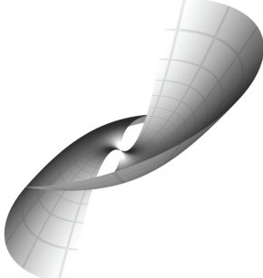
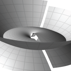
Figure 2. A surface of revolution in $T_{2}$ with timelike axis, a surface in its associate family, and the parallel constant Gaussian curvature surface (left to right). The second and third surfaces appear to have cuspidal edge singularities.

Proof.

Because $B_{0}|_{z=0}=(4ab\lambda^{2}+4b^{2})\cdot I$, we have $B|_{z=0}=F|_{z=0}=I$. We set $\Theta=\Theta_{1}dx+\Theta_{2}dy$, where $z=x+iy$, with

$$\Theta_{1}=\begin{pmatrix}0&\tfrac{2ab}{\lambda v}-\tfrac{v\lambda}{2}\\ \tfrac{2ab\lambda}{v}-\tfrac{v}{2\lambda}&0\end{pmatrix}\;,\hskip 19.91684pt\Theta_{2}=i\begin{pmatrix}-\tfrac{v^{\prime}}{2v}&\tfrac{2ab}{\lambda v}+\tfrac{v\lambda}{2}\\ -\tfrac{2ab\lambda}{v}-\tfrac{v}{2\lambda}&\tfrac{v^{\prime}}{2v}\end{pmatrix}\;.$$

A computation gives $B_{x}+(\Theta_{1}+i\Theta_{2})B=0$ and $\Theta_{2}B-iBA=0$, implying $dB+\Theta B-BA(dx+idy)=0$, and so $F^{-1}dF=\Theta$. Noting that $\Theta_{1}+i\Theta_{2}$ has no singularity at $\lambda=0$, we have that $B$ is holomorphic in $\lambda$ for all $\lambda\in\mathbb{C}$. Also, $\text{trace}(\Theta_{1}+i\Theta_{2})=0$ implies $\det B$ is constant, so $\det B=1$. Hence $B$ takes values in $\widehat{\mathcal{U}}^{\mathbb{C}}_{+}$. We have $\tau(\Theta)=\Theta$, so $\tau(F^{-1}dF)=F^{-1}dF$. It follows from $F|_{z=0}=I$ that $\tau(F)=F$, so $F$ takes values in $\mathcal{U}_{\tau}$. ∎

Remark 5.2.

Note that we must restrict $\kappa_{1},\kappa_{2}$ so that $v$ is never zero on $\Sigma$. When $v$ reaches zero, this is precisely the moment when $\phi$ leaves $\mathcal{B}_{1,1}$. Also, note that $v$ can be non-constant even when $c=0$. A solution to the equation for $v$, for example when $0<b<a$ and $c\leq 0$, is given in terms of the Jacobi sn function as: $v(x)=2b\ell^{-1}\text{sn}_{b/(\ell^{2}a)}(2\ell a(x+x_{0}))$, where $\ell$ is the largest (in absolute value) of the real solutions to the equation $a^{2}\ell^{4}+(c^{2}-a^{2}-b^{2})\ell^{2}+b^{2}=0$, and $x_{0}$ is chosen so that $v(0)=2b$ and $v^{\prime}(0)\geq 0$.

Inserting the above $F$ into the Sym-Bobenko formula, we get explicit parametrizations of CMC rotational surfaces in $\mathbb{R}^{2,1}$. Because the mean curvature $H$ and the Hopf differential term $Q$ are constant reals, and because the metric $ds^{2}$ is invariant under translation of the $z$-plane in the direction of the imaginary axis, we conclude that these surfaces are rotationally symmetric, by the fundamental theorem for surface theory, and we have the following corollary.

Corollary 5.3.

Inserting $F$ as in Theorem 5.1 into (22) with $\lambda_{0}=1$, we have a surface of revolution $\hat{f}^{1}$ with axis parallel to the line through $0$ and $iA$ in $\mathbb{R}^{2,1}\approx\mathfrak{su}_{1,1}$. In particular, the axis is timelike, null or spacelike when $(a+b)^{2}-c^{2}$ is negative, zero or positive, respectively.

Proof.

The rotational symmetry of the surface is represented by $F\to\exp(iy_{0}A)F$ at $\lambda_{0}=1$ for each $y_{0}\in\mathbb{R}$, and the Sym-Bobenko formula changes from $\hat{f}^{1}$ to

$$\exp(iy_{0}A)\hat{f}^{1}\exp(-iy_{0}A)-iH^{-1}\partial_{\lambda}(\exp(iy_{0}A))|_{\lambda=1}\cdot\exp(-iy_{0}A)\;.$$

The axis is then a line parallel to the line invariant under conjugation by $\exp(iy_{0}A)$. ∎

Remark 5.4.

Using conjugation by $\text{diag}(\sqrt{i},1/\sqrt{i})$ on all of $A$, $\phi$, $F$, $B$, one can see that if we choose $H=-2ab$, Equation (20) gives $v=e^{-u}$ and $Q=1$, for the surfaces in Corollary 5.3.

5.2. Equivariant surfaces

By inserting the $F$ in Theorem 5.1 into (22) and evaluating at various values of $\lambda_{0}\in\mathbb{S}^{1}$, we get surfaces in the associate families of the surfaces of revolution in Corollary 5.3. These are the equivariant surfaces, which we now describe.

Definition 5.5.

An immersion $f:U\subset\mathbb{R}^{2}\to{\mathbb{R}^{2,1}}$ is equivariant with respect to $y$ if there exists a continuous homomorphism $R_{t}:\mathbb{R}\to\mathcal{E}$ into the group $\mathcal{E}$ of isometries of ${\mathbb{R}^{2,1}}$ such that

$$f(x,\,y+t)=R_{t}f(x,\,y).$$

In the following we write $z=x+iy$.

Proposition 5.6.

Let $f:U\subset\mathbb{R}^{2}\to{\mathbb{R}^{2,1}}$ be a conformal immersion with metric $4v^{-2}{\lvert dz\rvert}^{2}$, mean curvature $H$, and Hopf differential $Q\,dz^{2}$. Then $f$ is equivariant with respect to $y$ if and only if $v$, $H$ and $Q$ are $y$-independent.

Proof.

The proposition is shown by the following sequence of equivalent statements:

1. The immersion $f$ is equivariant with respect to $y$.

2. For any $t\in\mathbb{R}$, the maps $f(x,\,y)$ and $f_{t}(x,\,y)=f(x,\,y+t)$ differ by an isometry $R_{t}$ of ${\mathbb{R}^{2,1}}$. To show statement 1 from 2, note that $R_{s+t}f(x,\,y)=f(x,\,y+s+t)=R_{t}f(x,\,y+s)=R_{t}R_{s}f(x,\,y)$, so under suitable non-degeneracy conditions on $f$, the map $t\mapsto R_{t}$ is a continuous homomorphism.

3. The immersions $f$ and $f_{t}$ have equal first and second fundamental forms. Statements 2 and 3 are equivalent by the fundamental theorem of surface theory.

4. The geometric data for $f$ satisfy $v(x,\,y+t)=v(x,\,y)$, $H(x,\,y+t)=H(x,y)$ and $Q(x,\,y+t)=Q(x,\,y)$.

5. The functions $v$, $H$ and $Q$ are $y$-independent. ∎

Proposition 5.7.

Let $f:\Sigma\subset\mathbb{C}\to{\mathbb{R}^{2,1}}$ be a conformal CMC $H$ immersion with metric $4v^{-2}{\lvert dz\rvert}^{2}$ and Hopf differential $Q\,dz^{2}$. Take $q\in{\mathbb{R}}^{*}:={\mathbb{R}}\setminus\{0\}$ so that $4H^{2}=q^{2}$, and suppose $|Q|$ is $1$ at some point in $\mathbb{R}^{2}$. Then $f$ is equivariant with respect to $y$ if and only if $Q$ is constant, $v$ depends only on $x$, and for some $p\in\mathbb{R}$, $v$ satisfies

(31) $${v^{\prime}}^{2}=v^{4}-2pv^{2}+q^{2},\quad v^{\prime\prime}=2v(v^{2}-p).$$

Proof.

If $f$ is equivariant, then $v$ and $Q$ are $y$-independent by Proposition 5.6. Since $f$ is CMC, then $Q$ is holomorphic in $z$, and is hence constant. So $|Q|\equiv 1$. Since $v$ is $y$-independent, the Gauss equation (18) with $v=e^{-u}$ is a second order ODE in $x$. Multiplying the Gauss equation by $u^{\prime}$ and integrating yields (31), where $p$ is a constant of integration.

Conversely, if $v$ and $Q$ satisfy the conditions of the proposition, then $f$ is equivariant, by Proposition 5.6. ∎

Corollary 5.8.

Any immersion $\hat{f}^{\lambda_{0}}$ into ${\mathbb{R}^{2,1}}$ as in (22), obtained from a DPW potential of the form $Adz$, where $A$ is given by (30), is a conformal CMC immersion equivariant with respect to $y$.

Conversely, up to an isometry of ${\mathbb{R}^{2,1}}$, every non-totally-umbilic conformal spacelike CMC $H\neq 0$ immersion equivariant with respect to $y$ is obtained from some DPW potential $Adz$, where $A$ is of the form (30).

Proof.

By Theorem 5.1, the extended frame of the immersion obtained from $A$ is of the form $F(x,\,y)=\exp(iyA)\mathcal{G}(x)$ for some map $\mathcal{G}:J\to SU_{1,1}$, where $J=(-\kappa_{1}^{2},\kappa_{2}^{2})\subset{\mathbb{R}}$. The Sym-Bobenko formula $\hat{f}^{\lambda_{0}}$ applied to $F$ yields an immersion which is equivariant with respect to $y$.

Conversely, given a CMC immersion $f:(-\tilde{\kappa}_{1}^{2},\tilde{\kappa}_{2}^{2})\times{\mathbb{R}}\subset\mathbb{R}^{2}\to{\mathbb{R}^{2,1}}$, which is equivariant with respect to the second coordinate $y$, let $4v^{-2}{\lvert dz\rvert}^{2}$ and $Qdz^{2}$ be the metric and Hopf differential for $f$, respectively. By a dilation of coordinates $z\to rz$ for a constant $r\in\mathbb{R}$, we may assume $|Q|=1$. Let $q$ be as in Proposition 5.7. By that proposition, $v$ satisfies (31) for some $p\in\mathbb{R}$. Let $b=v(0)/2$, and define $a\in{\mathbb{R}}^{*}$ by the equation $H=-2ab$, and so $q=\pm 4ab$. Then it follows that $p\leq 2(a^{2}+b^{2})$, and there exist $c\in\mathbb{R}$ and $\lambda_{0}\in\mathbb{S}^{1}$ such that $p=2(a^{2}+b^{2}-c^{2})$ and $Q=\lambda_{0}^{-2}$. Let $\hat{f}^{\lambda_{0}}$ be the immersion induced from the DPW potential $\xi=A\textup{d}z$, with $A$ as in Theorem 5.1, initial condition $\Phi(0)=I$, and $\lambda_{0}$ and $H=-2ab$. Then $\hat{f}^{\lambda_{0}}$ has metric $4v^{-2}{\lvert dz\rvert}^{2}$, by Theorems 5.1 and 3.8, and has mean curvature $-2ab$ and Hopf differential $\lambda_{0}^{-2}dz^{2}$. By the fundamental theorem of surface theory, $f$ and $\hat{f}^{\lambda_{0}}$ differ by an isometry of ${\mathbb{R}^{2,1}}$. ∎

We now describe the two spaces $R/\!\!\sim_{R}$ and $E/\!\!\sim_{E}$ of immersions into ${\mathbb{R}^{2,1}}$ which are rotationally invariant and equivariant, respectively. Both constructions are based on the family of solutions to the integrated Gauss equation (31), where solutions are identified which amount to a coordinate shift and hence yield ambiently isometric immersions. Bifurcations in the space of solutions to Equation (31) lead to non-Hausdorff quotient spaces.

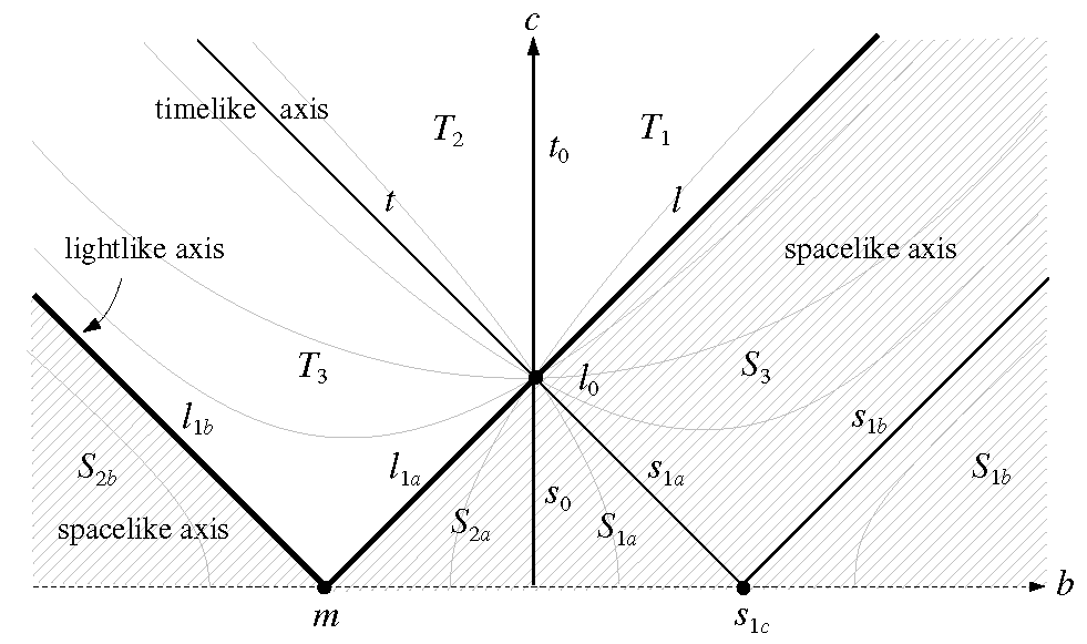
Figure 3. A blowup of the moduli space of surfaces with rotational symmetry $\mathbb{R}^{2,1}$. The blowdown is obtained by identifying points along segments of hyperbolas within each region. The heavily drawn left v-shaped line represents the lightlike axis examples, separating those with spacelike and timelike axes. The line segments and points in the diagram represent examples whose metrics degenerate to elementary functions; in particular, the $c$-axis represents hyperboloids. Pairs in the same associate family are represented by points reflected across the $c$-axis.

The space $R/\!\!\sim_{R}$ of immersions with rotational symmetry is a quotient of the space

$$R=\{(p,\,q,\,v_{0})\in\mathbb{R}^{3}~{}|~{}v_{0}^{4}-2pv_{0}^{2}+q^{2}\geq 0\}$$

parametrizing solutions to (31). The equivalence relation $\sim_{R}$ on $R$ is defined as follows: $(p_{1},\,q_{1},\,v_{1})\!\!\sim_{R}\!\!(p_{2},\,q_{2},\,v_{2})$ if, for $k=1$ and $2$, the respective solutions to

(32) $$\begin{split}&{v^{\prime}}^{2}=v^{4}-2p_{k}v^{2}+q_{k}^{2},\\ &v^{\prime\prime}=2v(v^{2}-p_{k}),\\ &v(0)=v_{k},\end{split}$$

are equivalent in the following sense: there exist $r\in\mathbb{R}_{+}$ and $c\in\mathbb{R}$ such that $v_{2}(x)=rv_{1}(rx+c)$ or $v_{2}(x)=-rv_{1}(rx+c)$. The space $R/\!\!\sim_{R}$ is a $1$-dimensional non-Hausdorff manifold. For a point in $R$ with $q\neq 0$, the corresponding surface is constructed by relating (32) to (29). This determines $a$, $b$ and $c$ in Theorem 5.1, and the surface is given by Corollary 5.3. If $q=0$, the surface is totally umbilic.

To describe the space of equivariant immersions, let

$$E=\{(p,\,P,\,v_{0})\in\mathbb{R}\times\mathbb{C}\times\mathbb{R}~{}|~{}v_{0}^{4}-2pv_{0}^{2}+{\lvert P\rvert}^{2}\geq 0\}.$$

The equivalence relation $\sim_{E}$ on $E$ is defined as follows: $(p,\,P,\,v_{0})\!\!\sim_{E}\!\!(p^{\prime},\,P^{\prime},\,v_{0}^{\prime})$ if there exist $q,\,q^{\prime}\in\mathbb{R}$ and $\lambda\in\mathbb{S}^{1}$ such that $P=q\lambda^{-2}$ and $P^{\prime}=q^{\prime}\lambda^{-2}$, and $(p,\,q,\,v_{0})\!\!\sim_{R}\!\!(p^{\prime},\,q^{\prime},\,v_{0}^{\prime})$. The space $E/\!\!\sim_{E}$ is a $2$-dimensional non-Hausdorff manifold. The surface corresponding to a point in $E$, when $P\neq 0$, is as in the case of the space $R$, except that the Sym-Bobenko formula now uses general $\lambda\in\mathbb{S}^{1}$ (not necessarily $\lambda=1$). When $P=0$, the surface is totally umbilic.

The above constructions are summarized as:

Theorem 5.9.

Up to coordinate change and ambient isometry, the spaces $E/\!\!\sim_{E}$ and $R/\!\!\sim_{R}$ are the moduli spaces of CMC immersions into ${\mathbb{R}^{2,1}}$ which are respectively equivariant and rotational.

5.3. The moduli space of surfaces with rotational symmetry

Figure 3 shows a blowup of the moduli space of surfaces with rotational symmetry in ${\mathbb{R}^{2,1}}$. The underlying space is the closed $(b,c)$-half-plane obtained by the normalization $\lambda=1$ and $a=1$. The blowdown to the 1-dimensional moduli space of surfaces is the quotient modulo identification of points on segments of hyperbolas $1+b^{2}-c^{2}=(\mathrm{constant})\cdot b$ foliating each region. The examples with spacelike, timelike and lightlike axes are represented respectively by the shaded and unshaded regions, and the left heavily-drawn v-shaped line. Subscripted letters $S$, $L$ and $T$ denote one-parameter families with spacelike, lightlike and timelike axes, respectively; likewise, $s$, $\ell$ and $t$ designate single examples, and the example $m$ has no axis. The moduli space is a connected non-Hausdorff space, and is the disjoint union of eight one-parameter families $S_{1a}$, $S_{1b}$, $S_{2a}$, $S_{2b}$, $S_{3}$, $T_{1}$, $T_{2}$, $T_{3}$, eight individual examples $s_{1a}$, $s_{1b}$, $s_{1c}$, $\ell_{1a}$, $\ell_{1b}$, $m$, $\ell$, $t$, and the hyperboloids corresponding to $s_{0}$, $\ell_{0}$, $t_{0}$ considered with spacelike, lightlike and timelike axes respectively.

The non-Hausdorffness of the moduli space arises from the fact that the limit surface of a sequence of surfaces in any of the one-parameter families (designated by capital letters) to a point not in that family is not uniquely determined: the sequence will have different limit surfaces depending on how the sequence is chosen to be positioned in ${\mathbb{R}^{2,1}}$. The blowup of the moduli space shown in Figure 3 maps this topology. For example, the same sequence of surfaces in $S_{3}$ can converge to either $s_{1a}$, $s_{1b}$ or $s_{1c}$; likewise a sequence in $T_{3}$ can converge to either $l_{1a}$, $l_{1b}$ or $m$.

$\begin{array}[]{cccc}\includegraphics[width=85.35826pt]{minkowski_delaunay_S1a.png}&\includegraphics[width=85.35826pt]{minkowski_delaunay_S1b.png}&\includegraphics[width=85.35826pt]{minkowski_delaunay_S2a.png}&\includegraphics[width=85.35826pt]{minkowski_delaunay_S2b.png}\\ \text{\footnotesize$S_{1a}$ ($\frac{1}{2}$,\,$0$)}&\text{\footnotesize$S_{1b}$ ($2$,\,$0$)}&\text{\footnotesize$S_{2a}$ ($-\frac{1}{2}$,\,$0$)}&\text{\footnotesize$S_{2b}$ ($-2$,\,$0$)}\vspace{2ex}\\ \includegraphics[width=85.35826pt]{minkowski_delaunay_S3.png}&\includegraphics[width=85.35826pt]{minkowski_delaunay_T1.png}&\includegraphics[width=85.35826pt]{minkowski_delaunay_T2.png}&\includegraphics[width=85.35826pt]{minkowski_delaunay_T3.png}\\ \text{\footnotesize$S_{3}$ ($1$,\,$\sqrt{2}$)}&\text{\footnotesize$T_{1}$ ($1$,\,$4$)}&\text{\footnotesize$T_{2}$ ($-1$,\,$4$)}&\text{\footnotesize$T_{3}$ ($-1$,\,$\sqrt{2}$)}\end{array}$

Figure 4. Examples from each of the eight families of surfaces with rotational symmetry in ${\mathbb{R}^{2,1}}$. These families together with the eight single examples shown in Figure 5 comprise all such surfaces. The designation symbol and the numbers $(b,\,c)$ refer to the blowup of the moduli space in Figure 3. Note that entire examples are necessarily complete [10]. Images created with XLab [28].

$\begin{array}[]{cccc}\includegraphics[width=85.35826pt]{minkowski_delaunay_ss1a.png}&\includegraphics[width=85.35826pt]{minkowski_delaunay_ss1b.png}&\includegraphics[width=85.35826pt]{minkowski_delaunay_t.png}&\includegraphics[width=85.35826pt]{minkowski_delaunay_l.png}\\ \text{\footnotesize$s_{1a}$ ($\frac{1}{2}$,\,$\frac{1}{2}$)}&\text{\footnotesize$s_{1b}$ ($2$,\,$1$)}&\text{\footnotesize$t$ ($-1$,\,$2$)}&\text{\footnotesize$\ell$ ($1$,\,$2$)}\\ \includegraphics[width=85.35826pt]{minkowski_delaunay_l1a.png}&\includegraphics[width=85.35826pt]{minkowski_delaunay_l1b.png}&\includegraphics[width=85.35826pt]{minkowski_delaunay_s1c.png}&\includegraphics[width=85.35826pt]{minkowski_delaunay_s0.png}\\ \text{\footnotesize$\ell_{1a}$ ($-\frac{1}{2}$,\,$\frac{1}{2}$)}&\text{\footnotesize$\ell_{1b}$ ($-2$,\,$1$)}&s_{1c},\,m&s_{0},\,\ell_{0},\,t_{0}\vspace{2ex}\end{array}$

Figure 5. The eight surfaces with rotational symmetry in ${\mathbb{R}^{2,1}}$ whose metric is an elementary function. The last two examples, a cylinder over a hyperbola and a hyperboloid respectively, appear multiple times in the blowup of the moduli space. Designation symbols are as in Figure 3. Images created with XLab [28].

6. Analogues of Smyth surfaces in $\mathbb{R}^{2,1}$

A generalization of Delaunay surfaces in $\mathbb{R}^{3}$ was studied by B. Smyth in [31]. These are constant mean curvature surfaces whose metrics are invariant under rotations. They were also studied by Timmreck et al. in [33], where they were shown to be properly immersed (a property which we will see does not hold for the analogue in ${\mathbb{R}}^{2,1}$). The DPW approach was applied in [14] and [8].

Here we use the DPW method to construct the analogue of Smyth surfaces in $\mathbb{R}^{2,1}$, and describe some of their properties. Define

(33) $$\xi=\lambda^{-1}\begin{pmatrix}0&1\\ cz^{k}&0\end{pmatrix}dz\;,\;\;\;c\in\mathbb{C}\;,\;\;\;z\in\Sigma=\mathbb{C}\;,$$

and take the solution $\phi$ of $d\phi=\phi\xi$ with $\phi|_{z=0}=I$. If $k=0$ and $c\in\mathbb{S}^{1}$, then one can explicitly split $\phi$ as in Example 3.10, and the resulting CMC surface is a cylinder over a hyperbola whose axis depends on the choice of $c$. When $c=0$, one produces a two-sheeted hyperboloid. However, when $c\not\in\mathbb{S}^{1}\cup\{0\}$ or when $k>0$, Iwasawa splitting of $\phi$ is not so simple.

Changing $c$ to $ce^{i\theta_{0}}$ for any $\theta_{0}\in\mathbb{R}$ only changes the resulting surface by a rigid motion and a reparametrization $z\to ze^{-\frac{i\theta_{0}}{k+2}}$. So without loss of generality we assume that $c\in\mathbb{R}^{+}:={\mathbb{R}}\cap(0,\infty)$.

Lemma 6.1.

The surfaces $f:\Sigma^{\circ}=\phi^{-1}(\mathcal{B}_{1,1})\to{\mathbb{R}}^{2,1}$, produced via the DPW method, from $\xi$ in (33), with $\phi|_{z=0}=I$ and $\lambda_{0}=1$, have reflective symmetry with respect to $k+2$ geodesic planes that meet equiangularly along a geodesic line.

Proof.

Consider the reflections

$$R_{\ell}(z)=e^{\frac{2\pi i\ell}{k+2}}\bar{z},$$

of the domain $\Sigma=\mathbb{C}$, for $\ell\in\{0,1,...,k+1\}$. In the coordinate $w:=R_{\ell}(z)$, we have

$$\xi=A_{\ell}\Big{(}\lambda^{-1}\begin{pmatrix}0&1\\ c\bar{w}^{k}&0\end{pmatrix}\textup{d}\bar{w}\Big{)}A_{\ell}^{-1},\hskip 28.45274ptA_{\ell}=\text{diag}(e^{\frac{\pi i\ell}{k+2}},e^{\frac{-\pi i\ell}{k+2}}).$$

Comparing this with (33), it follows that $\phi(z)=A_{\ell}\phi(\bar{w})A_{\ell}^{-1}$, and hence

$$\phi(R_{\ell}(z))=A_{\ell}\phi(\bar{z})A_{\ell}^{-1}.$$

It is easy to see that this relation extends to the factors $F$ and $B$ in the Iwasawa splitting $\phi=FB$, and so we have a frame $F$ which satisfies

$$F(R_{\ell}(z))=A_{\ell}F(\bar{z})A_{\ell}^{-1}.$$

Since we have assumed $c\in{\mathbb{R}}^{+}$, it follows from the form of $\xi$ and the initial condition for $\phi$ that $\phi(\bar{z},\lambda)=\overline{\phi(z,\bar{\lambda})}$. This symmetry also extends to the factors $F$ and $B$, and combines with the first symmetry as: $F(R_{\ell}(z),\lambda)=A_{\ell}\overline{F(z,\bar{\lambda})}A_{\ell}^{-1}$. Inserting this into (22), we have

$$\hat{f}^{\lambda}(R_{\ell}(z))=-A_{\ell}\overline{\hat{f}^{\bar{\lambda}}(z)}A_{\ell}^{-1}\;.$$

Then for $\hat{f}^{1}$, the transformation $\hat{f}^{1}\to-\overline{\hat{f}^{1}}$ represents reflection across the plane $\{x_{2}=0\}$ of $\mathbb{R}^{2,1}=\{x_{1}e_{1}+x_{2}e_{2}+x_{0}e_{3}\}$, and conjugation by $A_{\ell}$ represents a rotation by angle $2\pi i\ell/(k+2)$ about the $x_{0}$-axis. ∎

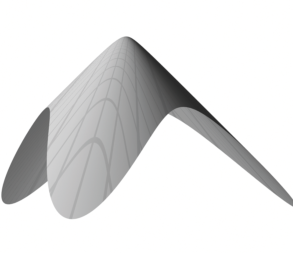
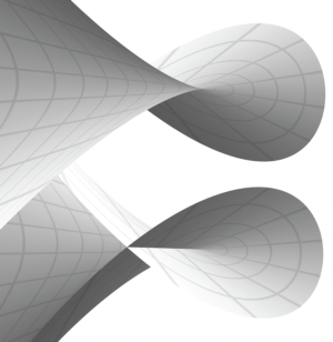
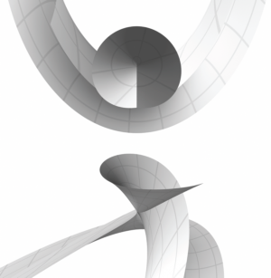
Figure 6. Details of Smyth surface analogs in $\mathbb{R}^{2,1}$. An immersed portion of this surface (left) has three-fold ambient rotational symmetry, Lemma 6.1. A singularity further out on the surface appears to be a swallowtail (second image). The third image shows another singularity on the same surface.

We now show that $u:\Sigma^{\circ}\to\mathbb{R}$ in the metric (16) of the surface resulting from the frame $F$ is constant on each circle of radius $r$ centered at the origin in $\Sigma$, that is, $u=u(r)$ is independent of $\theta$ in $z=re^{i\theta}$. Having this internal rotational symmetry of the metric (without actually having a surface of revolution) is what defines the surface as an analogue of a Smyth surface.

Proposition 6.2.

The solution $u$ of the Gauss equation (18) for a surface generated by $\xi$ in (33), with $\phi|_{z=0}=I$, is rotationally symmetric. That is, $u$ depends only on $|z|$.

Proof.

Define

$$\tilde{z}=e^{i\theta}z,\hskip 28.45274pt\tilde{\lambda}=e^{i\theta}e^{\frac{i\theta k}{2}}\lambda,$$

for any fixed $\theta\in{\mathbb{R}}$. Then

$$\xi(z,\lambda)=L^{-1}\,\Big{(}\tilde{\lambda}^{-1}\begin{pmatrix}0&1\\ c\tilde{z}^{k}&0\end{pmatrix}\textup{d}\tilde{z}\Big{)}\,L,\hskip 28.45274ptL=\begin{pmatrix}e^{\frac{-ik\theta}{4}}&0\\ 0&e^{\frac{ik\theta}{4}}\end{pmatrix}.$$

It follows that

$$\phi(\tilde{z},\tilde{\lambda})=L\,\phi(z,\lambda)\,L^{-1}.$$

Let $\phi=FB$ be the normalized Iwasawa splitting of $\phi$, with $B:\Sigma^{\circ}\to\widehat{\mathcal{U}}^{\mathbb{C}}_{+}$. Then

$$\phi(\tilde{z},\tilde{\lambda}) = (LF(z,\lambda)L^{-1})\cdot(LB(z,\lambda)L^{-1})$$

$$= F(\tilde{z},\tilde{\lambda})\cdot B(\tilde{z},\tilde{\lambda}).$$

Since $LB(z,\lambda)L^{-1}$ and $B(\tilde{z},\tilde{\lambda})$ are both loops in $\widehat{\mathcal{U}}^{\mathbb{C}}_{+}$, and the left factors are both loops in $\mathcal{U}$, it follows by uniqueness that the corresponding factors are equal. Recall from Section 3.4 that $u=2\log\rho$ is determined by the function $\rho(z)$, which is the first component of the diagonal matrix $B(z)\big{|}_{\lambda=0}$. Since this matrix is diagonal and independent of $\lambda$, we have just shown that $B(z)\big{|}_{\lambda=0}=B(\tilde{z})\big{|}_{\lambda=0}$, and hence $u(\tilde{z})=u(z)$. ∎

We now show that the Gauss equation for these surfaces in $\mathbb{R}^{2,1}$ is a special case of the Painleve III equation. This was proven for Smyth surfaces in $\mathbb{R}^{3}$, in [8].

Proposition 6.3.

The Gauss equation (18) for a surface generated by $\xi$ in (33), with $\phi|_{z=0}=I$, is a special case of the Painleve III equation.

Proof.

The Painleve III equation, for constants $\alpha,\beta,\gamma,\delta$, is

$$y^{\prime\prime}=y^{-1}(y^{\prime})^{2}-x^{-1}y^{\prime}+x^{-1}(\alpha y^{2}+\beta)+\gamma y^{3}+\delta y^{-1},$$

where $\prime$ denotes the derivative with respect to $x$. Setting $y=e^{v}$, $\alpha=\beta=0$, $\gamma=-\delta=1$, we have $(v^{\prime}e^{v})^{\prime}=e^{-v}{(v^{\prime}e^{v})}^{2}-x^{-1}v^{\prime}e^{v}+0+e^{3v}-e^{-v}$. Therefore

(34) $$v^{\prime\prime}+x^{-1}v^{\prime}-2\sinh(2v)=0$$

is a particular case of the Painleve III equation.

By a homothety and/or reflection, we may assume the surface has $H=1/2$, and then we have $Q=-cz^{k}$. (By Section 3.4, $Q=-2Hb_{-1}/a_{-1}$.) Setting $r:=|z|$, the Gauss equation becomes

(35) $$4u_{z\bar{z}}+c^{2}\,r^{2k}e^{-2u}-e^{2u}=0\;.$$

To prove this proposition, we show that Equation (35) can be written in the form (34). Set

$$v:=u-\tfrac{1}{2}\log|Q|=u-\tfrac{1}{2}\log c-\tfrac{k}{2}\log r\;,$$

so $4v_{z\bar{z}}+\tfrac{k}{2}(\log r)_{z\bar{z}}+c^{2}\,r^{2k}\,e^{-2(v+\frac{1}{2}\log c+\frac{k}{2}\log{r})}-e^{2(v+\frac{1}{2}\log c+\frac{k}{2}\log{r})}=0$, and this simplifies to

$$4v_{z\bar{z}}-2c\,r^{k}\,\sinh(2v)=0.$$

Now $v$ is a function of $r$ only, which means that $v_{z\bar{z}}=\frac{1}{4}(v^{\prime\prime}(r)+\frac{1}{r}v^{\prime}(r))$, and the equation becomes

$$v^{\prime\prime}(r)+r^{-1}v^{\prime}(r)-2c\,r^{k}\,\sinh(2v)=0.$$

Now set

$$\mu:=(1+\frac{k}{2})^{-1}r^{1+\frac{k}{2}}\,\sqrt{c}.$$

Then $\partial_{r}\mu=r^{\frac{k}{2}}\,\sqrt{c}$. So we have

$$\partial_{r}(\partial_{\mu}v\,r^{\frac{k}{2}}\sqrt{c})+r^{-1}\partial_{\mu}v\,r^{\frac{k}{2}}\sqrt{c}-2c\,r^{k}\,\sinh(2v)=0\;,$$

which simplifies to $v_{\mu\mu}+\mu^{-1}\,v_{\mu}-2\sinh(2v)=0$, coinciding with (34). ∎

References

• [1] K Akutagawa and S Nishikawa, The Gauss map and spacelike surfaces with prescribed mean curvature in Minkowski 3-space, Tohoku Math. J. (2) 42 (1990), 67–82.
• [2] V Balan and J Dorfmeister, Birkhoff decompositions and Iwasawa decompositions for loop groups, Tohoku Math. J. 53 (2001), 593–615.
• [3] R Bartnik, Regularity of variational maximal surfaces, Acta Math. 161 (1988), 145–181.
• [4] R Bartnik and L Simon, Spacelike hypersurfaces with prescribed boundary values and mean curvature, Commun. Math. Phys. 87 (1982), 131–152.
• [5] A I Bobenko, All constant mean curvature tori in ${R}^{3}$, ${S}^{3}$, ${H}^{3}$ in terms of theta-functions, Math. Ann. 290 (1991), 209–245.
• [6] by same author, Constant mean curvature surfaces and integrable equations, Uspekhi Mat. Nauk 46:4 (1991), 3–42. English translation in: Russian Math. Surveys, 46 (1991), 1-45.
• [7] by same author, Surfaces in terms of 2 by 2 matrices. Old and new integrable cases, Harmonic maps and integrable systems, Aspects of Mathematics, no. E23, Vieweg, 1994.
• [8] A I Bobenko and A Its, The Painleve III equation and the Iwasawa decomposition, Manuscripta Math. 87 (1995), 369–377.
• [9] L Bungart, On analytic fiber bundles, Topology 7 (1968), 55–68.
• [10] S Y Cheng and S T Yau, Maximal space-like hypersurfaces in the Lorentz-Minkowski spaces, Ann. of Math. 104 (1976), 407–419.
• [11] H Y Choi and A Treibergs, Gauss maps of spacelike constant mean curvature hypersurfaces of Minkowski space, J. Differential Geom. 32 (1990), no. 3, 775–817.
• [12] J Dorfmeister and G Haak, On symmetries of constant mean curvature surfaces. I. General theory, Tohoku Math. J. (2) 50 (1998), 437–454.
• [13] by same author, Construction of non-simply connected CMC surfaces via dressing, J. Math. Soc. Japan 55 (2003), no. 2, 335–364.
• [14] J Dorfmeister, F Pedit and H Wu, Weierstrass type representation of harmonic maps into symmetric spaces, Comm. Anal. Geom. 6 (1998), 633–668.
• [15] H Grauert and R Remmert, Theory of Stein spaces, Springer-Verlag, 1979.
• [16] M A Guest, Harmonic maps, loop groups, and integrable systems, London Mathematical Society Student Texts, vol. 38, Cambridge University Press, 1997.
• [17] J Hano and K Nomizu, Surfaces of revolution with constant mean curvature in Lorentz-Minkowski space, Tohoku Math. J. (2) 36 (1984), no. 3, 427–437.
• [18] J Inoguchi, Surfaces in Minkowski 3-space and harmonic maps, Harmonic morphisms, harmonic maps, and related topics (Brest, 1997), 249–270, Chapman & Hall/CRC Res. Notes Math., 413, Chapman & Hall/CRC, Boca Raton, FL, 2000.
• [19] T Ishihara and F Hara, Surfaces of revolution in the Lorentzian $3$-space, J. Math Tokushima Univ. 22 (1989), 1–13.
• [20] P Kellersch, Eine Verallgemeinerung der Iwasawa Zerlegung in Loop Gruppen, PhD Thesis, TU Munich, 1999.
• [21] K Kenmotsu, Weierstrass formula for surfaces of prescribed mean curvature, Math. Ann. 245 (1979), 89–99.
• [22] M Kilian, S-P Kobayashi, W Rossman and N Schmitt, Constant mean curvature surfaces of any positive genus, J. Lond. Math. Soc. 72 (2005), 258–272.
• [23] M Kilian, I McIntosh and N Schmitt, New constant mean curvature surfaces, J. Exp. Math. 9 (2000), 595–611.
• [24] T K Milnor, Harmonic maps and classical surface theory in Minkowski 3-space, Trans. Amer. Math. Soc. 208 (1983), 161–185.
• [25] U Pinkall and I Sterling, On the classification of constant mean curvature tori, Ann. of Math. (2) 130 (1989), 407–451.
• [26] K Pohlmeyer, Integrable Hamiltonian systems and interactions through quadratic constraints, Comm. Math. Phys. 46 (1976), no. 3, 207–221.
• [27] A Pressley and G Segal, Loop groups, Oxford Math. monographs, Clarendon Press, Oxford, 1986.
• [28] N Schmitt, XLab, software.
• [29] N Schmitt, M Kilian, S-P Kobayashi and W Rossman, Unitarization of monodromy representations and constant mean curvature trinoids in 3-dimensional space forms, J. Lond. Math. Soc. (2) 75 (2007), no. 3, 563–581.
• [30] O Shcherbak, Wave fronts and reflection groups, Uspekhi Mat. Nauk 43 (1988), no. 3(261), 125–160. English translation in: Russian Math. Surveys 43 (1988), no. 3, 149–194.
• [31] B Smyth, A generalization of a theorem of Delaunay on constant mean curvature surfaces, IMA Vol. Math. Appl 51 (1993), 123–130.
• [32] A Sym, Soliton surfaces and their applications, Geometric aspects of the Einstein equations and integrable systems, Lecture notes in Physics, vol. 239, Springer, 1985, pp. 154–231.
• [33] M Timmreck, U Pinkall and D Ferus, Constant mean curvature planes with inner rotational symmetry in Euclidean $3$-space, Math. Z. 215 (1994), 561–568.
• [34] A Treibergs, Entire spacelike hypersurfaces of constant mean curvature in Minkowski space, Ann. of Math. Stud. (1982), no. 102, 229–238, Seminar on Differential Geometry.
• [35] K Uhlenbeck, Harmonic maps into Lie groups: classical solutions of the chiral model, J. Differential Geom. 30 (1989), 1–50.
• [36] T Y H Wan, Constant mean curvature surface, harmonic maps, and universal Teichmüller space, J. Diff. Geom. 35 (1992), 643–657.
• [37] T Y H Wan and T K K Au, Parabolic constant mean curvature spacelike surfaces, Proc. Amer. Math. Soc. 120, (1994), 559–564.