Pair Analysis of Field Galaxies from the Red-Sequence Cluster Survey

Abstract

We study the evolution of the number of close companions of similar luminosities per galaxy ($N_{c}$) by choosing a volume-limited subset of the photometric redshift catalog from the Red-Sequence Cluster Survey (RCS-1). The sample contains over 157,000 objects with a moderate redshift range of $0.25\leq z\leq 0.8$ and $M_{R_{c}}\leq-20$. This is the largest sample used for pair evolution analysis, providing data over 9 redshift bins with about 17,500 galaxies in each. After applying incompleteness and projection corrections, $N_{c}$ shows a clear evolution with redshift. The $N_{c}$ value for the whole sample grows with redshift as $(1+z)^{m}$, where $m=2.83\pm 0.33$ in good agreement with $N$-body simulations in a $\Lambda$CDM cosmology. We also separate the sample into two different absolute magnitude bins: $-25\leq M_{R_{c}}\leq-21$ and $-21<M_{R_{c}}\leq-20$, and find that the brighter the absolute magnitude, the smaller the $m$ value. Furthermore, we study the evolution of the pair fraction for different projected separation bins and different luminosities. We find that the $m$ value becomes smaller for larger separation, and the pair fraction for the fainter luminosity bin has stronger evolution. We derive the major merger remnant fraction $f_{rem}=0.06$, which implies that about 6% of galaxies with $-25\leq M_{R_{c}}\leq-20$ have undergone major mergers since $z=0.8$.

1 Introduction

Galaxy interactions and mergers play a very important role in the evolution and properties of galaxies. Although mergers are rare in the local universe, a high merger rate in the past can change the morphology, luminosity, stellar population, and number density of galaxies dramatically. The evolution of the merger rate is directly connected to galaxy formation and structure formation in the Universe. Therefore, the measurement of merger rates for galaxies at different merging stages provides important information in the interpretation for various phenomena, such as galaxy and quasar evolution. There are many stages of mergers: close but well-separated galaxies (early-stage mergers), strongly interacting galaxies, and galaxies with double cores (late-stage mergers). Measuring the morphological distortion of galaxies (e.g., Le Févre et al., 2000; Reshetnikov, 2000; Conselice et al., 2003; Lavery et al., 2004; Lotz et al., 2006), as well as studying the spatially resolved dynamics of galaxies (e.g., Puech et al., 2007a, b) are definitive methods for studying on-going mergers, However, they are challenging to observe at high redshift and difficult to quantify. Instead of directly studying on-going mergers, close pairs are much easier to observe and are still able to provide statistical information on the merger rate. A close pair is defined as two galaxies which have a projected separation smaller than a certain distance. Without redshift measurements, a close pair could be just an optical pair, which contains two unrelated galaxies with small separation in angular projection. With spectroscopic redshift measurements, a physical pair can be picked out by choosing two galaxies with similar redshifts and small projected separation. We note that only a fraction of physical pairs are real pairs, which have true physical separations between galaxies smaller than the chosen separation, and are going to merge is a relatively short timescale. Nevertheless, studying any kind of close pairs allows us to glean statistical information on the merger rate.

From $\Lambda$ cold dark matter ($\Lambda$CDM) $N$-body simulations (Governato et al., 1999; Gottlöber et al., 2001), it is found that the merger rates of halos increases with redshift as $(1+z)^{m}$, where $2.5\leq m\leq 3.5$. However, observational pair results produce diverse results of $0\leq m\leq 4$ (e.g., Zepf & Koo, 1989; Burkey et al., 1994; Carlberg, Pritchet & Infante, 1994; Woods et al., 1995; Yee & Ellingson, 1995; Patton et al., 1997; Neuschaefer et al., 1997; Le Févre et al., 2000; Carlberg et al., 2000; Patton et al., 2000, 2002; Bundy et al., 2004; Lin et al., 2004; Cassata et al., 2005; Bridge et al., 2007; Kartaltepe et al., 2007). Often, there are only a few hundred objects in these samples because most studies use spectroscopic redshift data, so that the error bars on the number of pairs are very large. Kartaltepe et al. (2007) utilized a photometric redshift database and included 59,221 galaxies in their sample to perform the pair analysis. The large sample makes their result robust. However, a pair study with a 2 deg² field could still be affected by cosmic variance ($\sim 30$ Mpc $\times$ 30 Mpc at $z=0.5$). Furthermore, some studies use morphological methods to identify pairs on optical images; some close pairs they find could just be late-type galaxies with starburst regions because they have double or triple cores and look asymmetrical. Therefore, the merger rates could be over-estimated. In contrast, other observations have yielded results with no strong evolution at high redshift (e.g., Bundy et al., 2004; Lin et al., 2004). Bundy et al. (2004) also use a morphological method to identify pairs. However, they use near-IR images which reveal real stellar mass distributions and are insensitive to starburst regions. No matter what these previous studies conclude about pair fractions, their results are obtained over a small number of redshift bins and have large error bars due to an inadequate number of objects (with the exception of Kartaltepe et al., 2007). Furthermore, none of these previous studies separate their sample into field and cluster environments. The evolution of the pair fraction can be very different in different environments. The dynamics of galaxy in clusters is also very different compared to that in field; hence, these studies could choose pairs with different properties even using exactly the same pair criteria.

In this paper, a subset of the photometric redshift catalog from Hsieh et al. (2005) is used to investigate the evolution of close galaxy pair fraction. The catalog is created using photometry in $z^{\prime},R_{c},V$, and $B$ from the Red-Sequence Cluster Survey (RCS; Gladders & Yee, 2005). The sky coverage is approximately 33.6 deg². The large sample of photometric redshifts allows us to perform a pair analysis with good statistics. We use about 160,000 galaxies in our sample for the primary galaxies, with a moderate redshift range of $0.25\leq z\leq 0.8$ and $M_{R_{c}}\leq-20$, allowing us to derive very robust results with relatively small error bars.

This paper is structured as follows. In §2 we briefly describe the RCS survey and the photometric redshift catalog used in our analysis. In §3 we provide a description of the sampling criteria for this study. Section 4 presents the method of the pair analysis and the definition of a pair. We describe the selection effects and the methods dealing with the projection effects and incompleteness in §5. The error estimation of the pair fraction is discussed in §6. We then present the results in §7 and discuss the implications of the pair statistics in our data in §8. In §9 we summarize our results and discuss future work. The cosmological parameters used in this study are $\Omega_{\Lambda}=0.7$, $\Omega_{M}=0.3$, $H_{0}=70$ km s^-1Mpc^-1, and $w=-1$.

2 The RCS Survey and Photometric Redshift Catalog

The RCS (Gladders & Yee, 2005) is an imaging survey covering $\sim 92$ deg² in the $z^{\prime}$ and $R_{c}$ bands carried out using the CFH12K CCD camera on the 3.6m Canada-France-Hawaii Telescope (CFHT) for the northern sky, and the Mosaic II camera on the Cerro Tololo Inter-American Observatory (CTIO) 4m Blanco telescope for the southern sky, to search for galaxy clusters in the redshift range of $z<1.4$. Follow-up observations in $V$ and $B$ were obtained using the CFH12K camera, covering 33.6 deg² ($\sim$ 75% complete for the original CFHT RCS fields).

The CFH12K camera is a 12k $\times$ 8k pixel² CCD mosaic camera, consisting of twelve 2k $\times$ 4k pixel² CCDs. It covers a 42 $\times$ 28 arcminute² area for the whole mosaic at prime focus (f/4.18), corresponding to 0”.2059 pixel^-1. For the CFHT RCS runs, the typical seeing was 0.62 arcsec for $z^{\prime}$ and 0.70 arcsec for $R_{c}$. The integration times were typically 1200s for $z^{\prime}$ and 900s for $R_{c}$, with average $5\sigma$ limiting magnitudes of $z^{\prime}_{AB}=23.9$ and $R_{c}=25.0$ (Vega) for point sources. The observations, data, and the photometric techniques, including object finding, photometric measurement, and star-galaxy classification, are described in detail in Gladders & Yee (2005). For the follow-up CFHT RCS observations, the typical seeing was 0.65 arcsec for $V$ and 0.95 arcsec for $B$. The average exposure times for $V$ and $B$ were 480s and 840s, respectively, and the median $5\sigma$ limiting magnitudes (Vega) for point sources are 24.5 and 25.0, respectively. The observations and data reduction techniques are described in detail in Hsieh et al. (2005).

With the four-color ($z^{\prime},R_{c},V,$ and $B$) data, a multi-band RCS photometry catalog covering 33.6 deg² is generated. Although the photometric calibration has been done for all the filters (Gladders & Yee, 2005; Hsieh et al., 2005), we refine the calibration procedure to achieve a better photometric accuracy for this paper. First, we calibrate the patch-to-patch zeropoints for $R_{c}$ by comparing the $R_{c}$ photometry of stars to that in the SDSS DR5 database . We use the empirical transformation function between SDSS filter system and $R_{c}$ determined by Lupton (2005) . The average photometry difference in each patch is the offset we apply. However, patches 0351 and 2153 have no overlapping region with the SDSS DR5. For these two patches, we use the galaxy counts to match their zeropoints to the other patches. The patch-to-patch zeropoint calibration of $z^{\prime}$ is performed using the same method.

We also utilize the SDSS DR5 database to calibrate the zeropoints of $z^{\prime}$ and $R_{c}$ between pointings within each patch. However, some patches do not entirely overlap with the SDSS DR5, we have to use an alternative way (Glazebrook et al., 1994) to calibrate the zeropoints for those pointings having no overlapping region with the SDSS DR5. There are fifteen pointings in each patch; the pointings overlap with each other over a small area. By calculating the average differences of photometry for same objects in the overlapping areas for different pointings, we can derive the zeropoint offsets between pointings overlapping with the SDSS DR5 and those having no overlapping region with the SDSS DR5. For patches 0351 and 2153, the pointing-to-pointing zeropoint calibration is performed internally using the same method. We note that we do not perform chip-to-chip zeropoint calibration for $z^{\prime}$ and $R_{c}$ since it has been dealt with in great detail in Gladders & Yee (2005).

For the $B$ and $V$ photometry, we find by comparing to SDSS that there are systematic chip-to-chip zeropoint offsets in $B$, which are not found in $V$. The transformation functions between SDSS $g,r,i$ and $V$, $B$ are from Lupton (2005). In order to calibrate the zeropoints, we calculate the mean offset of each chip by combining all the chips with the same chip number, and then we apply the mean offsets to all the data in the corresponding chip.

Once the chip-to-chip calibration has been done, the pointing-to-pointing and patch-to-patch zeropoint calibrations for $V$ and $B$ are performed using the same method as that for $z^{\prime}$ and $R_{c}$. For patches 0351 and 2153, which do not have SDSS overlap, we utilize the stellar color distributions of $V-R_{c}$ and $B-R_{c}$ to obtain more consistent calibrations. Here, stars with $R_{c}<22$ are selected to determine the magnitude offsets on a pointing-to-pointing and patch-to-patch basis. For the pointing-to-pointing calibration within a patch, all the stars with $R_{c}<22$ in the patch are used as the comparison reference set. The magnitude offsets in $V$ and $B$ for a pointing are computed using cross-correlation between the reference data set and the data of the pointing of the stellar color distributions of $V$ - $R_{c}$ and $B$ - $R_{c}$, respectively. The final pointing-to-pointing magnitude offsets are the summations of the offsets from the three iterations. The patch-to-patch photometry calibrations are performed after the pointing-to-pointing calibrations are done. In this case, all stars with $R_{c}<22$ in all patches are used as the comparison reference set. The same calibration procedure as the pointing-to-pointing calibration is applied to the patch-to-patch calibration.

We note that object detection is performed by the Picture Processing Package (PPP, Yee, 1991) and has been found to reliably separate close pairs over the separations of interest in this paper, and to not overly deblend low-redshift galaxies to create false pairs.

Hsieh et al. (2005) provides a photometric redshift catalog from the RCS for 1.3 million galaxies using an empirical second-order polynomial fitting technique with 4,924 spectroscopic redshifts in the training set. Since then there are more spectroscopic data available for the RCS fields and they can be added to the training set. The DEEP2 DR2 overlaps with the RCS fields and provides 4,297 matched spectroscopic redshifts at $0.7<z<1.5$. The new training set not only contains almost twice the number of objects comparing to the old one but also provides a much larger sample for $z>0.7$, i.e., better photometric redshift solutions for high redshift objects. Besides using a larger training set, we also use an empirical third-order polynomial fitting technique with 16 $kd$-tree cells to perform the photometric redshift estimation to achieve a higher redshift accuracy, giving an rms scatter $\sigma(\Delta{z})<0.05$ within the redshift range $0.2<z<0.5$ and $\sigma(\Delta{z})<0.09$ over the whole redshift range of $0.0<z<1.2$. As in the original catalog, the new catalog also includes an accurately computed photometric redshift error for each individual galaxy determined by Monte-Carlo simulations and the bootstrap method, which provides better error estimates used for the subsequent science analyses. Detailed descriptions of the photometric redshift method are presented in Hsieh et al. (2005).

3 Sample Selection

3.1 Estimating Absolute Magnitudes $M_{Rc}$

In choosing a sample for an evolution study, great care must be taken. If the sampling criteria pick up objects with different physical properties (e.g., mass) at different epochs, the inferred evolution could be biased. For our pair study, we choose a volume-limited sample to include objects within the same range of absolute magnitude $M_{R_{c}}$ over the redshift range. The following equation is used for apparent magnitude to absolute magnitude conversion:

$$M_{R_{c}}=R_{c}-5log{D_{L}}-25-k+Qz,$$ (1)

where $M_{R_{c}}$ is the absolute magnitude in $R_{c}$; $R_{c}$, the apparent magnitude of filter band $R_{c}$; $D_{L}$, the luminosity distance; $k$, the $k$-correction; $Q$, the luminosity evolution in magnitude; and $z$, the redshift.

The traditional way of deriving the $k$-correction value for each galaxy is to compute its photometry by convolving an SED from a stellar synthesis model (Bruzual & Charlot, 1993) or an empirical template (Coleman et al., 1980) with the filter transformation functions. However, without spectroscopic redshift measurements, the accuracy of the $k$-correction value is affected by the less accurate photometric redshift. Without good $k$-correction estimations, the sample selection using absolute magnitude as one of the selecting criteria is problematic.

For our analysis, we use a new empirical method to determine the $k$-correction for the photometric redshift sample. The Canadian Network for Observational Cosmology (CNOC2) Field Galaxy Redshift Survey (Yee et al., 2000) is a survey with both spectroscopic and photometric measurements of galaxies, and the catalog provides $k$-correction values estimated by fitting the five broad-band photometry using the measured spectroscopic redshift with empirical models derived from Coleman et al. (1980). It allows us to generate a training set to determine the relation between $k$-correction and photometry, i.e., $k$-correction = $f$($z^{\prime},R_{c},V,B$). We perform a second-order polynomial fitting of the $k$-corrections for the training set galaxies and the result is shown in Figure 1. This plot shows that the $k$-correction can be estimated very well with rms scatter = 0.03 mag by this method; we use the second-order polynomial fitting to derive the $k$-correction value for each galaxy.

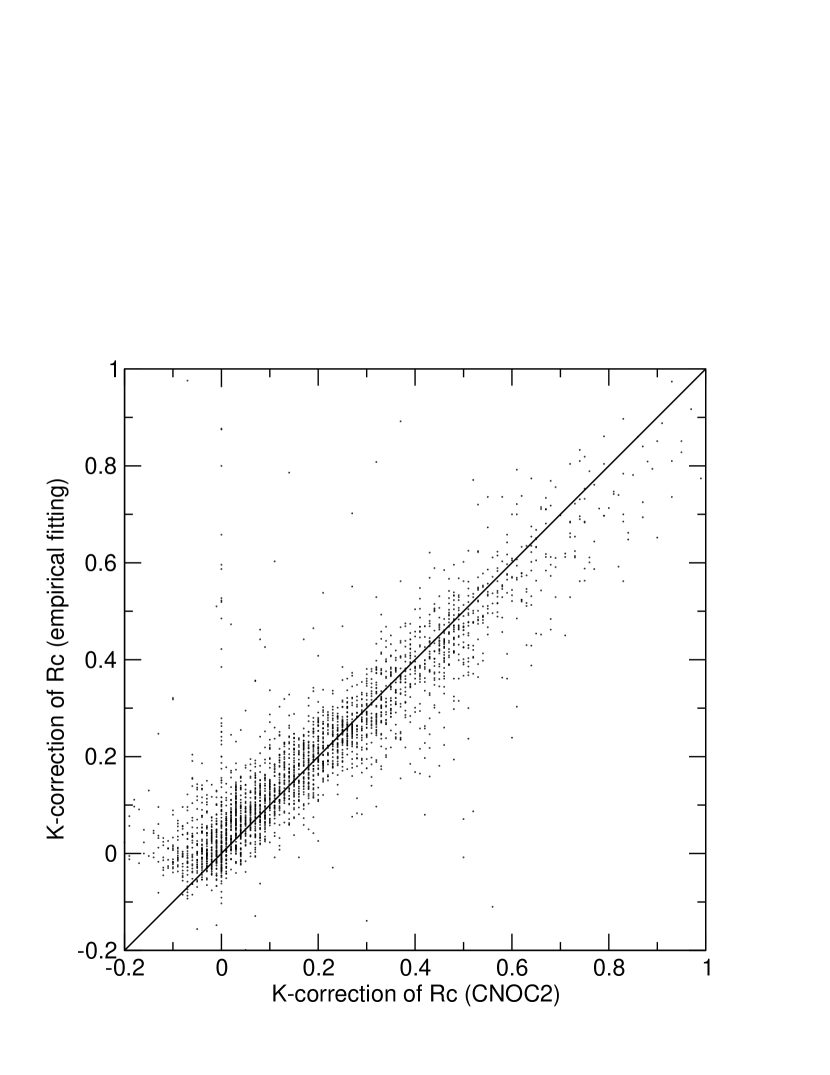
Figure 1: The comparison between the empirical computed K-correction and the K-correction from the CNOC2 catalog. The rms scatter value is about 0.03 mag.

We adopt $Q=1.0$ for the luminosity evolution according to Lin et al. (1999).

3.2 Completeness

The RCS photometric redshift catalog provides the 68% ($\sim 1\sigma$ if the error distribution is Gaussian) computed photometric redshift error for each object. The photometric redshift uncertainty depends on the errors of the photometry for $z^{\prime},R_{c},V,B,$ and colors. The computed error is estimated using a combination of the bootstrap and Monte-Carlo methods and it has been confirmed empirically to be very reliable. The details are described in Hsieh et al. (2005).

For the sample used in the pair analysis, a photometric redshift error cut has to be defined. A looser error cut will make the sample more complete, but the final result will be noisier because data with larger errors are included. A tighter error cut will make the final result cleaner, but the incompleteness and bias problems will be more severe. For example, the bluer objects tend to have larger photometric redshift error and will be rejected more easily than red objects. If the pair result is color-dependent, the conclusion could be biased. As a compromise, we choose $\sigma_{z}/(1+z)\leq 0.3$ to be the criterion for the photometric redshift error cut for the sample. This criterion can eliminate those objects with catastrophic errors, and at the same time, the incompleteness and bias problems will not be too severe. Furthermore, we deal with the incompleteness and bias problems with completeness correction (see § 5.1 for details) to minimize this selection effect.

The completeness correction factor is estimated using the ratio of the total number of galaxies within a 0.1 mag bin at the $R_{c}$ magnitude of the companion to the number of galaxies in that bin with photometric redshifts satisfying the redshift uncertainty criterion. The incompleteness problem is more severe with fainter magnitudes because of the larger photometry uncertainty. Figure 2 represents an example of $R_{c}$ galaxy count histograms for subsamples of various $\sigma_{z}$ criteria for pointing 0224A1. The curves from top to bottom indicate the results with selecting criteria: all objects, objects with photometric redshift solutions, and those with $\sigma_{z}/(1+z)\leq 0.4$, $\sigma_{z}/(1+z)\leq 0.3$, $\sigma_{z}/(1+z)\leq 0.2$, and $\sigma_{z}/(1+z)\leq 0.1$. It is clear that tighter criteria suffer from worse incompleteness at fainter magnitudes.

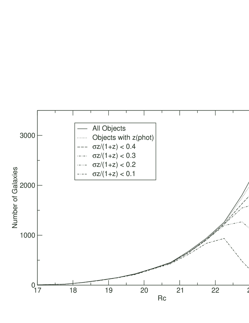
Figure 2: $R_{c}$ histogram for pointing 0224A1 with different sampling criteria. The curves from top to bottom indicate all objects, objects with photometric redshift solutions, and those with $\sigma_{z}/(1+z)\leq 0.4$ to 0.1. It is clear to see that tighter criterion suffers from worse incompleteness.

However, the completeness of the sample depends not only on magnitudes of $z^{\prime},R_{c},V,$ and $B$ but also on colors (e.g., galaxy types). At lower redshift, red objects are more complete than blue objects because early-type (red) galaxies have a clearer 4000Å break which results in better photometric redshift fitting. At higher redshift, the incompleteness for red objects is getting worse (even worse than that of the blue objects) because the photometry of the blue filters is sufficiently deep for blue objects but not for red objects. We refine our completeness correction by computing the factor separately for red and blue galaxies. Figure 3 represents the observed $B-R_{c}$ vs. spectral redshift relation. Most objects in the upper locus are early-type galaxies, and for the lower locus, most of them are late-type galaxies. For the redshift range of our sampling criterion ($0.25\leq z\leq 0.8$), we can simply use $B-R_{c}=1.8$ to roughly separate different types of galaxies.

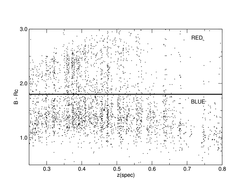
Figure 3: Observed color($B-R_{c}$) vs. spectral redshift from the training set of the RCS photometric redshift catalog (see Hsieh et al., 2005, for details). There are two loci in this plot. Most objects in the upper locus are early-type (red) galaxies, and for the lower locus, most of them are late-type (blue) galaxies. For the redshift range we study ($0.25\leq z\leq 0.8$), a simple constant color cut at $B-R_{c}=1.8$ can roughly separate the different types of galaxies.

3.3 Choosing the Volume Limit

There are two ways to select samples to perform a pair analysis. One is volume-limited selection, the other is flux-limited selection. The volume-limited selection is a proper way to pick up objects with the same characteristics. However, most previous pair studies select flux-limited samples and then try to correct these samples to volume-limited samples using Monte-Carlo simulations (e.g., Patton et al., 2000, 2002; Lin et al., 2004), because of the small number of galaxies in their database. The RCS photometric redshift catalog contains more than one million objects; we can simply select a volume-limited sample and the number of objects is still statistically adequate for pair analysis.

We choose our volume-limited by examining the relationship between the completeness correction factor and absolute magnitude as a function of redshift. Figure 4 shows the average data completeness in the absolute $R_{c}$ magnitude vs. photometric redshift diagrams, with a $\sigma_{z}/(1+z)\leq 0.3$ cut. The upper panel is for patch 0926 and the lower panel is for patch 1327. The contours indicate the completeness correction factors of 1, 2, 3, and 4. According to Figure 4, patch 0926 has much better completeness than patch 1327 in both the absolute $R_{c}$ magnitude axis and the photometric redshift axis.

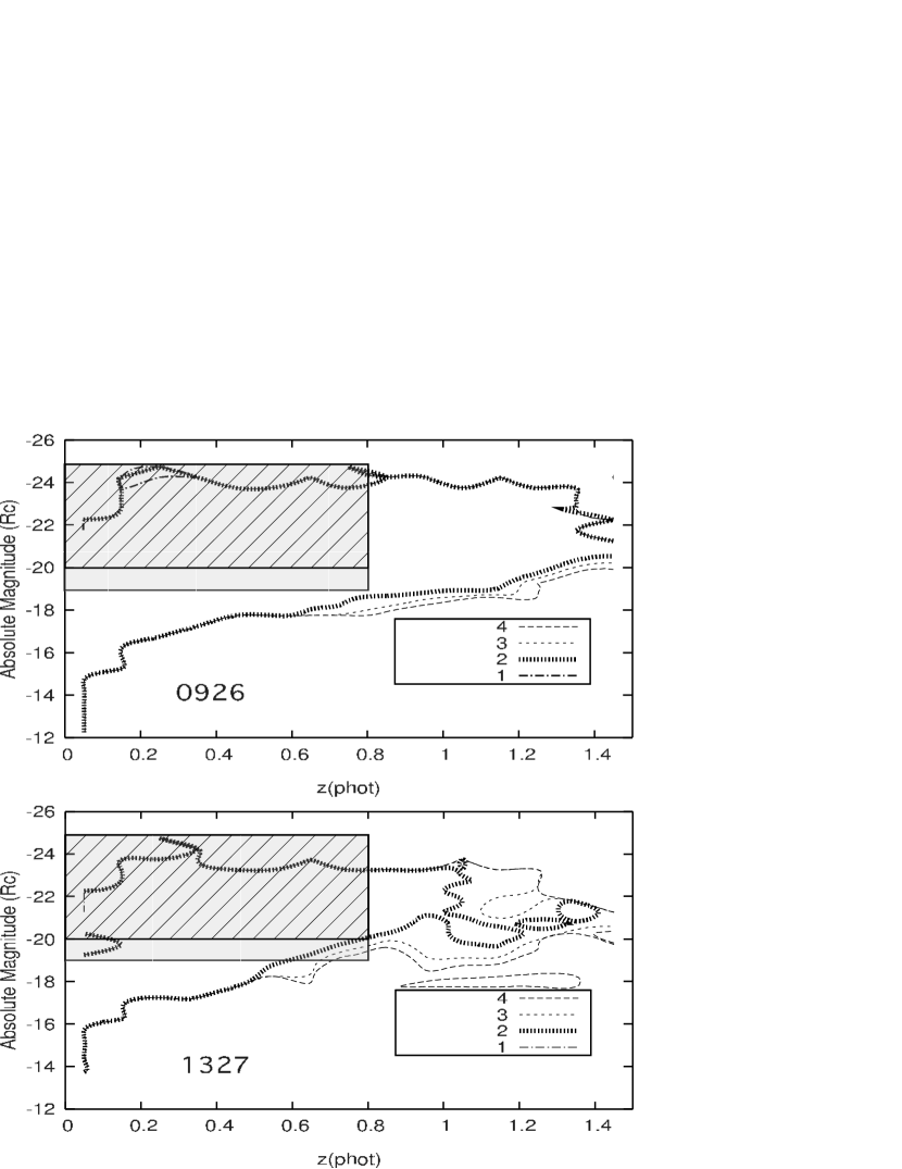
Figure 4: Average data completeness in the absolute $R_{c}$ magnitude vs. photometric redshift diagrams. The upper panel is for patch 0926 and the lower panel is for patch 1327. The contours indicate the completeness correction factors of 1, 2, 3, and 4. According to these two panels, patch 0926 has much better completeness than patch 1327 in both the absolute $R_{c}$ magnitude axis and the photometric redshift axis. We mark our limiting correction factor used to select our sample by the heavy hashed lines. The hatched region shows the selection area of our primary sample; whereas the light shaded area, the secondary sample (see §5.2 for details).

Figure 4 allows us to set reasonable ranges in both the absolute $R_{c}$ magnitude axis and photometric redshift axis for a volume-limited sample. We decide to include data with completeness correction factors less than 2 in our sample, i.e., all the data in our volume-limited sample are at least 50% complete (marked by the heavy hashed lines). While the sample is not 100% complete, the completeness problem can be dealt with the completeness correction later. (See §5.1 for details.) Hence, based on Figure 4 and the diagrams for the other patches, we choose a volume-limited sample using the following criteria: $0.25\leq z\leq 0.8$, $-25\leq M_{R_{c}}\leq-20$ (hatched region), for which the completeness factor is less than 2. We note that at $z=0.8$, and $M_{R_{c}}=-20$, early type galaxy has an $R_{c}\sim 24.7$.

3.4 Choosing Field Galaxies

The pair statistics could be very different in different environments. It is very interesting to study how the environment affects the pair result. However, for a cluster environment, the pair analysis is much more difficult and a significant amount of calibration/correction needs to be done because the pair signals could be embedded in a cluster environment and are difficult to delineate. We may need to develop a different technique for the pair analysis for the highest density regions (i.e., clusters). In this paper, we focus on the pair statistics in the field. The RCS cluster catalogs (Gladders & Yee, 2005) are used to separate the field and the cluster regions. The cluster catalogs provide the information of the red-sequence photometric redshift, astrometry, and $r_{200}$, estimated using the richness $B_{gc}$ statistics of Yee & Ellingson (2003) in Mpc and in arcmin. An object inside $3\times r_{200}$ of a cluster and having a photometric redshift within $z_{cluster}\pm 0.05$ is considered as a potential cluster member. Our rejection of clusters is fairly conservative; we throw away pretty large regions in order to avoid biasing the field estimate, at the expense of having a smaller field sample. Approximately 33% of the galaxies are rejected due to possibly being in clusters. The remaining objects are considered to be in the field and included in our sample.

4 Pair Fraction Measurement

We use the quantity $N_{c}$, defined as the number of close companions per galaxy, which is directly related to the galaxy merger rate, for our pair study. The definition of a close companion is a galaxy within a certain projected separation and velocity/redshift difference ($\Delta{z}$) of a primary galaxy. After counting the number of close companions for each primary galaxy, we calculate the average number of close companions, which is $N_{c}$ (all the projected separations in this paper are in physical sizes, unless noted otherwise).

Previous pair studies with spectroscopic redshift data (e.g., Patton et al., 2000, 2002; Lin et al., 2004) use pair definitions of 5-20 kpc to 5-100 kpc for projected separation, and a velocity difference $<$ 500km/s between the primary galaxy and its companions. However, because of the much larger redshift errors of the photometric redshift data, we cannot use the same criterion of $\Delta{v}$ as other spectroscopic pair studies for our analysis ($\sigma_{z}=0.05$ at $z=0.5$ is equivalent to $\Delta{v}\sim 10000$km/s). Thus, to carry out the pair analysis using a photometric redshift catalog, we develop a new procedure which includes new pair criteria and several necessary corrections.

For the projected separation, we can use the same definition as the spectroscopic pair studies. For the redshift criterion, we utilize the photometric redshift error ($\sigma_{z}$) provided by the RCS photometric redshift catalog to develop a proper definition. We define the redshift criterion of a pair as $\Delta{z}\leq n\sigma_{z}$, where $\Delta{z}$ is the redshift difference between the primary galaxies and its companion, $n$ is a factor to be chosen, and $\sigma_{z}$ is the photometric redshift error of the primary galaxy. Due to the fact that the behavior of the pair fraction for major mergers (pairs with similar mass) and minor mergers (pairs with a huge difference of mass) could be different, one has to give a mass (luminosity) ratio limitation between the primary galaxy and its companion to specify the kind of merger being studied, i.e., $\Delta{R_{c}}\leq x$ mag. We note that the absolute magnitude of $R_{c}$ should be used for the luminosity/mass difference criterion. However, since we use a photometric redshift catalog to perform the pair analysis, the redshifts of the primary and the secondary galaxies may be different due to the photometric redshift errors, which would make the difference of the $k$-corrected absolute magnitudes of the primary and the secondary galaxies larger than the luminosity difference criterion, even if they actually fit the criterion. Hence, we choose to use the apparent magnitude instead of the absolute magnitude.

The quantity $N_{c}$ approximately equals to the pair fraction when there are few triplets or higher order $N$-tuples in the sample. In this study, $N_{c}$ will sometimes simply be referred to as the pair fraction.

5 Accounting for Selection Effects

In this section, we discuss the effects of incompleteness, boundary, seeing and projection, and the steps we take to account for them. In all our subsequent discussions and analyses, we will use samples chosen with the following fiducial common criteria, unless noted otherwise: $-25\leq M_{R_{c}}\leq-20$ for the primary sample, $-26\leq M_{R_{c}}\leq-19$ for the secondary sample, with galaxies selected satisfying $\sigma_{z}/(1+z)<0.3$ and $0.25\leq z\leq 0.8$, and with the pair selection criteria of $\Delta{z}\leq 2.5\sigma_{z}$, 5 kpc $\leq d_{sep}\leq$ 20 kpc, and $\Delta{R_{c}}\leq$ 1 mag.

5.1 Completeness of the Volume-Limited Sample

For a pair analysis, the completeness of the sample is always an important issue. The pair fraction will drop due to the lower number density if the sample is not complete. Furthermore, the main point of this paper is to study the evolution of the pair fraction, and unfortunately, the incompleteness is not independent of redshift: it gets more serious at higher redshifts. This effect is expected to make the pair fraction at higher redshifts appear lower, and thus may bias conclusions regarding the redshift evolution of the pair fraction. Hence, to draw the correct conclusion, a completeness correction has to be applied.

Figure 5 illustrates the pair fractions for different sampling criteria in $\sigma_{z}/(1+z)$ without completeness corrections (but with projection correction, see §5.3). Each redshift bin contains from 15,500 objects (for the $\sigma_{z}/(1+z)\leq 0.1$ criterion) The plot shows that the larger the $\sigma_{z}$ criterion, the higher the pair fraction. This is due to less completeness for a tighter criterion; some real companions in pairs are missed because they have larger photometric redshift errors. The differences between the pair fractions with different $\sigma_{z}/(1+z)$ criteria also become larger with redshift because the incompleteness is more severe at higher redshift, especially for the $\sigma_{z}/(1+z)\leq 0.1$ criterion. However, if a proper completeness correction is adopted, the pair results should not be affected by the sampling criteria and these curves of pair fraction with different $\sigma_{z}/(1+z)$ cuts should be similar.

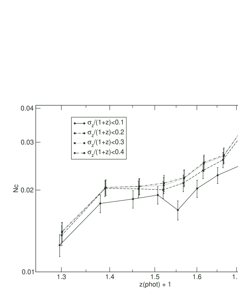
Figure 5: Pair fractions with different $\sigma_{z}/(1+z)$ of the sampling criteria without the completeness correction (but with the projection correction). Each redshift bin contains from 15,500 objects (for the $\sigma_{z}/(1+z)\leq 0.1$ criterion) to 17,500 objects (for the $\sigma_{z}/(1+z)\leq 0.4$ criterion). Note that the larger the $\sigma_{z}/(1+z)$, the higher the pair fraction, which is due to the lower completeness for samples with a tighter redshift uncertainty criterion, causing some companions to be missed in the pair counting.

We discussed the derivation of the completeness correction in §3.2, and after applying the completeness correction, we find the pair fractions to be very similar for the different redshift uncertainty criteria, which shows that the completeness correction works well. The results after the completeness correction are shown in §7.

5.2 Boundary Effects

Objects near the boundaries of the selection criteria or close to the edges of the observed field could have fewer companions. This effect is referred to as a boundary effect. There are four different boundaries for our sample: $1)$ the boundaries of the selection criterion on the redshift axis; $2)$ the edge of the observing field; $3)$ the boundaries between the cluster region and the field; and $4)$ the boundary of the absolute magnitude $M_{R_{c}}$ cut. The methods to deal with these boundary effects are described in this subsection.

The redshift range for our pair analysis is $0.25\leq z\leq 0.8$. For primary galaxies at redshift close to 0.25 or 0.8, they will have fewer companions because some of their companions are scattered just outside the redshift boundaries and thus are not counted. To deal with this effect, we conduct the pair analysis for the full redshift range of the photometric redshift catalog ($0.0<z<1.5$), and then pick the primary objects satisfying the redshift criteria for the final result.

The objects near the boundaries of the observing field or near the gaps between CCD chips will have smaller pair fractions because some companions of these objects lie just across the boundaries of the observing field. The projected size of 20 kpc (the outer radius of pair searching circle) is about 5” (24 pixels) at redshift at 0.25; the size gets smaller at higher redshift. We limit the primary sample to be at least 5” from the edges of the CCDs while the secondary sample still includes all the objects. This configuration allows us to avoid the boundary effect of the limited survey fields.

Because we only study the pair fraction in the field for this investigation and separate our data into field environment and cluster environment, the boundary effect at the edges of $3\times r_{200}$ and $z_{cluster}\pm 0.05$ is of concern. We constrain the primary sample to be at least $3\times r_{200}$ from the centers of clusters and $\Delta{z}>0.1$ from $z_{cluster}$. For the secondary sample, we limit it to be at least $3\times r_{200}-10"$ from the center of clusters and $\Delta{z}>0.05$ from $z_{cluster}$. These new limits effectively eliminate these boundary effects.

The objects with absolute magnitudes close to the $M_{R_{c}}$ cut will have a lower pair fraction as well. This can be solved easily by searching for companions down to $M_{R_{c}}\leq-19$ for the primary sample with $M_{R_{c}}\leq-20$. Figure 4 shows that the completeness correction factors are still less than 2 even when we push the $M_{R_{c}}$ boundary to -19 at $z\leq 0.8$ for patch 0926 (the light shaded area). However, for patches 0351 and 1327, the completeness is significantly worse than other 8 patches, and they are substantially incomplete at $M_{R_{c}}=-19$. Hence, they are abandoned in our pair analysis. Consequently, the magnitude limit for the secondary sample is extended to minimize this boundary effect.

5.3 Projection Correction

Because of the projection effect due to the lower accuracy of the photometric redshifts compared with spectroscopic redshifts, a pair analysis using any criterion would find some false companions and get a higher $N_{c}$ than the real value. To eliminate these foreground and background objects from contaminating our results, a projection correction is applied to our data.

The magnitude of the projection effect on $N_{c}$ is illustrated in Figure 6 which shows the results of using the fiducial sample but with different $z_{primary}\pm n\sigma_{z}$ criteria for inclusion of the companion without any projection correction (but with completeness correction). Each data point contains about 17,500 objects. $N_{c}$ is higher with larger $n$ values because the pair criterion with larger $n$ includes more foreground/background galaxies and the results suffer from more serious projection effect. For lower redshift, the projected search area is bigger than the one for higher redshift; hence more foreground/background galaxies are counted. However, the photometric redshift error $\sigma_{z}$ becomes larger at higher redshift; this effect also makes more foreground/background galaxies included. Therefore, from low redshift to high redshift, the projection effect affects the pair fraction about equally.

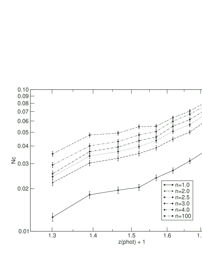
Figure 6: Pair fractions with different $z_{primary}\pm n\sigma_{z}$ criteria without any projection correction (but with completeness correction). Each data point contains about 17,500 objects. The pair fraction increases with larger $n$ value because the pair criterion with larger $n$ includes more foreground/background galaxies and the results suffer from more serious projection effect. Note that the $n=100$ curve is approximately equivalent to not having photometric information.

To correct for the projection effect, we calculate the mean surface density of all the objects in the same patch as the primary galaxy satisfying the pair criteria, $\Delta{z}\leq n\sigma_{z}$ and $\Delta{R_{c}}\leq 1$ mag, and then multiply it by the pair searching area (5-20 kpc) for each primary galaxy. This is the projection correction value for each primary galaxy. The completeness corrections are also applied in the counting of the foreground/background galaxies. The final number of companions for each galaxy is the proper companion number with the projection correction value subtracted. Because not all primary objects have companions, some objects have negative companion numbers after the projection correction.

5.4 The Effect of Seeing

The projected separation we use for the pair criteria is 5 kpc $\leq d_{sep}\leq$ 20 kpc. For the highest redshift cut ($z=0.8$) used in our analysis, the projected size is about three pixels (0”.7) for 5 kpc (the inner radius). However, some data are taken in less favorable weather conditions, and the 5 kpc inner radius could be too small for these data due to poor resolution. In the meantime, we do not want to enlarge the inner radius because the closest pairs are the most important for a pair study. We have to make sure that the 5 kpc inner searching radius does not cause problems with data obtained in poorer seeing conditions.

We only focus on the seeing conditions of the $R_{c}$ images because object finding was carried out using the $R_{c}$ images (see Hsieh et al. 2005 for details). The distribution of the seeing conditions of $R_{c}$ for the 8 patches is shown in Figure 7. From this plot, most seeing values are between three to six pixels. To test if the inner radius (5 kpc) of the searching criterion is too small for data taken in poorer seeing conditions, we perform the pair analyses for three subsamples with different seeing conditions separately, separated at seeing $=3.81$ pixels (0$"$.78) and $4.70$ pixels (0$"$.97). Each subsample contains a similar number of pointings. The results are shown in Figure 8. The left panel represents the relation of the apparent size in pixels for different physical sizes (5, 10, 15, and 20 kpc) vs. redshift, as a reference, while the right panel shows the results with different seeing conditions. There are about 10,000 objects in each redshift bin. We find that the curve with the best seeing condition is in fact about 20% lower than the other two poorer seeing conditions, indicating that the range of seeing in our data do not cause a drop in $N_{c}$. We note that most pointings with the best seeing conditions are from patches 1416 and 1616; the 20% lower $N_{c}$ for the good seeing data could be just due to cosmic variance. Therefore, the 5 kpc inner searching radius for all the data does not appear to produce a significant selection effect on the result.

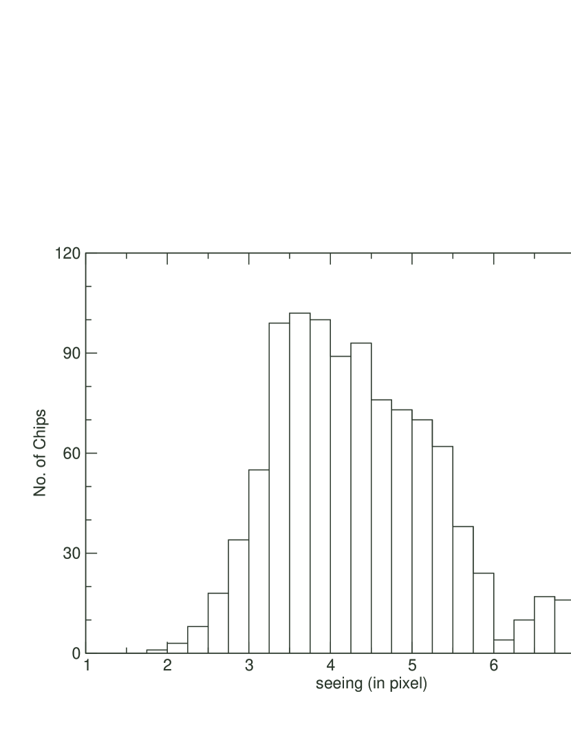
Figure 7: Histogram of seeing condition for the $R_{c}$ images. Most of the seeing values are about four pixels ($\sim 0".82$), but there are still some images taken under very poor weather with seeing up to 8 pixels.

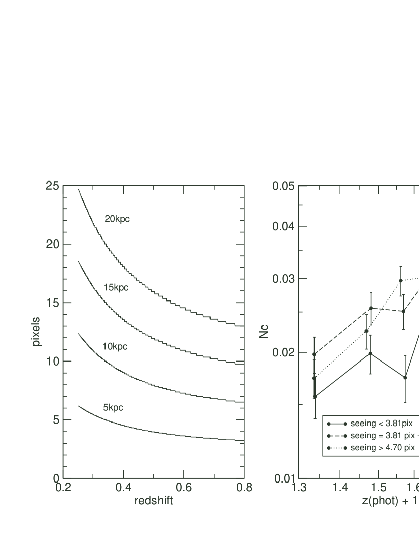
Figure 8: Pair fractions of the data taken under different seeing conditions. The left panel represents the relation of the apparent size in pixels for different physical sizes (5, 10, 15, and 20 kpc) vs. redshift, as a reference, while the right panel shows the results with different seeing conditions. The curves in the right panel indicate the pair fraction of data taken under different weather conditions. There are about 10,000 objects in each redshift bin. We find that the curve with the best seeing condition is in fact about 20% lower than the other two worse seeing conditions, indicating that the range of seeing in our data do not cause a drop in $N_{c}$. We note that most pointings with the best seeing condition are from two patches; the somewhat lower $N_{c}$ for the good seeing data could be just due to cosmic variance.

6 Error Estimation of $N_{c}$

The error of $N_{c}$ is estimated assuming Poisson distribution and derived using:

$$error=\frac{\sqrt{N_{companion}+N_{proj}}}{N_{primary}}$$ (2)

where $N_{companion}$ is the total number of the companions, $N_{proj}$ is the sum of the projection correction values, and $N_{primary}$ is the number of the primary galaxies in each redshift bin. We note that the values of $N_{companion}$ and $N_{proj}$ are the ones without the completeness corrections in order to retain the correct Poisson statistics.

7 Results

The results of the pair analysis are shown in Figures 9 to 13. Because we focus only on major mergers, the difference in $R_{c}$ between the galaxies in close pairs is restricted to be less than one magnitude. If the mass-to-light ratio is assumed to be constant for different types of galaxies at the same redshift, the mass ratio between the primary galaxies and companions ranges from 1:1 to 3:1.

Figure 9 shows the results with different $\sigma_{z}/(1+z)$ cuts, with the fiducial sampling criteria listed in §5, with completeness and projection corrections applied. The redshift bins contain from 15,500 objects (for the $\sigma_{z}/(1+z)\leq 0.1$ criterion) to 17,500 objects (for the $\sigma_{z}/(1+z)\leq 0.4$ criterion). Compared to Figure 5, the curves of the pair fractions are very similar for the different redshift uncertainty criteria, which illustrates that the completeness correction works well.

For the redshift criterion of the pair definition, we count companions within $z_{primary}\pm n\sigma_{z}$, where $z_{primary}$ is the redshift of the primary galaxy and $\Delta{z}=n\sigma_{z}$ (see §4). If the photometric redshift error is assumed to be Gaussian, when $n=1.0$, we count only about 68% of the companions; when $n=2.0$, about 95%; and so on. Of course, the criteria with larger $n$ will include more foreground/background galaxies and make $N_{c}$ higher, but this can be dealt with by the projection correction (see § 5.3 for details).

Figure 10 represents $N_{c}$ vs. photometric redshift curves using different $\Delta{z}=n\sigma_{z}$ criteria with the fiducial sampling criteria, with completeness and projection corrections applied. Pair fractions using the values $n=1.0,2.0,2.5,3.0,4.0,$ and $100.0$ are plotted. We use $n=100.0$ to approximate $n=\infty$ which is equivalent to the result using no redshift information for companions. Each data point contains about 17,500 objects. Curves with $n\geq 2.5$ are consistent with being the same. As discussed, the curve with $n=1.0$ should be about 32% lower than the one with $n=100.0$ if the distribution of the photometric redshift error is Gaussian. The curve with $n=1.0$ is about 40% lower than the one with $n=100.0$, and about 30% lower than the one with $n=2.5$. While the results do not perfectly match what is expected from a Gaussian distribution of photometric redshift uncertainties, comparing Figure 10 to Figure 6, the application of the projection correction does reduce the $N_{c}$ derived by approximately the correct amount. The somewhat larger difference is not unexpected, since the true probability distribution of the uncertainty of the photometric redshift is likely non-Gaussian, but somewhat broader. We note that the error bars with larger $n$ are bigger because of larger projection correction errors (see §6 for details). We choose $n=2.5$ for our final result; with this, about 99% of the companions are counted, which is a compromise between the completeness of the companion counting and the size of the error of the projection correction.

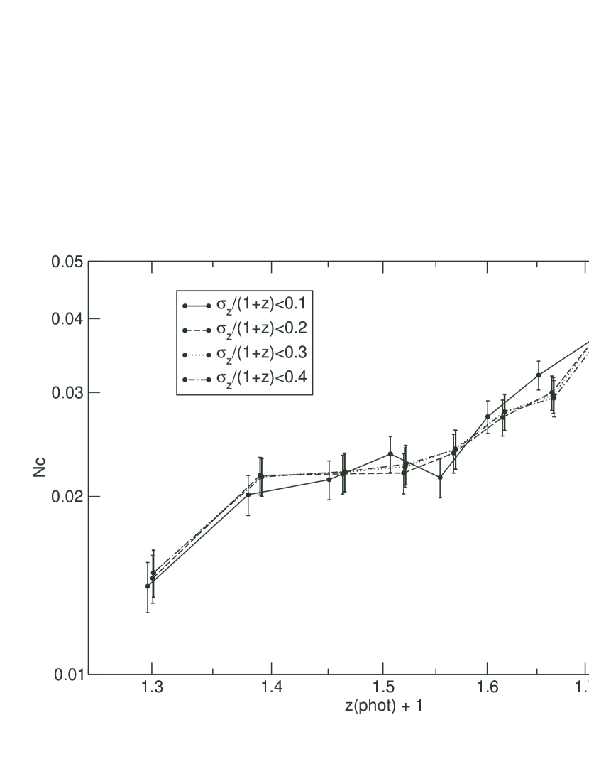
Figure 9: Pair fraction vs. redshift after the completeness correction, with different redshift uncertainty (in $\sigma_{z}/(1+z)$) criteria, using the the sampling criteria: $-25\leq M_{R_{c}}\leq-20$ for the primary sample, $-26\leq M_{R_{c}}\leq-19$ for the secondary sample, $0.25\leq z\leq 0.8$, and the pair criteria: 5 kpc $\leq d_{sep}\leq$ 20 kpc, $\Delta{z}\leq 2.5\sigma_{z}$, $\Delta{R_{c}}\leq 1$ mag. The completeness and projection corrections are applied. Each redshift bin contains from 15,500 objects (for the $\sigma_{z}/(1+z)\leq 0.1$ criterion) to 17,500 objects (for the $\sigma_{z}/(1+z)\leq 0.4$ criterion). Comparing to Figure 5, the curves of pair fractions are very similar for the different redshift uncertainty criteria, which shows that the completeness correction works well.

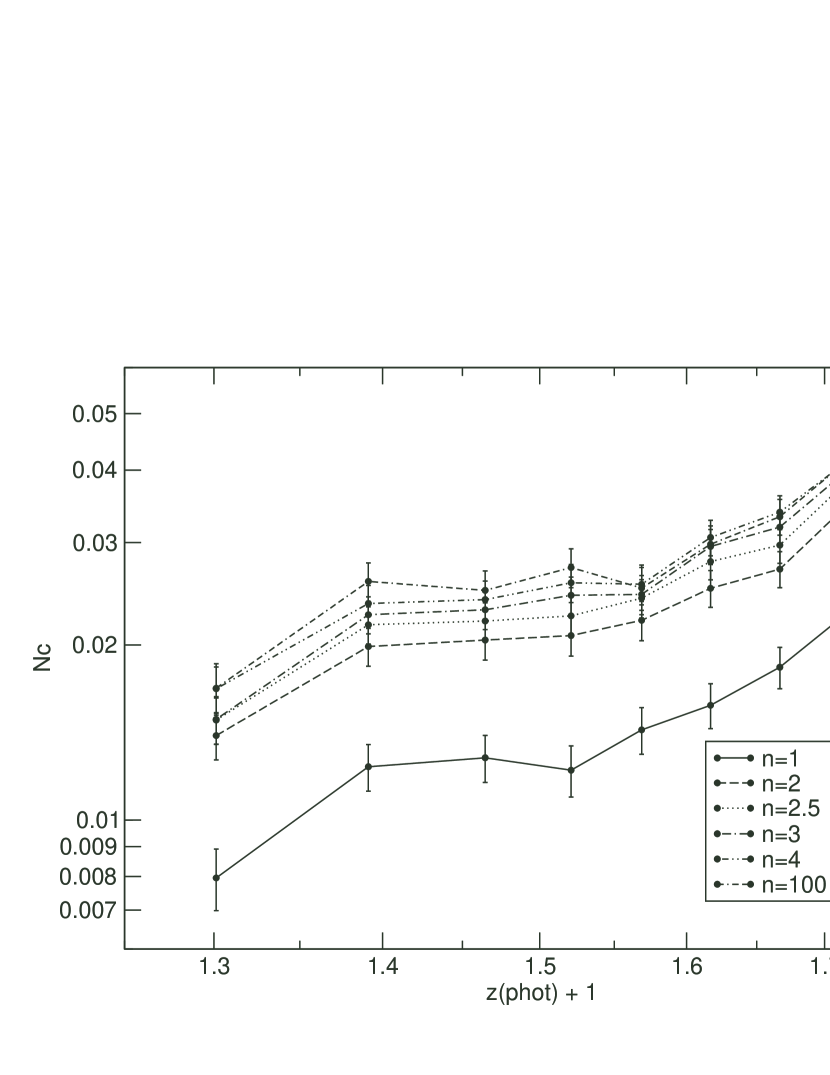
Figure 10: Pair fraction vs. photometric redshift curves with different $\Delta{z}=n\sigma_{z}$ criteria. The projected separation criterion used in this plot is 5-20 kpc. The completeness and projection corrections are applied. Pair fractions using the parameter $n=1.0,2.0,2.5,3.0,4.0,$and $100.0$ are plotted. We use $n=100.0$ to approximate $n=\infty$ which indicates the result using no redshift information for companions. Each data point contains 17,500 objects. Note that curves with $n\leq 2.5$ are consistent with being the same. The curve with $n=1.0$ is expected to be about 32% lower than the one with $n=100.0$ if the distribution of the photometric redshift error is Gaussian. The $n=1.0$ result is about 40% and 30% lower than the ones with $n=100.0$, and $n=2.5$, respectively.

In Figure 11, we show $N_{c}$ using different outer radii of the projected separations for the pair criterion. The completeness and projection corrections are applied. We use an inner radius of 5 kpc for all cases. Different line types and symbols indicate different outer radii from 20 kpc to 100 kpc. As expected, the larger the outer radius, the higher the $N_{c}$ because more galaxies satisfy the pair criteria. For better statistics, and because most previous pair studies use 5-20 kpc as their pair criteria (since pairs with separations of 20 kpc will be almost certain to merge), we choose 5 kpc $\leq d_{sep}\leq$ 20 kpc to be the pair criterion for the projected separation for this study.

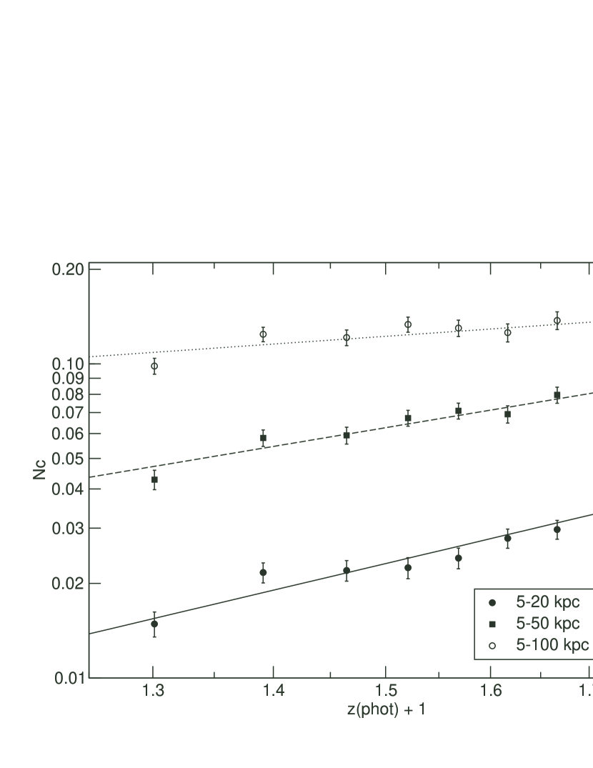
Figure 11: Pair fractions using different projected separations for the pair criterion. There are about 17,500 objects in each redshift bin. The completeness and projection corrections are applied. The inner radius is 5 kpc. Different line types and symbols indicate different outer radii from 20 kpc to 100 kpc. Generally speaking, the larger the outer radius, the higher the pair fraction because more galaxies satisfy the pair criteria.

Using 5 kpc $\leq d_{sep}\leq$ 20 kpc and $\Delta{z}\leq 2.5\sigma_{z}$, as our fiducial criteria, we find that the pair fraction increases with redshift as $(1+z)^{m}$ where $m=2.83\pm 0.33$. The best fit is plotted as a solid line on Figure 11. The error is estimated using the Jackknife technique. We note that the error bar of the $m$ value is affected not only by the error bar of each redshift bin but also by whether the function $(1+z)^{m}$ is a good representation of the data.

We also study the pair fractions with different absolute magnitude $M_{R_{c}}$ cuts and show the results in Figure 12. The filled circles and the open squares indicate the absolute magnitude bins of $-21\leq M_{R_{c}}\leq-20$ and $-25\leq M_{R_{c}}<-21$, respectively. The numbers of objects in each redshift bin with absolute magnitude cuts for faint and bright are about 15,700 and 10,500, respectively. We find that the pair fraction increases with redshift as $(1+z)^{m}$ where $m=3.25\pm 0.11$ (solid line) and $m=1.79\pm 0.53$ (dashed line) for the absolute magnitude bins of $-21\leq M_{R_{c}}\leq-20$ and $-25\leq M_{R_{c}}<-21$, respectively; i.e., the brighter the absolute magnitude, the smaller the $m$ value. However, the error bar of the $m$ value is significantly larger for the high-luminosity sample. This effect is not due to the slightly larger error bars in the bright sample, but rather that the $(1+z)^{m}$ power-law does not appear to be a good representation of the evolution of $N_{c}$ for the higher luminosity galaxies. This result is further discussed in §8.

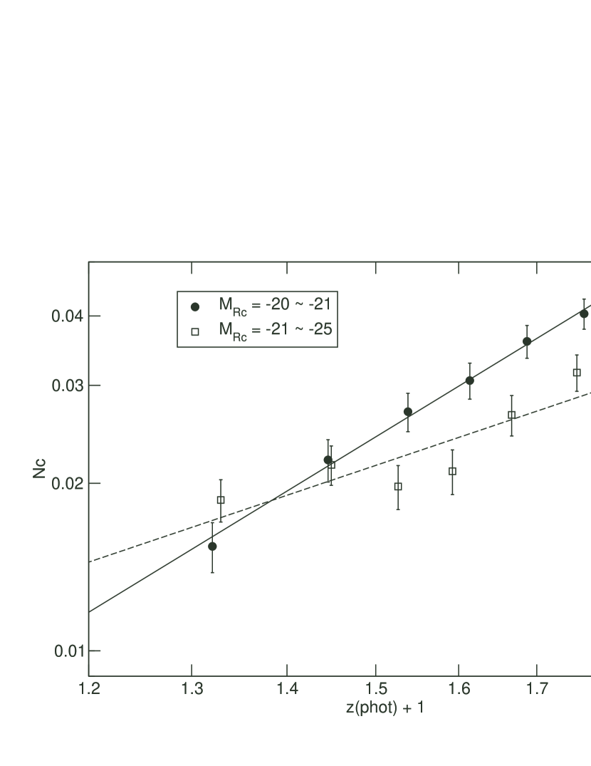
Figure 12: Pair fractions with different $M_{R_{c}}$ bins. The filled circles and the open squares indicate the absolute magnitude bins of $-21\leq M_{R_{c}}\leq-20$ and $-25\leq M_{R_{c}}<-21$, respectively. The numbers of objects in each redshift bin with absolute magnitude cuts for faint and bright are 15,700 and 10,500, respectively. We find that the pair fraction increases with redshift as $(1+z)^{m}$ where $m=3.25\pm 0.11$ (solid line) and $m=1.79\pm 0.53$ (dashed line) for the absolute magnitude bins of $-21\leq M_{R_{c}}\leq-20$ and $-25\leq M_{R_{c}}<-21$, respectively, i.e., the brighter the absolute magnitude, the smaller the $m$ value.

Based on Figure 11, it is apparent that the larger the outer radii, the lower the $m$ value is. To look at this in more detail, we use rings of area for the pair counting, and show the results of the evolution of $N_{c}$ in Figure 13. We note that all $N_{c}$ values are normalized by area using the 5-20 kpc bin as the reference. The number of objects in each redshift bin is about 17,500. The evolution of the pair fraction follow $(1+z)^{m}$ where $m=2.83\pm 0.33,1.53\pm 0.36,-0.39\pm 0.36$, and $-1.20\pm 0.48$ for separation 5-20 kpc, 20-50 kpc, 50-100 kpc, 100-150 kpc, respectively. We note that the $m$ value decreases with increasing separation. This result is further discussed in §8.

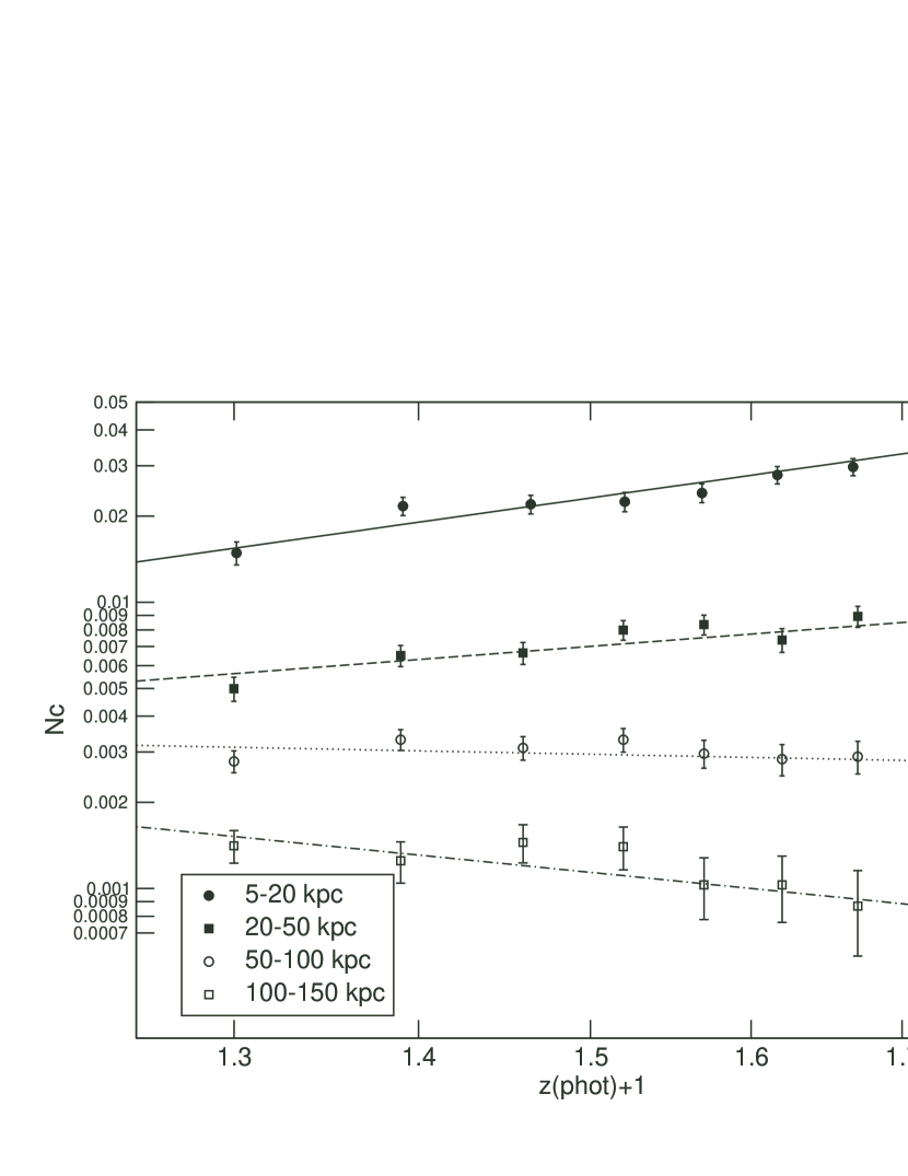
Figure 13: Pair fractions with different projected pair separation bins. The number of objects in each redshift bin is about 17,500. The evolutions of the pair fraction follow $(1+z)^{m}$ where $m=2.83\pm 0.33,1.53\pm 0.36,-0.39\pm 0.36$, and $-1.20\pm 0.48$ for separation 5-20 kpc, 20-50 kpc, 50-100 kpc, and 100-150 kpc, respectively. We note that the $m$ value decreases with increasing separation.

All these results show that the pair fractions do not change much with different $\Delta{z}=n\sigma_{z}$ criteria after applying the completeness and projection corrections, which indicates that our results are very robust; however, the results do change with different projected separation criteria and absolute magnitude cuts.

We note that the role of photometric redshift in reducing the size of the projection effect is relatively limited, as indicated by the similar error bars for the pair fractions in Figure 6 for different $n$. This is because the criterion of $\Delta m=\pm 1$ effective eliminates most of the foreground background galaxies. However, photometric redshift is essential in defining a volume-limited sample and deriving the redshift dependence of $N_{c}$.

8 Discussions

8.1 Major Merger Fraction

Although we have applied projection correction for our pair analysis, not all the close pairs we count will result in real mergers. Objects satisfying the pair criteria that are in the same structure (i.e., under each other’s gravitational influence) are within 20 kpc projected distance, but not within 20 kpc in real 3-D space distance. Yee & Ellingson (1995) estimates that the true merger fraction ($f_{mg}$) is about half of the pair fraction which is evaluated with a triple integral over projected and velocity separation by placing the correlation function into redshift space. Hence, we divide $N_{c}$ by 2 to calculate the merger fraction.

8.1.1 Merger Timescale

Close pairs are considered as early-stage mergers. To relate the close pairs to the overall importance of merger, the merger timescale ($T_{mg}$) has to be estimated. Following previous studies (Binney & Tremaine, 1987; Patton et al., 2000), assuming circular orbits and a dark matter density profile given by $\rho(r)\propto r^{-2}$, the dynamical friction timescale ($T_{mg}$ in Gyr) is given by:

$$T_{mg}=\frac{2.64\times 10^{5}r^{2}v_{c}}{M\ln\Lambda},$$ (3)

where $r$ is the physical pair separation in kpc, $v_{c}$ is the circular velocity in km s^-1, $M$ is the mass in $M_{\odot}$, and ln $\Lambda$ is the Coulomb logarithm. We adopt the average projected separation ($\sim$ 15 kpc) as the physical pair separation since the major merger fraction has been corrected from projected separation to three-dimensional separation. We also assume $v_{c}\sim 250$ km s^-1. The mean absolute magnitude of companions is $M_{R_{c}}\sim-20.5$. If the mass-to-light ratio of $M/L\sim 5$ is assumed, we derive a mean mass of $M\sim 5\times 10^{10}M_{\odot}$. Dubinski, Mihos, & Hernquist (1999) estimates ln $\Lambda\sim 2$. With these values, we find $T_{mg}\sim 0.5$ Gyr. We note that this value is just a rough estimate over systems with a wide range of merger timescales, but it still represents the average merger timescale in our sample.

8.1.2 Merger Rate

The comoving merger rate is defined as the number of mergers per unit time per unit comoving volume. According to Lin et al. (2004), it can be estimated as:

$$N_{mg}=0.5n(z)N_{c}(z)C_{mg}T_{mg}^{-1},$$ (4)

where $T_{mg}$ is the dynamical friction timescale, $C_{mg}$ indicates the fraction of galaxies in close pairs that will merge in $T_{mg}$, and $n(z)$ is the comoving number density of galaxies. The factor 0.5 is to convert the number of galaxies into the number of merger events. We adopt $T_{mg}=0.5$ Gyr and $C_{mg}=0.5$, as discussed above. We compute $n(z)$ using the primary sample, with the weight corrections included. We note that the computed $n(z)$ show a slight decline at $z>0.5$, which may be an indication of the effect of using a simple luminosity evolution description of $Qz$ for $M^{*}$ for choosing the sample. The evolution of the merger rate is shown in Figure 14. Each data point includes 17,500 objects and the error bars do not include the uncertainties in $T_{mg}$ and $C_{mg}$. Comparing our merger rate to Lin et al. (2004) measured between $z\sim 0.5$ to 1.2, our value is about 3 times lower. The primary reason is likely that we use $\Delta{R_{c}}\leq 1$ mag and search for major mergers with mass ratio from 1:1 to 3:1, but Lin et al. (2004) look for mergers with mass ratio from 1:1 to 6:1. Our results show an increase in the merger rate with redshift of the form $(1+z)^{\beta}$, with $\beta\sim 0.8$.

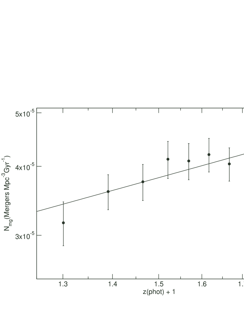
Figure 14: Comoving merger rate vs. photometric redshift. Each data point includes 17,500 objects and the error bars do not include the uncertainties in $T_{mg}$ and $C_{mg}$. The solid line is a fit of the form $(1+z)^{\beta}$, with the slope $\beta\sim 0.8$.

8.1.3 Major Merger Remnant Fraction

With the derived major merger rates for several different epochs for $z<0.8$ and the merger timescale, we can use these parameters to estimate the fraction of present day galaxies which have undergone major mergers in the past. These galaxies are merger remnants, and the fraction of the merger remnants is defined as the remnant fraction ($f_{rem}$). According to Patton et al. (2000), the remnant fraction is given by

$$f_{rem}=1-\prod^{N}_{j=1}\frac{1-f_{mg}(z_{j})}{1-0.5f_{mg}(z_{j})}$$ (5)

where $f_{mg}$ is the merger fraction, $z_{j}$ is the redshift which corresponds to a lookback time of $t=jT_{mg}$, and j is an integer factor. Because the mass ratio of galaxies in a pair for this study is from 1:1 to 3:1, the merger remnant fraction is for major mergers. After applying this equation to our pair result, the estimated remnant fraction is $f_{rem}=0.06$, which implies that $\sim 6\%$ of galaxies with $-25\leq M_{R_{c}}\leq-20$ have undergone a major merger since $z\sim 0.8$.

8.2 Evolution of the Pair Fraction

The $m$ values determined in many previous observational results in similar redshift ranges are very diverse ($0\leq m\leq 4$). These results from the literature are listed in Table 1 in the order of redshift, and briefly discussed in §1. From $\Lambda$ CDM $N$-body simulations (Governato et al., 1999; Gottlöber et al., 2001), the merger rates of halos increases with redshift as $(1+z)^{m}$, with $2.5\leq m\leq 3.5$. Our result for $-25\leq M_{R_{c}}\leq-20$ is broadly consistent with the $N$-body simulations as well as all the previous observational results, except those of Lin et al. (2004) and Bundy et al. (2004). Most of the previous works, except that of Kartaltepe et al. (2007), used spectroscopic redshifts to study pairs, especially for the lower redshift ranges. Due to much smaller samples ( $<1/20$ of our sample) these studies need to convert a flux-limited sample to a volume-limited sample; this conversion may affect the final results. We note that all the previous studies did not exclude possible cluster environments, which may cause a problem of transforming $N_{c}$ to pair fraction, just because a galaxy would have a much higher chance to have more than one companion in cluster environments, relative to in field environments; the value of average number of companions per galaxy is not a good representation of pair fraction anymore. We do not have this problem because potential cluster members in our sample are removed, and less than 2% of pairs actually consists of triples or more in our work.

Table 1: $m$ values from different references

Sample	$m$ value	Redshift Range	Photometry Criteria
This Work	$2.83\pm 0.33$	0.25 $\leq z\leq$ 0.80	-25 $\leq M_{R_{c}}\leq$ -20, field galaxies
Governato et al. (1999); Gottlöber et al. (2001)	$2.5\sim 3.5$		$\Lambda$ CDM $N$-body simulations
Zepf & Koo (1989)	$4.0\pm 2.5$	$z<0.25$	$B\leq 22$
Yee & Ellingson (1995)	$4.0\pm 1.5$	$z<0.38$	$r\leq 21.5$
Carlberg, Pritchet & Infante (1994)	$3.4\pm 1.0$	$z<0.4$	$V\leq 22.5$
Patton et al. (1997)	$2.8\pm 0.9$	$z\leq 0.45$	$r\leq 22$
Patton et al. (2002)	$2.3\pm 0.7$	0.12 $\leq z\leq$ 0.55	$R_{c}\leq 21.5$, Q=1
Burkey et al. (1994)	$3.5\pm 0.5$	$z<0.7$	$I\leq 22.3$
Le Févre et al. (2000)	$2.7\pm 0.6$	$z<1$	$I_{AB}\leq 22.5$ for primary, $I_{AB}\leq 24.5$ for secondary
Lin et al. (2004)	$1.60\pm 0.29$	$0.45<z<1.2$	$R_{AB}\leq 24.1$
Lin et al. (2004)	$0.51\pm 0.28$		Q=1
Kartaltepe et al. (2007)	$3.1\pm 0.1$	$0<z<1.2$	$M_{V}<-19.8$, photometric redshift
Kartaltepe et al. (2007)	$2.2\pm 0.1$		Q=1
Bridge et al. (2007)	$2.12\pm 0.93$	$0.2<z<1.3$	$L_{IR}\leq 10^{11}L_{\odot}$
Bundy et al. (2004)	no evolution	$0.5<z<1.5$	$K\leq 22.5$
Cassata et al. (2005)	$2.2\pm 0.3$	$z<2$	$K_{s}<20$

The only previous work using a similar technique (photometric redshifts) with comparable size (59,221 galaxies, about 2.5 times smaller than our sample) is Kartaltepe et al. (2007). They have a higher redshift limit ($z=1.2$) comparing with ours ($z=0.8$), while we have a considerably larger survey field (33.6 deg² vs. 2 deg²). They also have a similar luminosity cut ($M_{V}=-19.8$, equivalent to $M_{R_{c}}\sim-20.3$) to that of our primary sample ($M_{R_{c}}=-20.0$), although we have a one-magnitude deeper luminosity cut for the secondary sample ($M_{R_{c}}=-19.0$) which properly deals with the boundary problem (see §5.2). Since we apply luminosity evolution in our analysis, we compare our result to the $m$ value of Kartaltepe et al. (2007) derived with luminosity evolution. The $m$ value of our study is somewhat higher, $2.83\pm 0.33$ vs. $2.2\pm 0.1$, but within statistical consistency.

We further separate our sample with different luminosities, as shown in Figure 12. In general, the pair fraction for luminous galaxies is lower than that of the fainter sample. The $m$ values are $3.25\pm 0.11$ and $1.79\pm 0.53$ for $-21\leq M_{R_{c}}\leq-20$ and $-25\leq M_{R_{c}}<-21$, respectively. From the result of the $m$ values, it appears that the pair fraction for the faint galaxy sample evolves more rapidly than the luminous galaxy sample. However, we note that the evolution of $N_{c}$ for the bright sample may not fit a single power law very well. The data suggest that $N_{c}$ may level out at $z\lesssim 0.6$, while at $z\gtrsim 0.6$, the $m$ value is similar to that for the faint sample. It is not clear what produces this possible leveling of the evolution for the bright sample. A larger sample of galaxies will be useful in examining the dependence of the pair fraction evolution as a function of luminosity or stellar mass.

We also study the evolution of pair fractions for different projected separations. As shown in Figure 13, the $m$ value decreases with increasing separation; i.e., the evolution gets weaker for larger separation. This suggests that the timescale of a galaxy going from 20 kpc to 0 (i.e., merged), relative to the timescale for galaxies going in at 50 kpc, increases at higher redshift, so that there is a build up of galaxies at 5-20 kpc. Alternatively, this difference in $m$ values may be the steepening of the galaxy - galaxy correlation function at very small scales at higher redshift. Such steepening, at somewhat larger radius, has been observed (Pollo et al., 2006; Coil et al., 2006). The difference of timescale could be due to higher concentration in the galaxy haloes at lower redshift. For a given mass of dark halo, the density is higher in the inner region for a high concentration halo, relative to a low concentration halo; however, the density is lower in the outer region for a high concentration halo. Therefore, for a high concentration halo, the dynamical friction timescale would be longer in the outer region and shorter in the inner region. Hence, our results suggest that for a given mass, the galaxy dark halo size is smaller at lower redshift, which is consistent with the simulation results from Bullock et al. (2001). Bullock et al. studied dark matter halo density profile parameterized by an NFW (Navarro, Frenk, & White, 1997) form in a high-resolution $N$-body simulation of a $\Lambda$CDM cosmology. Figure 10 in Bullock et al. (2001) shows that the concentration parameter increases with decreasing redshift for a given mass, which may be responsible for producing the dependence of the $m$ value evolution of radial bins.

9 Conclusions

We study the evolution of the pair fraction for over 157,000 galaxies in field with $0.25\leq z\leq 0.8$, $\sigma_{z}/(1+z)\leq 0.3$, $-25\leq M_{R_{c}}\leq-20$ for the primary sample, $-26\leq M_{R_{c}}\leq-19$ for the secondary sample, using 5 kpc $\leq d_{sep}\leq$ 20 kpc, $\Delta{z}\leq 2.5\sigma_{z}$, and $\Delta{R_{c}}\leq 1$ mag criteria from the RCS photometric redshift catalog. Our result for all the objects in the sample shows that the pair fraction increases with redshift as $(1+z)^{m}$ with $m=2.83\pm 0.33$, which is consistent with $N$-body simulations and many previous works. We also estimate the major merger remnant fraction, which is 0.06. This implies that only $\sim 6\%$ of galaxies with $-25\leq M_{R_{c}}\leq-20$ have undergone major mergers since $z\sim 0.8$.

By looking at the results separated into different magnitude bins, we find that the brighter the luminosity, the weaker the evolution. We also study the evolution of pair fractions for different projected separation bins and find that the $m$ value decreases with increasing separation, which suggests that for a given mass, the galaxy dark halo size is smaller at lower redshift, which is consistent with the simulation results from Bullock et al. (2001). In a future paper we will examine the evolution of the pair fraction in other environments (e.g., cluster core, cluster outskirts) to study whether the merger rate is affected by the environment.

References

- Binney & Tremaine (1987) Binney, J., & Tremaine, S. 1987, Galactic Dynamics (Princeton: Princeton Unniv. Press)
- Bridge et al. (2007) Bridge, C. R. et al. 2007, ApJ, 659, 931
- Bruzual & Charlot (1993) Bruzual, A. G., & Charlot, S. 2003, MNRAS, 344, 1000
- Bundy et al. (2004) Bundy, K., Fukugita, M., Ellis, R. S., Kodama, T., & Conselice, C. J. 2004, ApJ, 601, L123
- Bullock et al. (2001) Bullock, J. S., Kolatt, T. S., Sigad, Y., Somerville, R. S., Kravtsov, A. V., Klypin, A. A., Primack, J. R., & Dekel, A. 2001, MNRAS, 321, 559
- Burkey et al. (1994) Burkey, J. M., Keel, W. C., Windhorst, R. A., Franklin, B. E., & 1994, ApJ, 429, L13
- Capak et al. (2004) Capak, P. et al. 2004, AJ, 127, 180