Sub-Riemannian geodesics on the 3-D sphere

Abstract.

The unit sphere $\mathbb{S}^{3}$ can be identified with the unitary group $SU(2)$. Under this identification the unit sphere can be considered as a non-commutative Lie group. The commutation relations for the vector fields of the corresponding Lie algebra define a 2-step sub-Riemannian manifold. We study sub-Riemannian geodesics on this sub-Riemannian manifold making use of the Hamiltonian formalism and solving the corresponding Hamiltonian system.

1. Introduction

The unit $3$-sphere centered on the origin is the set of $\mathbb{R}^{4}$ defined by

$$\mathbb{S}^{3}=\{(x_{1},x_{2},x_{3},x_{4})\in\mathbb{R}^{4}:\ x_{1}^{2}+x_{2}^{2}+x_{3}^{2}+x_{4}^{2}=1)\}.$$

It is often convenient to regard $\mathbb{R}^{4}$ as the two complex dimensional space $\mathbb{C}^{2}$ or the space of quaternions $\mathbb{H}$. The unit 3-sphere is then given by

$$\mathbb{S}^{3}=\{(z_{1},z_{2})\in\mathbb{C}^{2}:\ |z_{1}|^{2}+|z_{2}|^{2}=1)\}\quad\text{or}\quad\mathbb{S}^{3}=\{q\in\mathbb{H}:\ |q|^{2}=1)\}.$$

The latter description represents the sphere $\mathbb{S}^{3}$ as a set of unit quaternions and it can be considered as a group $Sp(1)$, where the group operation is just a multiplication of quaternions. The group $Sp(1)$ is a three-dimensional Lie group, isomorphic to $SU(2)$ by the isomorphism $\mathbb{C}^{2}\ni(z_{1},z_{2})\to q\in\mathbb{H}$. The unitary group $SU(2)$ is the group of matrices

$$\begin{pmatrix}z_{1}&z_{2}\\ -\bar{z}_{2}&\bar{z}_{1}\end{pmatrix},\qquad z_{1},z_{2}\in\mathbb{C},\quad|z_{1}|^{2}+|z_{2}|^{2}=1,$$

where the group law is given by the multiplication of matrices. Let us identify $\mathbb{R}^{3}$ with pure imaginary quaternions. The conjugation $qh\bar{q}$ of a pure imaginary quaternion $h$ by a unit quaternion $q$ defines rotation in $\mathbb{R}^{3}$, and since $|qh\bar{q}|=|h|$, the map $h\mapsto qh\bar{q}$ defines a two-to-one homomorphism $Sp(1)\to SO(3)$. The Hopf map $\pi:\mathbb{S}^{3}\to\mathbb{S}^{2}$ can be defined by

$$\mathbb{S}^{3}\ni q\mapsto qi\bar{q}=\pi(q)\in\mathbb{S}^{2}.$$

The Hopf map defines a principle circle bundle also known as the Hopf bundle. Topologically $\mathbb{S}^{3}$ is a compact, simply-connected, 3-dimensional manifold without boundary.

Even a small part of properties of the unit 3-sphere finds numerous applications in complex geometry, topology, group theory, mathematical physics and others fields of mathematics. In the present paper we give a new look at the unit 3-sphere, considering it as a sub-Riemannian manifold. The sub-Riemannian structure comes naturally from the non-commutative group structure of the sphere in a sense that two vector fields span the smoothly varying distribution of the tangent bundle and their commutator generates the missing direction. The sub-Riemannian metric is defined as the restriction of the euclidean inner product from $\mathbb{R}^{4}$ to the distribution. The present paper devoted to the description of sub-Riemannian geodesics on the sphere. The sub-Riemannian geodesics are defined as a projection of the solution to the corresponding Hamiltonian system onto the manifold. We give explicit formulas using different parametrizations and discuss the number of geodesics starting from the unity of the group. While working on this paper the authors became aware on the results in [3] where the Lagrangian approach was developed and the minimizers were found (in our terminology geodesics are solutions to a Hamiltonian system so a minimizer is one of them).

2. Left-invariant vector fields and the horizontal distribution

In order to calculate left-invariant vector fields we use the definition of $\mathbb{S}^{3}$ as a set of unit quaternions equipped with the following noncommutative multiplication “$\circ$”: if $x=(x_{1},x_{2},x_{3},x_{4})$ and $y=(y_{1},y_{2},y_{3},y_{4})$, then

$$x\circ y=(x_{1},x_{2},x_{3},x_{4})\circ(y_{1},y_{2},y_{3},y_{4}) = \Big{(}(x_{1}y_{1}-x_{2}y_{2}-x_{3}y_{3}-x_{4}y_{4}),$$

$$(x_{2}y_{1}+x_{1}y_{2}-x_{4}y_{3}+x_{3}y_{4}),$$

$$(x_{3}y_{1}+x_{4}y_{2}+x_{1}y_{3}-x_{2}y_{4}),$$

$$(x_{4}y_{1}-x_{3}y_{2}+x_{2}y_{3}+x_{1}y_{4})\Big{)}.$$

The rule (2) gives us the left translation $L_{x}(y)$ of an element $y=(y_{1},y_{2},y_{3},y_{4})$ by the element $x=(x_{1},x_{2},x_{3},x_{4})$. The left-invariant basis vector fields are defined as $X(x)=(L_{x}(y))_{*}X(0)$, where $X(0)$ are basis vectors at the unity of the group. The matrix corresponding to the tangent map $(L_{x}(y))_{*}$ calculated by (2) becomes

$$(L_{x}(y))_{*}=\begin{pmatrix}x_{1}&-x_{2}&-x_{3}&-x_{4}\\ x_{2}&x_{1}&-x_{4}&x_{3}\\ x_{3}&x_{4}&x_{1}&-x_{2}\\ x_{4}&-x_{3}&x_{2}&x_{1}\end{pmatrix}.$$

Calculating the action of $(L_{x}(y))_{*}$ in the basis of unit vectors of $\mathbb{R}^{4}$ we get four vector fields

$$X_{1}(x) = x_{1}\partial_{x_{1}}+x_{2}\partial_{x_{2}}+x_{3}\partial_{x_{3}}+x_{4}\partial_{x_{4}},$$

$$X_{2}(x) = -x_{2}\partial_{x_{1}}+x_{1}\partial_{x_{2}}+x_{4}\partial_{x_{3}}-x_{3}\partial_{x_{4}},$$ (2.2)

$$X_{3}(x) = -x_{3}\partial_{x_{1}}-x_{4}\partial_{x_{2}}+x_{1}\partial_{x_{3}}+x_{2}\partial_{x_{4}},$$

$$X_{4}(x) = -x_{4}\partial_{x_{1}}+x_{3}\partial_{x_{2}}-x_{2}\partial_{x_{3}}+x_{1}\partial_{x_{4}}.$$

It is easy to see that the vector $X_{1}(x)$ is the unit normal to $\mathbb{S}^{3}$ at $x$ with respect to the usual inner product $\langle\cdot,\cdot\rangle$ in $\mathbb{R}^{4}$, hence, we denote $X_{1}(x)$ by $N$. Moreover,

$$\langle N,X_{2}(x)\rangle=\langle N,X_{3}(x)\rangle=\langle N,X_{4}(x)\rangle=0,\quad\text{and}\quad|X_{k}(x)|^{2}=\langle X_{k}(x),X_{k}(x)\rangle=1,$$

for $k=2,3,4$, and for any $x\in\mathbb{S}^{3}$. The matrix

$$\begin{pmatrix}-x_{2}&x_{1}&x_{4}&-x_{3}\\ -x_{3}&-x_{4}&x_{1}&x_{2}\\ -x_{4}&x_{3}&-x_{2}&x_{1}\end{pmatrix}$$

has rank 3, and we conclude that the vector fields $X_{2}(x)$, $X_{3}(x)$, $X_{4}(x)$ form an orthonormal basis of the tangent space $T_{x}\mathbb{S}^{3}$ with respect to $\langle\cdot,\cdot\rangle$ at any point $x\in\mathbb{S}^{3}$. Let us denote the vector fields by

$$X_{3}=X,\quad X_{4}=Y,\quad X_{2}=Z.$$

The vector fields possess the following commutation relations

$$[X,Y]=XY-YX=2Z,\quad[Z,X]=2Y,\quad[Y,Z]=2X.$$

Let $\mathcal{D}=\operatorname{span}\{X,Y\}$ be the distribution generated by the vector fields $X$ and $Y$. Since $[X,Y]=2Z\notin\mathcal{D}$, it follows that $\mathcal{D}$ is not involutive. The distribution $\mathcal{D}$ will be called horizontal. Any curve on the sphere with the velocity vector contained in the distribution $\mathcal{D}$ will be called a horizontal curve. Since $T_{x}\mathbb{S}^{3}=\operatorname{span}\{X,Y,Z=1/2[X,Y]\}$, the distribution is bracket generating. We define the metric on the distribution $\mathcal{D}$ as the restriction of the metric $\langle\cdot,\cdot\rangle$ onto $\mathcal{D}$, and the same notation $\langle\cdot,\cdot\rangle$ will be used. The manifold $(\mathbb{S}^{3},\mathcal{D},\langle\cdot,\cdot\rangle)$ is a step two sub-Riemannian manifold.

Remark 1.

Notice that the choice of the horizontal distribution is not unique. The relations $[Z,X]=2Y$ and $[Y,Z]=2X$ imply possible choices $\mathcal{D}=\operatorname{span}\{X,Z\}$ or $\mathcal{D}=\operatorname{span}\{Y,Z\}$. The geometries defined by different horizontal distributions are cyclically symmetric, so we restrict our attention to the $\mathcal{D}=\operatorname{span}\{X,Y\}$.

We also can define the distribution as a kernel of the following one form

$$\omega=-x_{2}dx_{1}+x_{1}dx_{2}+x_{4}dx_{3}-x_{3}dx_{4}$$

on $\mathbb{R}^{4}$. One can easily check that

$$\omega(X)=0,\quad\omega(Y)=0,\quad\omega(Z)=1\not=0,\quad\omega(N)=0.$$

Hence, $\ker\omega=\operatorname{span}\{X,Y,N\}$, and the horizontal distribution can be written as

$$\mathbb{S}^{3}\ni x\rightarrow\mathcal{D}_{x}=\ker\omega\cap T_{x}\mathbb{S}^{3}.$$

Let $\gamma(s)=(x_{1}(s),x_{2}(s),x_{3}(s),x_{4}(s))$ be a curve on $\mathcal{S}^{3}$. Then the velocity vector, written in the left-invariant basis, is

$$\dot{\gamma}(s)=a(s)X(\gamma(s))+b(s)Y(\gamma(s))+c(s)Z(\gamma(s)),$$

where

$$a = \langle\dot{\gamma},X\rangle=-x_{3}\dot{x}_{1}-x_{4}\dot{x}_{2}+x_{1}\dot{x}_{3}+x_{2}\dot{x}_{4},$$

$$b = \langle\dot{\gamma},Y\rangle=-x_{4}\dot{x}_{1}+x_{3}\dot{x}_{2}-x_{2}\dot{x}_{3}+x_{1}\dot{x}_{4},$$ (2.3)

$$c = \langle\dot{\gamma},Y\rangle=-x_{2}\dot{x}_{1}+x_{1}\dot{x}_{2}+x_{4}\dot{x}_{3}-x_{3}\dot{x}_{4}.$$

The following proposition holds.

Proposition 1.

Let $\gamma(s)=(x_{1}(s),x_{2}(s),y_{1}(s),y_{2}(s))$ be a curve on $\mathbb{S}^{3}$. The curve $\gamma$ is horizontal, if and only if,

$$c=\langle\dot{\gamma},Z\rangle=\langle\dot{\gamma},X\rangle=-x_{2}\dot{x}_{1}+x_{1}\dot{x}_{2}+x_{4}\dot{x}_{3}-x_{3}\dot{x}_{4}=0.$$ (2.4)

The manifold $\mathbb{S}^{3}$ is connected and it satisfies the bracket generating condition. By the Chow theorem [2], there exists piecewise $C^{1}$ horizontal curves connecting two arbitrary points on $\mathbb{S}^{3}$. In fact, smooth horizontal curves connecting two arbitrary points on $\mathbb{S}^{3}$ were constructed in [1].

Proposition 2.

The horizontality property is invariant under the left translation.

Proof.

It can be shown that (2) does not change under the left translation. This implies the conclusion of the proposition. ∎

3. Hamiltonian system

Ones we have a system of curves, in our case the system of horizontal curves, we can define the length as in the Riemannian geometry. Let $\gamma:[0,1]\to\mathbb{S}^{3}$ be a horizontal curve such that $\gamma(0)=x$, $\gamma(1)=y$, then the length $l(\gamma)$ of $\gamma$ is defined as the following

$$l(\gamma)=\int_{0}^{1}\langle\dot{\gamma},\dot{\gamma}\rangle^{1/2}\,dt=\int_{0}^{1}\big{(}a^{2}(t)+b^{2}(t)\big{)}^{1/2}\,dt.$$ (3.1)

Now we are able to define the distance between the points $x$ and $y$ by minimizing the integral (3.1) or the corresponding energy integral $\int_{0}^{1}\big{(}a^{2}(t)+b^{2}(t)\big{)}\,dt$ under the non-holonomic constraint (2.4). This is a Lagrangian approach. The Lagrangian formalism was applied to study the sub-Riemannian geometry of $\mathbb{S}^{3}$ in [1, 3]. In the Riemannian geometry the minimizing curve locally coinsides with the geodesic, but it is not the case for the sub-Riemannian manifolds. Interesting examples and discussions can be found, for instance in [4, 6, 7, 8, 9]. Given the sub-Riemannian metric we can form a Hamiltonian function defined on the cotangent bundle of $\mathbb{S}^{3}$. The geodesics in the sub-Riemannian manifolds are defined as a projection of the solution to the corresponding Hamiltonian system onto the manifold. It is a good generalization of the Riemannian case in the following sense. The Riemannian geodesics (that are defined as curves with vanishing acceleration) can be lifted to the solutions of the Hamilton system on the cotangent bundle.

In the present paper we are interested in the construction of sub-Riemannian geodesics on $(\mathbb{S}^{3},\mathcal{D},\langle\cdot,\cdot\rangle)$. Let us write the left-invariant vector fields $X,Y,Z$, using the matrices

$$I_{1}=\left[\begin{array}[]{rrrr}0&0&-1&0\\ 0&0&0&-1\\ 1&0&0&0\\ 0&1&0&0\end{array}\right],\quad I_{2}=\left[\begin{array}[]{rrrr}0&0&0&-1\\ 0&0&1&0\\ 0&-1&0&0\\ 1&0&0&0\end{array}\right],\quad I_{3}=\left[\begin{array}[]{rrrr}0&-1&0&0\\ 1&0&0&0\\ 0&0&0&1\\ 0&0&-1&0\end{array}\right].$$ (3.2)

Then

$$X=\langle I_{1}x,\nabla x\rangle,\quad Y=\langle I_{2}x,\nabla x\rangle,\quad Z=\langle I_{3}x,\nabla x\rangle.$$

The Hamiltonian function is defined as

$$H=\frac{1}{2}(X^{2}+Y^{2})=\frac{1}{2}\Big{(}\langle I_{1}x,\xi\rangle^{2}+\langle I_{2}x,\xi\rangle^{2}\Big{)},$$

where $\xi=\nabla x$. Then the Hamiltonian system follows as

$$\begin{split}&\dot{x}=\frac{\partial H}{\partial\xi}\ \ \Rightarrow\ \ \dot{x}=\langle I_{1}x,\xi\rangle\cdot(I_{1}x)+\langle I_{2}x,\xi\rangle\cdot(I_{2}x)\\ &\dot{\xi}=-\frac{\partial H}{\partial x}\ \ \Rightarrow\ \ \dot{\xi}=\langle I_{1}x,\xi\rangle\cdot(I_{1}\xi)+\langle I_{2}x,\xi\rangle\cdot(I_{2}\xi).\end{split}$$ (3.3)

As it was mentioned, a geodesic is the projection of a solution to the Hamiltonian system onto the $x$-space. We obtain the following properties.

• Since $\langle I_{1}x,x\rangle=\langle I_{2}x,x\rangle=\langle I_{3}x,x\rangle=0$, multiplying the first equation of (3.3) by $x$ we get

  $$\langle\dot{x},x\rangle=0\ \ \Rightarrow\ \ |x|^{2}=const.$$

  We conclude that any solution to the Hamiltonian system belongs to the sphere. Taking the constant equal to $1$ we get geodesics on $\mathbb{S}^{3}$.

• Multiplying the first equation of (3.3) by $I_{3}x$, we get

  $$\langle\dot{x},I_{3}x\rangle=0,$$ (3.4)

  by the rule of multiplication for $I_{1}$, $I_{2}$, and $I_{3}$. The reader easily recognizes the horizontality condition $\langle\dot{x},Z\rangle=0$ in (3.4). It means that any solution to the Hamiltonian system is a horizontal curve.

• Multiplying the first equation of (3.3) by $I_{1}x$, and then by $I_{2}x$, we get

  $$\langle\xi,I_{1}x\rangle=\langle\dot{x},I_{1}x\rangle,\qquad\langle\xi,xI_{2}\rangle=\langle\dot{x},xI_{2}\rangle.$$

  From the other side, we know that $\langle\dot{x},I_{1}x\rangle=a$ and $\langle\dot{x},xI_{2}\rangle=b$. The Hamiltonian function can be written in the form

  $$H=\frac{1}{2}\Big{(}\langle I_{1}x,\xi\rangle^{2}+\langle I_{2}x,\xi\rangle^{2}\Big{)}=\frac{1}{2}\Big{(}\langle I_{1}x,\dot{x}\rangle^{2}+\langle I_{2}x,\dot{x}\rangle^{2}\Big{)}=\frac{1}{2}\Big{(}a^{2}+b^{2}\Big{)}.$$

  Thus, the Hamiltonian function gives the kinetic energy $H=\frac{|\dot{q}|^{2}}{2}$ and it is a constant along the geodesics.

• If we multiply the first equation of (3.3) by $\dot{x}$, then we get

  $$|\dot{x}|^{2}=\langle I_{1}x,\xi\rangle^{2}+\langle I_{2}x,\xi\rangle^{2}=\langle I_{1}x,\dot{x}\rangle^{2}+\langle I_{2}x,\dot{x}\rangle^{2}=a^{2}+b^{2}=2H.$$

  Therefore

  $$|\dot{x}|^{2}=a^{2}+b^{2}.$$ (3.5)

4. Velocity vector with constant coordinates

We know that the length of the velocity vector is constant along geodesics. Let us start from the simplest case, when the coordinates of the velocity vector are constant. Suppose that $\dot{a}=\dot{b}=0$. The first line of system (3.3) can be written as

$$\dot{x}_{1} =-ax_{3}-bx_{4}\qquad\qquad\dot{x}_{3} =+ax_{1}-bx_{2}$$ (4.1)

$$\dot{x}_{2} =-ax_{4}+bx_{3}\qquad\qquad\dot{x}_{4} =+ax_{2}+bx_{1}.$$

Differentiation of system (4.1) yields

$$\ddot{x}_{1} =-a\dot{x}_{3}-b\dot{x}_{4}\qquad\qquad\ddot{x}_{3} =+a\dot{x}_{1}-b\dot{x}_{2}$$ (4.2)

$$\ddot{x}_{2} =-a\dot{x}_{4}+b\dot{x}_{3}\qquad\qquad\ddot{x}_{4} =+a\dot{x}_{2}+b\dot{x}_{1}.$$

We substitute the first derivatives from (4.1) in (4.2), and get

$$\ddot{x}_{k}=-r^{2}x_{k},\quad r^{2}=a^{2}+b^{2},\quad k=1,2,3,4.$$ (4.3)

Theorem 1.

The set of geodesics with constant velocity coordinates form a unit sphere $\mathbb{S}^{2}$ in $\mathbb{R}^{3}$

Proof.

We are looking for horizontal geodesics parametrized by the arc length and starting from the point $x(0)=x_{0}$. So, we set $r=1$ and $a=\cos\psi$, $b=\sin\psi$, where $\psi$ is a constant from $[0,2\pi)$. Solving the equation (4.3) we get the general solution $x(s)=A\cos s+B\sin s$. We conclude that $A=x_{0}$ from the initial data. To find $B$ let us substitute the general solution in equations (4.1) and get $B=(aI_{1}+bI_{2})x_{0}$. Thus, the horizontal geodesics with constant horizontal coordinates are

$$x(s)=x_{0}\cos s+(\cos\psi I_{1}+\sin\psi I_{2})x_{0}\sin s$$

Since the geodesics are invariant under the left translation it is sufficient to describe the situation at the unity element, e.g., $x_{0}=(1,0,0,0)$ of $\mathbb{S}^{3}$. In this case the geodesics are

$$x_{1} =\cos s,\qquad\qquad x_{3} =\cos\psi\sin s,$$ (4.4)

$$x_{2} =0,\qquad\qquad\ \ \ \ x_{4} =\sin\psi\sin s.$$

We see that the set of geodesics with constant velocity coordinates form the unit sphere $\mathbb{S}^{2}$ in $\mathbb{R}^{3}=\{(x_{1},0,x_{3},x_{4})\}$. The parameter $\psi\in[0,2\pi)$ corresponds to the initial velocity. ∎

The sphere (4.4) is a direct analogue of the horizontal plane in the Heisenberg group $\mathbb{H}^{1}$ at the unity. We remark that this result was obtained independently in [3].

Let us calculate the analogue of the vertical axis in $\mathbb{H}^{1}$. We wish to find an integral curve for the vector field $Z$. In other words, we solve the system

$$a = \langle\dot{\gamma},X\rangle=-x_{3}\dot{x}_{1}-x_{4}\dot{x}_{2}+x_{1}\dot{x}_{3}+x_{2}\dot{x}_{4}=0,$$

$$b = \langle\dot{\gamma},Y\rangle=-x_{4}\dot{x}_{1}+x_{3}\dot{x}_{2}-x_{2}\dot{x}_{3}+x_{1}\dot{x}_{4}=0,$$ (4.5)

$$c = \langle\dot{\gamma},Z\rangle=-x_{2}\dot{x}_{1}+x_{1}\dot{x}_{2}+x_{4}\dot{x}_{3}-x_{3}\dot{x}_{4}=1,$$

$$n = \langle\dot{\gamma},N\rangle=+x_{1}\dot{x}_{1}+x_{2}\dot{x}_{2}+x_{3}\dot{x}_{3}+x_{4}\dot{x}_{4}=0.$$

The determinant of the system is $1$ and it is redused to

$$\dot{x}_{1} =-x_{2},\qquad\qquad\dot{x}_{3} =+x_{4},$$

$$\dot{x}_{2} =+x_{1},\qquad\qquad\dot{x}_{4} =-x_{3}.$$

Differentiating again, we get the equation $\ddot{x}=-x$. The initial point is $x(0)=x_{0}$. System (4) gives the value of the initial velocity $\dot{x}(0)=I_{3}x_{0}$. Taking into account this initial data we get the equation of the vertical line as

$$x(s)=x_{0}\cos s+I_{3}x_{0}\sin s.$$

In particular, at the point $(1,0,0,0)$ the equation of the vertical line is

$$x_{1}=\cos s,\quad x_{2}=\sin s,\quad x_{3}=0,\quad x_{4}=0,\qquad s\in[0,2\pi].$$ (4.6)

5. Velocity vector with non-constant coordinates

Cartesian coordinates

Fix the initial point $x^{(0)}=(1,0,0,0)$. It is convenient to introduce complex coordinates $z=x_{1}+ix_{2}$, $w=x_{3}+ix_{4}$, $\varphi=\xi_{1}+i\xi_{2}$, and $\psi=\xi_{3}+i\xi_{4}$. Hence, the Hamiltonian admits the form $2H=|\bar{w}\varphi-z\bar{\psi}|^{2}$. The corresponding Hamiltonian system becomes

$$\begin{array}[]{lllll}\dot{z}&=&w(\bar{w}\varphi-z\bar{\psi}),&&z(0)=1,\\ \dot{w}&=&-z(w\bar{\varphi}-\bar{z}\psi),&&w(0)=0,\\ \dot{\bar{\varphi}}&=&\bar{\psi}(w\bar{\varphi}-\bar{z}\psi),&&\bar{\varphi}(0)=A-iB,\\ \dot{\bar{\psi}}&=&-\bar{\varphi}(\bar{w}\varphi-z\bar{\psi}),&&\bar{\psi}(0)=C-iD.\end{array}$$

Here the constants $B,C$, and $D$ have the following dynamical meaning: $\dot{w}(0)=C+iD$, and $B=-i\ddot{w}(0)/2\dot{w}(0)$. So $C,D$ is the velocity and $B/\sqrt{C^{2}+D^{2}}$ is the curvature of a geodesic at the initial point. This complex Hamiltonian system has the first integrals

$$\begin{array}[]{rcl}z\psi-w\varphi&=&C+iD,\\ z\bar{\varphi}+w\bar{\psi}&=&A-iB,\\ \end{array}$$

and we have $|z|^{2}+|w|^{2}=1$ and $2H=C^{2}+D^{2}=1$ as an additional normalization. The latter means that we parametrize geodesics by the natural parameter. Therefore,

$$\begin{array}[]{rcl}\varphi&=&z(A+iB)-\bar{w}(C+iD),\\ \psi&=&\bar{z}(C+iD)+w(A+iB).\\ \end{array}$$

Let us introduce an auxiliary function $p=\bar{w}/{z}$. Then substituting $\varphi$ and $\psi$ in the Hamiltonian system we get the equation for $p$ as

$$\dot{p}=(C+iD)p^{2}-2iBp+(C-iD),\quad p(0)=0.$$

The solution is

$$p(s)=\frac{(C-iD)\sin(s\sqrt{1+B^{2}})}{\sqrt{1+B^{2}}\cos(s\sqrt{1+B^{2}})+iB\sin(s\sqrt{1+B^{2}})}.$$

Taking into account that $\dot{z}\bar{z}=-w\dot{\bar{w}}$, we get the solution

$$z(s)=\left(\cos(s\sqrt{1+B^{2}})+i\frac{B}{\sqrt{1+B^{2}}}\sin(s\sqrt{1+B^{2}})\right)e^{-iBs},$$ (5.1)

and

$$w(s)=\frac{C+iD}{\sqrt{1+B^{2}}}\sin(s\sqrt{1+B^{2}})e^{iBs}.$$ (5.2)

If $B=0$ we get the solutions with constant horizontal velocity coordinates

$$z(s)=\cos s,\qquad w(s)=(\dot{x}_{3}(0)+i\dot{x}_{4}(0))\sin s$$

from the previous section.

Theorem 2.

Let $A$ be a point of the vertical line, i. e. $A=(\cos\omega,\sin\omega,0,0)$, $\omega\in[0,2\pi)$, then there are countably many geometrically different geodesics $\gamma_{n}$ connecting $O=(1,0,0,0)$ with $A$. They have the following parametric equations

$$z_{n}(s) = \Big{(}\cos\big{(}s\frac{\pi n}{\sqrt{\pi^{2}n^{2}-\omega^{2}}}\big{)}-i\frac{\omega}{\pi n}\sin\big{(}s\frac{\pi n}{\sqrt{\pi^{2}n^{2}-\omega^{2}}}\big{)}\Big{)}e^{\frac{is\omega}{\sqrt{\pi^{2}n^{2}-\omega^{2}}}},$$ (5.3)

$$w_{n}(s) = \big{(}\dot{x}_{3}(0)+i\dot{x}_{4}(0)\big{)}\frac{\sqrt{\pi^{2}n^{2}-\omega^{2}}}{\pi n}\sin\big{(}s\frac{\pi n}{\sqrt{\pi^{2}n^{2}-\omega^{2}}}\big{)}e^{\frac{-is\omega}{\sqrt{\pi^{2}n^{2}-\omega^{2}}}},$$

$n\in\mathbb{Z}\setminus\{0,\pm 1\}$, $s\in[0,s_{n}]$, where $l_{n}=\frac{1}{\sqrt{2}}s_{n}=\frac{1}{\sqrt{2}}\sqrt{\pi^{2}n^{2}-\omega^{2}}$ is the length of the geodesic $\gamma_{n}$.

Proof.

Since we use the condition $2H=|\dot{z}|^{2}+|\dot{w}|^{2}=1$ we conclude that the geodesics are parametrized by the arc length, and the length of a geodesic at the value of the parameter $s=l\sqrt{2}$ is equal to $l$. If the point $A=(z(s),w(s))$ belongs to the vertical line starting at $O=(1,0,0,0)$, then $|z(s)|=1$ and $|w(s)|=0$ provided that $-Bs=\omega$. It implies

$$\cos^{2}(s\sqrt{1+B^{2}})+\frac{B^{2}}{1+B^{2}}\sin^{2}(s\sqrt{1+B^{2}})=1,\qquad\sin(s\sqrt{1+B^{2}})=0,\qquad-Bs=\omega.$$

These equations are satisfied when

$$s_{n}=\sqrt{\pi^{2}n^{2}-\omega^{2}},\quad B_{n}=-\frac{\omega}{\sqrt{\pi^{2}n^{2}-\omega^{2}}},\quad n\in\mathbb{Z}\setminus\{0\}.$$

We conclude, that for $n(s)\in\mathbb{Z}\setminus\{0\}$ there is a constant $B_{n}(s)=-\frac{\omega}{\sqrt{\pi^{2}n^{2}-\omega^{2}}}$, such that the corresponding geodesic $\gamma_{n}(s)$, $s\in[0,s_{n}]$, satisfying equation (5.3) joins the points $O$ and $A$ and the length of the geodesic is equal to $s_{n}=\sqrt{\pi^{2}n^{2}-\omega^{2}}$. ∎

Remark 2.

In the formulation of the theorem the words ‘geometrically different’ mean that due to the rotation of the argument of $C+iD$ in $w(s)$, there exist uncountably many geodesics.

So far we have had a clear picture of trivial geodesics whose velocity has constant coordinates. They are essentially unique (up to periodicity). The situation with geodesics joining the point $(1,0,0,0)$ with the points of the vertical line $A$ has been described in the preceding theorem. Let us consider the general position of points on $\mathbb{S}^{3}$.

Theorem 3.

Given an arbitrary point $(z_{1},w_{1})\in\mathbb{S}^{3}$ which neither belongs to the vertical line $A$ nor to the horizontal sphere $\mathbb{S}^{2}$, there is a finite number of geometrically different geodesics joining the initial point $(z_{0},w_{0})\in\mathbb{S}^{3}$ with $(z_{1},w_{1})$, $z_{0}=1$, $w_{0}=0$.

Proof.

Let us denote

$$w_{1}=\rho e^{i\varphi},\quad z_{1}=re^{i\alpha},\quad C+iD=e^{i\theta}.$$

Then from (5.1) and (5.2) we have that

$$r^{2}=1-\frac{1}{1+B^{2}}\sin^{2}(s\sqrt{1+B^{2}}),\quad\mbox{and\ \ }\varphi=Bs+\theta,$$ (5.4)

where $s$ is the value of the length arc parameter when the point $(z_{1},w_{1})$ is reached. We want to exclude the parameter $s$ and rewrite the equations (5.1) and (5.2) in terms of the parameter $B$ and the given dates $r,\rho\neq 0,\alpha\neq 0$, and $\varphi$. We suppose for the moment that the angles $s\sqrt{1+B^{2}}$ and $sB$ are from the first quadrant. Other cases are treated similarly. Then we have

$$z=(\sqrt{1-(1+B^{2})\rho^{2}}+iB\rho)e^{i(\theta-\varphi)},$$

and

$$\theta=\theta(B)=\alpha+\varphi-\arctan\frac{B\rho}{\sqrt{1-(1+B^{2})\rho^{2}}}.$$

The first expression in (5.4) leads to the value of the length parameter $s$ at $(z_{1},w_{1})$

$$s=\frac{1}{\sqrt{1+B^{2}}}\arcsin(\rho\sqrt{1+B^{2}}),$$

and the second to

$$\varphi=\theta+\frac{B}{\sqrt{1+B^{2}}}\arcsin(\rho\sqrt{1+B^{2}}).$$

Substituting $\theta(B)$ in the latter equation we obtain

$$\sin\left((\alpha-\arctan\Big{(}\frac{B\rho}{r^{2}-B\rho^{2}}\Big{)})\sqrt{1+\frac{1}{B^{2}}}\right)=\rho\sqrt{1+B^{2}},$$ (5.5)

as an equation for the parameter $B$. Observe that $\varphi-\theta(B)=\alpha-\arctan\Big{(}\frac{B\rho}{r^{2}-B\rho^{2}}\Big{)}$ is a bounded function and $\lim_{B\to 0}\theta(B)\neq 0$. Indeed, if the latter limit were vanishing, then the value of given $\varphi$ would be zero and the solution of the problem would be only $B=0$ which is the trivial case excluded from the theorem. So the left-hand side of equation (5.5) is a function of $B$ which is bounded by 1 in absolute value and fast oscillating about the point $B=0$. Observe, that $\alpha=0$ corresponds to the horizontal sphere which also was excluded from the theorem. The right-hand side of (5.5) is an even function increasing for $B>0$, see Figure (1). Therefore, there exists a countable number of non-vanishing different solutions $\{B_{n}\}$ of the equation (5.5) within the interval $|B|\leq\sqrt{\frac{1}{\rho^{2}}-1}=\frac{|z|}{|w|}$ with a limit point at the origin.

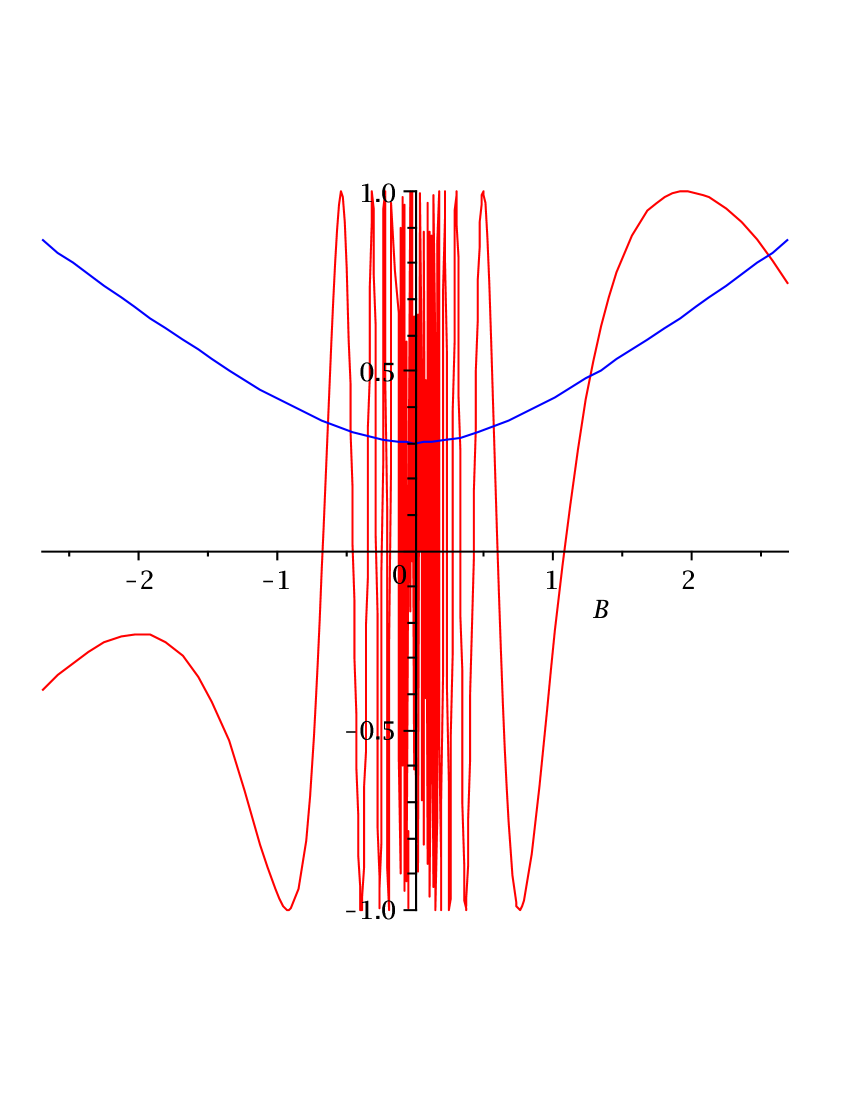
Figure 1. Solutions to the equation (5.5)

However, in order do define the parameters $B$, we need to solve the equations (5.4), (5.5), and not all $B_{n}$ satisfy all three equations. Let us consider positive $B_{n}$. We calculate the argument of $z$ as

$$\alpha=-B_{n}s+\arctan\Bigg{[}\frac{B_{n}}{\sqrt{B_{n}^{2}+1}}\tan\left(s\sqrt{B_{n}^{2}+1}\right)\Bigg{]}$$

$$=-B_{n}s+\arctan\Bigg{[}\frac{B_{n}\rho}{\sqrt{1-(1+B_{n}^{2})\rho^{2}}}\Bigg{]}$$

$$<-B_{n}s+\frac{B_{n}\rho}{\sqrt{1-(1+B_{n}^{2})\rho^{2}}}.$$

On the other hand, we have

$$1=\frac{\arcsin(\rho\sqrt{1+B_{n}^{2}})}{s\sqrt{1+B_{n}^{2}}}>\frac{\rho}{s}.$$

Observe that due the remark before this theorem, $\alpha>0$ and $0<\rho<1$. Therefore, we deduce the inequality

$$\alpha<B_{n}\rho\frac{1-\sqrt{1-\rho^{2}(1+B_{n}^{2})}}{\sqrt{1-\rho^{2}(1+B_{n}^{2})}},$$

or

$$B_{n}\rho>\alpha\frac{\sqrt{1-\rho^{2}(1+B_{n}^{2})}}{1-\sqrt{1-\rho^{2}(1+B_{n}^{2})}}.$$ (5.6)

The right-hand side of the inequality (5.6) decreases with respect to $B_{n}>0$.

Set $\varepsilon=\frac{1+\rho^{2}}{2}$. If $\varepsilon<\rho^{2}(1+B_{n}^{2})<1$, then immediately we have the inequality $B_{n}^{2}>\frac{1}{2}(\frac{1}{\rho^{2}}-1)>0$. If $0<\rho^{2}(1+B_{n}^{2})\leq\varepsilon$, then the inequality (5.6) implies that

$$B_{n}>\alpha\frac{\sqrt{1-\varepsilon}}{\rho(1-\sqrt{1-\varepsilon})}=\alpha\frac{\sqrt{1-\rho^{2}}}{\rho(\sqrt{2}-\sqrt{1-\rho^{2}})}>0.$$

Finally, we obtain

$$B_{n}>\min\left\{\alpha\frac{\sqrt{1-\rho^{2}}}{\rho(\sqrt{2}-\sqrt{1-\rho^{2}})},\sqrt{\frac{1}{2}(\frac{1}{\rho^{2}}-1)}\right\}\equiv b(\xi_{1},\rho)>0.$$

This proves that all positive solutions to the equation (5.5) must belong to the interval $(b(\xi_{1},\rho),\sqrt{\frac{1}{\rho^{2}}-1})$, hence there are only finite number of such $B_{n}$. The same arguments are applied for negative values of $B_{n}$.

Let us discuss the limiting cases. If $\rho\to 0$ then the endpoint aproaches the vertical line. In this case the graph of the right hand side function in (5.5) approaches the horizontal axis and the range of $|B|$ increases. If $\alpha\to 0$ then the end point aproaches the horizontal sphere $\mathbb{S}^{2}$, the number of geodesics is finite for any value $\alpha\neq 0$, but decreases. ∎

This theorem reveals similarity of sub-Riemannian geodesics on the sphere with those for the Heisenberg group. The number of geodesics joining the origin with a point neither from the vertical axis nor from the horizontal plane is finite and approaching the vertical line becomes infinite.

Hyperspherical coordinates

Let us use the hyperspherical coordinates to find geodesics with non-constant velocity coordinates.

$$x_{1}+ix_{2} = e^{i\xi_{1}}\cos\eta,$$ (5.7)

$$x_{3}+ix_{4} = e^{i\xi_{2}}\sin\eta,\qquad\eta\in[0,\pi/2),\quad\xi_{1},\xi_{2}\in[-\pi,\pi)$$

The horizontal coordinates are written as

$$a = \dot{\eta}\cos(\xi_{1}-\xi_{2})+(\dot{\xi}_{1}+\dot{\xi}_{2})\sin(\xi_{1}-\xi_{2})\frac{\sin 2\eta}{2},$$

$$b = -\dot{\eta}\sin(\xi_{1}-\xi_{2})+(\dot{\xi}_{1}+\dot{\xi}_{2})\cos(\xi_{1}-\xi_{2})\frac{\sin 2\eta}{2},$$

$$c = \dot{\xi}_{1}\cos^{2}\eta-\dot{\xi}_{2}\sin^{2}\eta.$$

The horizontality condition in hyperspherical coordinates becomes

$$\dot{\xi}_{1}\cos^{2}\eta-\dot{\xi}_{2}\sin^{2}\eta=0.$$

The horizontal sphere (4.4) is obtained from the parametrization (5.7), if we set $\xi_{1}=0$, $\xi_{2}=\psi$, $\eta=s$. We get

$$a^{2}+b^{2}=1=\dot{\eta}^{2}\quad\Longrightarrow\quad a=\cos\psi,\quad b=\sin\psi.$$

The vertical line is obtained from the parametrization (5.7) setting $\eta=0$, $\xi_{1}=s$.

Writing the vector fields $N,Z,X,Y$ in the hyperspherical coordinates we get

$$N=-2\operatorname{cotan}2\eta\partial_{\eta},\quad Z=\partial_{\xi_{1}}-\partial_{\xi_{2}},$$

$$X=\sin(\xi_{1}-\xi_{2})\tan\eta\partial_{\xi_{1}}+\sin(\xi_{1}-\xi_{2})\operatorname{cotan}\eta\partial_{\xi_{2}}+2\cos(\xi_{1}-\xi_{2})\partial_{\eta},$$

$$Y=\cos(\xi_{1}-\xi_{2})\tan\eta\partial_{\xi_{1}}+\cos(\xi_{1}-\xi_{2})\operatorname{cotan}\eta\partial_{\xi_{2}}-2\sin(\xi_{1}-\xi_{2})\partial_{\eta}.$$

In this parametrization the similarity with the Heisenberg group can be shown. The commutator of two horizontal vector fields $X,Y$ gives the constant vector field $Z$ which is orthogonal to the horizontal vector fields at each point of the manifold. In hyperspherical coordinates it is easy to see that the form $\omega=\cos^{2}\eta d\xi_{1}-\sin^{2}\eta d\xi_{2}$, that defines the horizontal distribution is contact because

$$\omega\wedge d\omega=\sin(2\eta)\,d\eta\wedge d\xi_{1}\wedge d\xi_{2}=2dV,$$

where $dV$ is the volume form. The sub-Laplacian is defined as

$$\frac{1}{2}(X^{2}+Y^{2})=\frac{1}{2}(\tan^{2}\eta\partial^{2}_{\xi_{1}}+\operatorname{cotan}^{2}\eta\partial^{2}_{\xi_{2}}+4\partial^{2}_{\eta}+2\partial_{\xi_{1}}\partial_{\xi_{2}}).$$

The Hamiltonian becomes

$$H(\xi_{1},\xi_{2},\eta,\psi_{1},\psi_{2},\theta)=\frac{1}{2}(\tan^{2}\eta\psi^{2}_{1}+\operatorname{cotan}^{2}\eta\psi^{2}_{2}+4\theta^{2}+2\psi_{1}\psi_{2}),$$

and the corresponding Hamiltonian system is given as

$$\dot{\xi}_{1} = \frac{\partial H}{\partial\psi_{1}}=\psi_{1}\tan^{2}\eta+\psi_{2}$$

$$\dot{\xi}_{2} = \frac{\partial H}{\partial\psi_{2}}=\psi_{2}\operatorname{cotan}^{2}\eta+\psi_{1}$$

$$\dot{\eta} = \frac{\partial H}{\partial\theta}=4\theta$$

$$\dot{\psi}_{1} = -\frac{\partial H}{\partial\xi_{1}}=0$$

$$\dot{\psi}_{2} = -\frac{\partial H}{\partial\xi_{2}}=0$$

$$\dot{\theta} = -\frac{\partial H}{\partial\eta}=-\psi_{1}^{2}\frac{\tan\eta}{\cos^{2}\eta}+\psi_{2}^{2}\frac{\operatorname{cotan}\eta}{\sin^{2}\eta}$$

Let us solve this Hamiltonian system for the following initial data: $\eta(0)=0$, $\xi_{1}(0)=0$, $\xi_{2}(0)=0$, $\psi_{1}(0)=\psi_{1}$, $\psi_{2}(0)=\psi_{2}$, $\theta(0)=\frac{\dot{\eta}(0)}{4}=\theta_{0}$.

We see that $\psi_{1}$ and $\psi_{2}$ are constant. The horizontality condition at $(0,0,0)$ gives $\dot{\xi}(0)=0$ and the first equation of Hamiltonian system implies that $\psi_{2}=0$. If $\psi_{1}=0$, then $\dot{\xi}_{1}=\dot{\xi}_{2}=0$, $\dot{\eta}=4\theta_{0}$ and we get the variety of trivial geodesics (4.4) up to the reparametrization $s\mapsto 4\theta_{0}s$. To find other geodesics we suppose that $\psi_{1}\neq 0$ and $\dot{\eta}(0)>0$. This condition ensures us that the trajectory starting at the point $(0,0,0,)$ remains in the domain of parametrizaition locally in time. From the third and from the last equations of the Hamiltonian system we have

$$\ddot{\eta}=-4\psi_{1}^{2}\frac{\sin\eta}{\cos^{3}\eta}\qquad\Rightarrow\qquad\dot{\eta}\,d\dot{\eta}=-4\psi_{1}^{2}\frac{\sin\eta}{\cos^{3}\eta}d\eta\qquad\Rightarrow$$

$$\dot{\eta}^{2}=C-4\frac{\psi_{1}^{2}}{\cos^{2}\eta},$$

We observe that $C=\dot{\eta}^{2}(0)+4\psi_{1}^{2}>0$.

Continue to solve the Hamiltonian system finding $\eta(s)$.

$$\frac{\cos\eta\,d\eta}{\sqrt{C\cos^{2}\eta-4\psi_{1}^{2}}}=ds.$$

Denote by $\sin\eta=p$. Then,

$$\frac{dp}{\sqrt{-Cp^{2}+C-4\psi_{1}^{2}}}=ds.$$ (5.8)

Integrating (5.8) from $0$ to $s$ we get

$$s+K=\frac{1}{\sqrt{|C|}}\arcsin\Big{(}\sqrt{\frac{C}{C-4\psi_{1}^{2}}}\sin\eta(s)\Big{)},$$

where $K$ is found setting $s=0$ as $K=\frac{1}{\sqrt{|C|}}\arcsin 0=0$. We calculate

$$\sin^{2}\eta(s)=\frac{C-4\psi^{2}_{1}}{C}\sin^{2}(\sqrt{C}s).$$ (5.9)

From the Hamiltonian system we find

$$\xi_{2}(s)=\psi_{1}s,$$ (5.10)

and

$$\dot{\xi}_{1}=\psi_{1}\frac{\sin^{2}\eta(s)}{1-\sin^{2}\eta(s)}=\psi_{1}\frac{\sin^{2}(\sqrt{C}s)}{a+\sin^{2}(\sqrt{C}s)},\quad a=\frac{C}{C-4\psi_{1}^{2}}.$$

It gives

$$\xi_{1}(s)=-\psi_{1}s+\frac{\psi_{1}}{2|\psi_{1}|}\arctan\Big{[}\frac{2|\psi_{1}|}{\sqrt{C}}\tan(\sqrt{C}s)\Big{]}.$$ (5.11)

Let us suppose for the moment that the geodesics are parametrized on the interval $[0,1]$. If the initial point and the finite point are on the vertical line: $\eta(0)=\eta(1)=0$, then

$$0=\sin^{2}\eta(1)=\frac{C-4\psi^{2}_{1}}{C}\sin^{2}(\sqrt{C})\quad\Rightarrow\quad C=\pi^{2}n^{2}.$$

Since the value of $\xi_{2}$ on the vertical line is arbitrary, the values of $C$ and $\xi_{1}(1)$ give us the value of $\xi_{2}(1)$. Setting $C=\pi^{2}n^{2}$ in the equation for $\xi_{1}(1)$, we find $\psi_{1}=-\xi_{1}(1)$. Then

$$\xi_{2}(1)=-\xi_{1}(1).$$

The finite point on the vertical line corresponds to the value of $\xi_{1}(1),\eta(1)=0$, and $\xi_{2}=-\xi_{1}(1)$.

We also note that the square of the velocity $|v|^{2}=\dot{\eta}^{2}(s)+(\dot{\xi}_{1}(s)+\dot{\xi}_{2}(s))^{2}\frac{\sin^{2}2\eta(s)}{2}$ is constant along geodesics. Applying the initial condition $\eta(0)=0$, we get

$$|v|^{2}=\dot{\eta}^{2}(0)=C-4\psi_{1}^{2}.$$

In the case when a geodesic ends at the vertical line at $\xi_{1}(1)$, its lengths is expressed as

$$\sqrt{2}l_{n}=\sqrt{C-4\psi_{1}^{2}}=\sqrt{\pi^{2}n^{2}-4\xi_{1}^{2}(1)}.$$

We see that this result coincides with the result given by Theorem 2 and we state it as follows.

Theorem 4.

Let $A$ be a point of the vertical line, i. e. $\xi_{1}$ is given and $\eta=0$. There are countably many geodesics $\gamma_{n}$ connecting $O=(0,0,0)$ and $A$, given parametrically as

$$\xi_{1}(s) = \xi_{1}s+\frac{1}{2}\arctan\Big{(}\frac{2\xi_{1}}{\pi n}\tan(\pi ns)\Big{)},$$

$$\xi_{2}(s) = -\xi_{1}s,$$

$$\sin\eta(s) = \frac{s_{n}}{\pi n}\sin(\pi ns),$$

where $\frac{1}{\sqrt{2}}s_{n}=\frac{1}{\sqrt{2}}\sqrt{\pi^{2}n^{2}-4\xi_{1}^{2}}$ is the length of the geodesic $\gamma_{n}$, $n\in\mathbb{N}$.

6. Hopf fibration

There is a close relation between the sub-Riemannian sphere $S^{3}$ and the Hopf fibration. Let $\mathbb{S}^{2}$ and $\mathbb{S}^{3}$ be unit 2-dimensional and 3-dimensional sphere respectively. We remind that the Hopf fibration is a principal circle bundle over two-sphere given by the map $h:\mathbb{S}^{3}\to\mathbb{S}^{2}$:

$$h(x_{1},x_{2},x_{3},x_{4})=((x_{1}^{2}+x_{2}^{2})-(x_{3}^{2}+x_{4}^{2}),2(x_{1}x_{4}+x_{2}x_{3}),2(x_{2}x_{4}-x_{1}x_{3})).$$

Another way to define the Hopf fibration is to write

$$h(q)=qiq^{*}\in\mathbb{S}^{2},\quad q\in\mathbb{S}^{3},\quad i=(0,1,0,0).$$

The fiber passing through the unity of the group $(1,0,0,0)$ has equation $(\cos\theta,\sin\theta,0,0)$, which as we see, coincides with the equation of the vertical line at this point. The sphere $\mathbb{S}^{2}$ represents the horizontal “plane” sweep out by the geodesics with constant horizontal coordinates.

Definition 1.

Let $Q\to M$ be a principle $G$-bundle with the horizontal distribution $\mathcal{D}$ on $Q$. A sub-Riemannian metric on $Q$ that has distribution $\mathcal{D}$ and it is invariant under the action of $G$ is called a metric of bundle type.

In our situation $\mathbb{S}^{3}\to\mathbb{S}^{2}$ is a principle $\mathbb{S}^{1}$-bundle given by the Hopf map. The sub-Riemannian metric on the distribution $\mathcal{D}=\operatorname{span}\{X,Y\}$ was defined as the restriction of the euclidean metric $\langle\cdot,\cdot\rangle$ from $\mathbb{R}^{4}$ and we used the same notation $\langle\cdot,\cdot\rangle$ for sub-Riemannian metric.

Proposition 3.

The sub-Riemannian metric $\langle\cdot,\cdot\rangle$ on $\mathbb{S}^{3}$ is a metric of bundle type.

Proof.

The action of the group $\mathbb{S}^{1}$ on $q=(x_{1},x_{2},x_{3},x_{4})\in\mathbb{S}^{3}$ can be written as $q\circ e^{it}$, $e^{it}=(\cos t+i\sin t)\in\mathbb{S}^{1}$, $t\in[0,2\pi)$, where $\circ$ is the quaternion multiplication. If we write $q=(e^{i\xi_{1}}\cos\eta,e^{i\xi_{2}}\sin\eta)$, $\tilde{q}=q\circ e^{it}$, then $\tilde{q}=(e^{i(\xi_{1}+t)}\cos\eta,e^{i(\xi_{2}-t)}\sin\eta)$. In order to show that the metric $\langle\cdot,\cdot\rangle$ is of bundle type, we have to prove that the metric is invariant under the action of the group $\mathbb{S}^{1}$. The metric $\langle\cdot,\cdot\rangle$ at any $q$ is given by the matrix

$$\left[\begin{array}[]{rrr}1&0&0\\ 0&\cos^{2}\eta&0\\ 0&0&\sin^{2}\eta\end{array}\right]$$

and it is easy to see that it is invariant under the action $\tilde{q}=q\circ e^{it}$. ∎

We can formulate the results of Theorems 2 and 4 as an isoholonomic problem. First let us give some definitions. Let $c:[0,1]\to\mathbb{S}^{2}$ be a curve in $\mathbb{S}^{2}$ For a given point $x$ of the fiber $Q_{c(0)}$ at $c(0)$, let $\gamma$ be a horizontal lift of $c$ that starts at $q$ (it means that the projection of $\gamma$ under the Hopf map $h:\mathbb{S}^{3}\to\mathbb{S}^{2}$ coincides with $c$). The map $\Phi(c):Q_{c(0)}\to Q_{c(1)}$ sending $x=\gamma(0)$ to the endpoint $\gamma(1)$ of the horizontal lift is called parallel transport along $c$. The action of $\mathbb{S}^{1}$ takes horizontal curves to horizontal curves, so any two horizontal curves $\gamma_{1}$ and $\gamma_{2}$ of $c$ are related by $\gamma_{1}=\gamma_{2}g$ for some $g\in\mathbb{S}^{1}$. It follows that the action of $\mathbb{S}^{1}$ commutes with $\Phi(c)$, that is, $\Phi(c)(xg)=\big{(}\Phi(c)(x)\big{)}g$.

If $c$ is a closed loop, parallel transport $\Phi(c)$ maps the fiber $Q_{c(0)}$ onto itself. Fix a point $x_{0}\in Q_{c(0)}$. Since $\mathbb{S}^{1}$ acts transitively on $Q_{c(0)}$ we have $\phi(c)(x_{0})=x_{0}l$ for some $l\in\mathbb{S}^{1}$. If we choose another point $y_{0}=x_{0}g\in Q_{c(0)}$, we get

$$\Phi(c)(y_{0})=\big{(}\Phi(c)(x_{0})\big{)}(g)=x_{0}lg=y_{0}(g^{-1}lg).$$

The curve $c$ therefore, determines a conjugacy class in $\mathbb{S}^{1}$, called the holonomy class of $c$. The element $l\in\mathbb{S}^{1}$ for which $\Phi(c)(x_{0})=x_{0}l$ is called the representative holonomy of $c$ with respect to $x_{0}$. The set of all such $l\in\mathcal{S}^{1}$ for $c$ running over all closed loops with $c(0)=c(1)=h(x_{0})$ is a subgroup of $\mathbb{S}^{1}$ called the holonomy group of the distribution $\mathcal{D}$ at $x_{0}$.

Let us fix a representative holonomy $l\in\mathbb{S}^{1}$ and a point $x_{0}\in\mathbb{S}^{3}$, or equivalently the initial and the finite points $x_{0}$ and $x_{1}=x_{0}l$. The set of horizontal curves that join $x_{0}$ to $x_{1}$ is in one-to-one correspondence with the set of all closed loops on $\mathbb{S}^{2}$, based at $h(x_{0})$, whose holonomy with respect to $x_{0}$ is $l$. Recall that the Riemannian length of a loop on $\mathbb{S}^{2}$ equals the sub-Riemannian length of its horizontal lift. Thus, the sub-Riemannian geodesic problem for geodesics with endpoints at the same fiber is equivalent to the following isoholonomic problem: Among all loops with a given holonomy, find the shortest.

If we take $x_{0}=(1,0,0,0)$, $l=e^{i\omega}$, $x_{1}=x_{0}l=(\cos\omega,\sin\omega,0,0)$, then Theorem 2 says

$$\text{if}\quad\omega\in[0,\pi) \quad\text{then the shortest loop has length}\quad s_{1}=\sqrt{\pi^{2}n^{2}-\omega^{2}},$$

$$\text{if}\quad\omega\in[\pi,2\pi) \quad\text{then the shortest loop has length}\quad s_{2}=\sqrt{4\pi^{2}n^{2}-\omega^{2}}.$$