Quantum Heisenberg antiferromagnets in a uniform magnetic field: Non-analytic magnetic field dependence of the magnon spectrum

Abstract

We re-examine the $1/S$-correction to the self-energy of the gapless magnon of a $D$-dimensional quantum Heisenberg antiferromagnet in a uniform magnetic field $h$ using a hybrid approach between $1/S$-expansion and non-linear sigma model, where the Holstein-Primakoff bosons are expressed in terms of Hermitian field operators representing the uniform and the staggered components of the spin-operators [N. Hasselmann and P. Kopietz, Europhys. Lett. 74, 1067 (2006)]. By integrating over the field associated with the uniform spin-fluctuations we obtain the effective action for the staggered spin-fluctuations on the lattice, which contains fluctuations on all length scales and does not have the cutoff ambiguities of the non-linear sigma model. We show that in dimensions $D\leq 3$ the magnetic field dependence of the spin-wave velocity $\tilde{c}_{-}(h)$ is non-analytic in $h^{2}$, with $\tilde{c}_{-}(h)-\tilde{c}_{-}(0)\propto h^{2}\ln|h|$ in $D=3$, and $\tilde{c}_{-}(h)-\tilde{c}_{-}(0)\propto|h|$ in $D=2$. The frequency dependent magnon self-energy is found to exhibit an even more singular magnetic field dependence, implying a strong momentum dependence of the quasi-particle residue of the gapless magnon. We also discuss the problem of spontaneous magnon decay and show that in $D>1$ dimensions the damping of magnons with momentum $\bm{k}$ is proportional to $|\bm{k}|^{2D-1}$ if spontaneous magnon decay is kinematically allowed.

I Introduction

One of the most successful methods for obtaining the low-temperature properties of ordered quantum Heisenberg magnets is the expansion in inverse powers of the spin quantum number $S$. The idea is to first map the spin Hamiltonian onto an interacting boson model using either the Holstein-Primakoff Holstein40 or the Dyson-Maleyev transformation Dyson56 ; Maleyev57 , and then study the resulting interacting boson system by means of the usual many-body machinery. As the interaction vertices appearing in the boson Hamiltonian involve the small parameter of $1/S$, the perturbative treatment of the interaction is formally justified for large $S$. See, for example, Refs. [Oguchi60, ; Harris71, ] for early applications of this approach to quantum antiferromagnets (QAFM). A disadvantage of this method is that calculations for QAFM beyond the leading order in $1/S$ are very tedious due to a large number of interaction vertices Harris71 . Moreover, the vertices are even singular for certain combinations of external momenta Harris71 ; Kopietz90 ; Hasselmann06 . Although the singularities cancel in physical quantities if the total spin is conserved Maleyev00 , the appearance of singularities at intermediate stages of the calculation indicates that this approach is not always the best way of calculating fluctuation corrections to the magnon spectrum.

In this work we shall re-consider the leading $1/S$-correction to the magnon self-energy of spin-$S$ quantum Heisenberg antiferromagnets in a uniform magnetic field $\bm{h}$ at zero temperature in the regime where the system has a finite staggered magnetization. Our starting point is the Heisenberg Hamiltonian

$$\hat{H}=\frac{1}{2}\sum_{ij}J_{ij}\bm{S}_{i}\cdot\bm{S}_{j}-\sum_{i}\bm{h}\cdot\bm{S}_{i},$$ (1)

where $\bm{S}_{i}$ are spin operators normalized such that $\bm{S}_{i}^{2}=S(S+1)$ and the magnetic field $\bm{h}$ is measured in units of energy. The exchange integrals $J_{ij}$ connect nearest neighbor sites ${\bm{r}}_{i}$ and $\bm{r}_{j}$ on a $D$-dimensional hypercubic lattice with lattice spacing $a$, total volume $V=a^{D}N$ and $N$ sites. As long as $|\bm{h}|$ is smaller than a certain critical value $h_{c}$ (see Eq. (21) below), the spin configuration in the ground state is canted, as shown in Fig. 1.

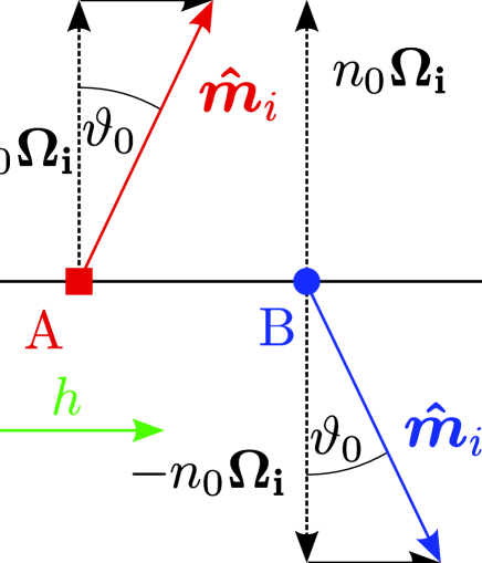
Figure 1: (Color online) Spin configuration $\langle\bm{S}_{i}\rangle=S\hat{\bm{m}}_{i}$ in the classical ground state of a two-sublattice antiferromagnet subject to a uniform magnetic field $\bm{h}=h\bm{e}_{x}$ in the $x$-direction. The hypercubic lattice can be divided into two sublattices, labeled A and B, such that the nearest neighbors of a given site all belong to the other sublattice. The solid square denotes a site of the A-sublattice and a solid circle denotes a site of the B-sublattice. Here $\vartheta_{0}$ is the classical canting angle between the direction of the staggered magnetization $\bm{\Omega}_{i}$ and the local spin direction $\hat{\bm{m}}_{i}$.

We choose our coordinate system such that the magnetic field $\bm{h}=h{\bm{e}}_{x}$ points along the $x$-axis and the staggered magnetization $\bm{M}_{s}=M_{s}{\bm{e}}_{z}$ points in $z$-direction. The magnetic field generates a uniform magnetization $\bm{M}=M{\bm{e}}_{x}$ pointing in the same direction as $\bm{h}$, giving via $\bm{h}$ a gap in the transverse magnon polarized parallel to $\bm{h}$, while the magnon polarized perpendicular to $\bm{h}$ remains gapless.

Due to the canting of the spins, the effective boson Hamiltonian obtained from Eq. (1) within the Holstein-Primakoff transformation contains cubic interaction vertices proportional to $S^{-1/2}$. Hence, to obtain the complete $1/S$-correction to physical observables, the cubic vertices should be treated in second order perturbation theory. The leading $1/S$-corrections to the magnon spectrum turns out to be rather peculiar: Zhitomirsky and Chernyshev Zhitomirsky99 have shown that for intermediate magnetic fields in a certain range $h_{\ast}<|\bm{h}|<h_{c}$ there are no well-defined magnons in a large part of the Brillouin zone due to spontaneous two-magnon decays. Moreover, Syromyatnikov and Maleyev Syromyatnikov01 calculated the $1/S$-correction to the anisotropy induced gap of the magnon polarized parallel to the magnetic field, and showed that in dimensions $D\leq 3$ the correction is unexpectedly large. They suggested that meaningful results can only be obtained if the $1/S$-expansion is re-summed to all orders, which is of course impossible in practice.

Unfortunately, within the conventional $1/S$ expansion, the expressions for the magnon self-energies (see Refs. [Zhitomirsky99, ; Syromyatnikov01, ]) are quite complicated. For example, from the expression for the magnon self-energy given by Zhitomirsky and Chernyshev Zhitomirsky99 (which we reproduce in Appendix B) it is not immediately obvious that one of the magnon branches remains gapless. In this work we shall therefore re-consider this problem using our recently proposed parameterization of the $1/S$-expansion in terms of Hermitian field operators Hasselmann06 . The advantages of such an approach have already been pointed out in Ref. [Hasselmann06, ], but the practical usefulness of this method has not been demonstrated. In a sense, our method is a hybrid approach between the $1/S$-expansion and the non-linear sigma model (NLSM) approach Chakravarty89 ; Fisher89 ; Sachdev99 . Recall that the NLSM is an effective continuum theory for the staggered spin-fluctuations of a QAFM. In contrast to the singular interaction vertices encountered in the conventional $1/S$-expansion, the vertices describing interactions between transverse spin-fluctuations in the NLSM are finite in momentum space and all scale as $\bm{k}^{2}$ for $\bm{h}=0$. On the other hand, the NLSM has to be regularized using an ultraviolet cutoff, so that the NLSM approach cannot be used to obtain the numerical value of observables which receive contributions from wave-vectors in the entire Brillouin zone. Our approach combines the advantages of the $1/S$-expansion with the those of the NLSM by parameterizing the degrees of freedom in the $1/S$-expansion from the beginning in terms of a lattice version of the continuum field representing staggered spin fluctuations in the NLSM.

The rest of this work is organized as follows: After giving a detailed description of our hybrid approach in Sec. II, we derive the effective action for staggered spin fluctuations of our lattice model in Sec. III and exhibit the precise connection with the NLSM, where only the leading orders in the derivatives are retained. In particular, we show how the regular vertices of the NLSM emerge from the conventional $1/S$-expansion. In Sec. IV we then use our method to derive expressions for the frequency dependent part of the magnon self-energies which for small magnetic field $\bm{h}$ determines the dominant $\bm{h}$-dependence of the magnon dispersions. In Sec. V the self-energy of the gapless magnon is evaluated; in particular, we show that in dimensions $D\leq 3$ the fluctuation corrections to the spin-wave velocity and the quasi-particle residue of the gapless magnon exhibit a non-analytic $\bm{h}$-dependence. We also discuss the problem of spontaneous magnon decay in general dimensions. After a brief summary of our results in Sec. VI, we give in Appendix A explicit expressions for the quartic interaction vertices associated with two-magnon scattering in our hybrid approach. Finally in Appendix B we show numerically that in $D=2$ our result for the magnetic field dependency of the spin-wave velocity of the gapless magnon can also be extracted from the self-energy given by Zhitomirsky and Chernyshev in Ref. [Zhitomirsky99, ].

II Hybrid approach: combining the advantages of the $1/S$-expansion with those of the NLSM

II.1 Holstein-Primakoff boson Hamiltonian

For completeness, let us briefly recall the general procedure for setting up the $1/S$-expansion around a given classical ground-state, characterized by the directions $\hat{\bm{m}}_{i}=\langle\bm{S}_{i}\rangle/|\langle\bm{S}_{i}\rangle|$ of the local magnetic moments Schuetz03 . Supplementing the unit vector $\hat{\bm{m}}_{i}$ by two additional unit vectors ${\bm{e}}_{i}^{(1)}$ and ${\bm{e}}_{i}^{(2)}$ such that ${\bm{e}}_{i}^{(1)},{\bm{e}}_{i}^{(2)},\hat{\bm{m}}_{i}$ form a right-handed orthogonal triad of unit vectors, and defining the corresponding spherical basis vectors ${\bm{e}}^{p}_{i}$ $=$ ${\bm{e}}^{(1)}_{i}+ip{\bm{e}}^{(2)}_{i}$, $p$ $=$ $\pm$, we express the components of the spin operator $\bm{S}_{i}$ in terms of canonical boson operators $b_{i}$ and $b_{i}^{\dagger}$ using the Holstein-Primakoff transformation Holstein40 ,

$${\bm{S}}_{i}=S^{\parallel}_{i}\hat{\bm{m}}_{i}+{\bm{S}}^{\bot}_{i}=S^{\parallel}_{i}\hat{\bm{m}}_{i}+\frac{1}{2}\sum_{p=\pm}S_{i}^{-p}{\bm{e}}^{p}_{i}\;,$$ (2)

with

$$S_{i}^{\parallel} = S-n_{i}\;\;,\;\;n_{i}=b^{\dagger}_{i}b_{i}\;,$$ (3a)

$$S_{i}^{+} = \sqrt{2S}\sqrt{1-\frac{n_{i}}{2S}}b_{i}\;,$$ (3b)

$$S_{i}^{-} = \sqrt{2S}b_{i}^{\dagger}\sqrt{1-\frac{n_{i}}{2S}}\;.$$ (3c)

Our spin Hamiltonian (1) can then be written as the following bosonic many-body Hamiltonian Spremo05

$$\hat{H}=E^{\rm cl}_{0}+\hat{H}_{2}^{\parallel}+\hat{H}_{4}^{\parallel}+\hat{H}^{\bot}+\hat{H}^{\prime}\;,$$ (4)

with the classical ground state energy

$$E^{\rm cl}_{0}=\frac{S^{2}}{2}\sum_{ij}J_{ij}\hat{\bm{m}}_{i}\cdot\hat{\bm{m}}_{j}-S\sum_{i}{\bm{h}}\cdot\hat{\bm{m}}_{i},$$ (5)

and

$$\hat{H}_{2}^{\parallel}=-\frac{S}{2}\sum_{ij}J_{ij}\hat{\bm{m}}_{i}\cdot\hat{\bm{m}}_{j}(n_{i}+n_{j})+\sum_{i}{\bm{h}}\cdot\hat{\bm{m}}_{i}n_{i}\;,$$ (6)

$$\hat{H}_{4}^{\parallel} = \frac{1}{2}\sum_{ij}J_{ij}\hat{\bm{m}}_{i}\cdot\hat{\bm{m}}_{j}n_{i}n_{j}\;,$$ (7)

$$\hat{H}^{\bot} = \frac{1}{2}\sum_{ij}J_{ij}{\bm{S}}^{\bot}_{i}\cdot{\bm{S}}^{\bot}_{j}$$ (8)

$$= \frac{1}{8}\sum_{ij}\sum_{pp^{\prime}}J_{ij}(\bm{e}^{p}_{i}\cdot\bm{e}^{p^{\prime}}_{j})S_{i}^{-p}S_{j}^{-p^{\prime}}\,,$$

$$\hat{H}^{\prime} = -\sum_{i}{\bm{S}}^{\bot}_{i}\cdot\bigl{(}{\bm{h}}-\sum_{j}J_{ij}{{S}}_{j}^{\parallel}\hat{\bm{m}}_{j}\bigr{)}$$ (9)

$$= -\sum_{ij}J_{ij}({\bm{S}}_{i}^{\bot}\cdot\hat{\bm{m}}_{j})n_{j}$$

$$-\sum_{i}{\bm{S}}^{\bot}_{i}\cdot\bigl{(}{\bm{h}}-\sum_{j}J_{ij}S\hat{\bm{m}}_{j}\bigr{)}\,.$$

The part $\hat{H}^{\prime}$ of the Hamiltonian describes the coupling between transverse and longitudinal spin fluctuations generated by the uniform magnetic field. Within the Holstein-Primakoff approach, we expand the square roots in Eqs.(3b) and (3c) in powers of $S^{-1}$,

$$S_{i}^{+} = \sqrt{2S}\;\Biggl{[}b_{i}-\frac{n_{i}b_{i}}{4S}+\ldots\Biggr{]},$$ (10a)

$$S_{i}^{-} = \sqrt{2S}\;\Biggl{[}b_{i}^{\dagger}-\frac{b_{i}^{\dagger}n_{i}}{4S}+\ldots\Biggr{]}.$$ (10b)

The boson representation of the operator $\hat{H}^{\bot}$ can then be written as an infinite series of multiple-boson interactions involving even powers of boson operators, while $\hat{H}^{\prime}$ becomes an infinite series of terms involving odd powers of boson operators,

$$\hat{H}^{\bot} = \hat{H}^{\bot}_{2}+\hat{H}^{\bot}_{4}+O(S^{-1})\;,$$ (11)

$$\hat{H}^{\prime} = \hat{H}_{1}+\hat{H}_{3}+O(S^{-1/2})\;,$$ (12)

where the subscripts indicate the number of boson operators. Making the reasonable assumption that the true spin configuration in the ground state resembles the classical one shown in Fig. 1 (but with a renormalized canting angle $\vartheta$), we have

$$\langle\bm{S}_{i}\rangle=|\langle\bm{S}_{i}\rangle|\hat{\bm{m}}_{i}\;,\;\hat{\bm{m}}_{i}=\zeta_{i}n\bm{e}_{z}+m\bm{e}_{x}\;,$$ (13)

where we have chosen $\bm{h}=h{\bm{e}}_{x}$, and the true canting angle $\vartheta$ is related to $n$ and $m$ via $n=\cos\vartheta$ and $m=\sin\vartheta$. Here $\zeta_{i}$ assumes the value $+1$ on one sublattice (which we call the A-sublattice) and $-1$ on the other sublattice (the B-sublattice). A convenient choice of the other members of the local triad is

$${\bm{e}}_{i}^{(1)}=\bm{e}_{y}\;\;,\;\;{\bm{e}}_{i}^{(2)}=-\zeta_{i}n\bm{e}_{x}+m\bm{e}_{z}\;.$$ (14)

The relevant scalar products in this basis are for nearest neighbor sites $i$ and $j$,

$$\hat{\bm{m}}_{i}\cdot\hat{\bm{m}}_{j} = m^{2}-n^{2}=-\alpha\;,$$ (15a)

$${\bm{e}}_{i}^{+}\cdot{\bm{e}}_{j}^{+} = {\bm{e}}_{i}^{-}\cdot{\bm{e}}_{j}^{-}=2n^{2}\;,$$ (15b)

$${\bm{e}}_{i}^{+}\cdot{\bm{e}}_{j}^{-} = {\bm{e}}_{i}^{-}\cdot{\bm{e}}_{j}^{+}=2m^{2}\;,$$ (15c)

$${\bm{e}}_{i}^{+}\cdot\hat{\bm{m}}_{j} = -{\bm{e}}_{i}^{-}\cdot\hat{\bm{m}}_{j}=-2inm\zeta_{i}=-i\lambda\zeta_{i},\hskip 14.22636pt$$ (15d)

$${\bm{h}}\cdot\hat{\bm{m}}_{i} = hm,$$ (15e)

where we have defined

$$\alpha = n^{2}-m^{2}=1-2m^{2}=\cos(2\vartheta),$$ (16)

$$\lambda = 2nm=\sin(2\vartheta).$$ (17)

Then we obtain from Eq. (5),

$$E^{\rm cl}_{0}=-NDJS^{2}\alpha-NShm,$$ (18)

and from Eq. (6),

$$\hat{H}_{2}^{\parallel}=\frac{Z_{h}}{2}h_{c}\sum_{i}n_{i},$$ (19)

where

$$Z_{h}=1+\frac{2m\delta h}{h_{c}},$$ (20)

and we have introduced the notation

$$h_{c} = 4DJS,$$ (21)

$$\delta h = h-h_{c}m.$$ (22)

In the classical limit $S\rightarrow\infty$ the exchange field $h_{c}m$ exactly cancels the external field $h$, so that in this limit $\delta h=0$. However, for finite $S$ the difference $\delta h=h-h_{c}m$ is finite. We shall show in Sec. III that $\delta h$ is actually of the order of $mh_{c}/S$. The longitudinal part $\hat{H}^{\parallel}_{4}$ of the Hamiltonian involving four boson operators is

$$\hat{H}_{4}^{\parallel}=-\frac{\alpha}{2}\sum_{ij}J_{ij}n_{i}n_{j}\;,$$ (23)

and the leading two terms of the transverse part of the Hamiltonian are

$$\hat{H}_{2}^{\bot} = \frac{S}{4}\sum_{ij}J_{ij}[(\bm{e}^{+}_{i}\cdot\bm{e}^{-}_{j})\;b_{i}^{\dagger}b_{j}+(\bm{e}^{-}_{i}\cdot\bm{e}^{+}_{j})\;b_{j}^{\dagger}b_{i}$$

$$\hskip 34.1433pt+(\bm{e}^{+}_{i}\cdot\bm{e}^{+}_{j})\;b_{i}^{\dagger}b_{j}^{\dagger}+(\bm{e}^{-}_{i}\cdot\bm{e}^{-}_{j})\;b_{j}b_{i}]$$

$$= \frac{S}{2}\sum_{ij}J_{ij}[m^{2}(b_{i}^{\dagger}b_{j}+b_{j}^{\dagger}b_{i})+n^{2}(b_{i}^{\dagger}b_{j}^{\dagger}+b_{j}b_{i})]\;,$$

$$\hat{H}_{4}^{\bot} = -\frac{n^{2}}{8}\!\sum_{ij}J_{ij}\left[n_{i}b_{i}b_{j}+b_{i}n_{j}b_{j}+b^{\dagger}_{i}b^{\dagger}_{j}n_{j}+b^{\dagger}_{i}n_{i}b^{\dagger}_{j}\right]$$

$$-\frac{m^{2}}{8}\!\sum_{ij}J_{ij}\left[n_{i}b_{i}b^{\dagger}_{j}+b_{i}b_{j}^{\dagger}n_{j}+b^{\dagger}_{i}n_{i}b_{j}+b^{\dagger}_{i}n_{j}b_{j}\right]\;.$$

Finally, the part $\hat{H}^{\prime}$ of our effective boson Hamiltonian describing the coupling between transverse and longitudinal fluctuations can be written as

$$\hat{H}^{\prime} = \lambda\sum_{ij}J_{ij}\zeta_{i}S_{i}^{(2)}n_{j}+n\delta h\sum_{i}\zeta_{i}S^{(2)}_{i}\,,$$

where we have set $S^{\pm}_{i}=S_{i}^{(1)}\pm iS_{i}^{(2)}$, so that

$$S_{i}^{(1)} = {\bm{e}}_{i}^{(1)}\cdot\bm{S}_{i}=\frac{1}{2}(S_{i}^{+}+S_{i}^{-})\;,$$ (27a)

$$S_{i}^{(2)} = {\bm{e}}_{i}^{(2)}\cdot\bm{S}_{i}=\frac{1}{2i}(S_{i}^{+}-S_{i}^{-}).$$ (27b)

The alternating factor $\zeta_{i}$ in Eq. (LABEL:eq:Hprime2) indicates that this term describes Umklapp scattering across the boundary of the antiferromagnetic Brillouin zone. For our purpose it is sufficient to neglect all terms in the expansion of Eq. (12) involving five and more boson operators, which amounts to retaining only $\hat{H}_{1}$ and $\hat{H}_{3}$. With our choice of basis vectors these can be written as

$$\hat{H}_{1}=n\delta h\frac{\sqrt{2S}}{2i}\sum_{i}\zeta_{i}(b_{i}-b^{\dagger}_{i})\;,$$ (28)

$$\hat{H}_{3}=\lambda\frac{\sqrt{2S}}{2i}\sum_{ij}J_{ij}\zeta_{i}(b_{i}-b_{i}^{\dagger})n_{j}\;.$$ (29)

Let us emphasize that if we use the Dyson-Maleyev transformation Dyson56 ; Maleyev57 to bosonize the spin operators, we obtain a non-Hermitian transverse part $H_{4}^{\bot}$ which differs from Eq. (LABEL:eq:H4bot) while $H_{1}$, $H_{2}$, $H_{3}$, and $H_{4}^{\parallel}$ are the same as above. Since the physical quantities calculated in this work are essentially determined by $H_{3}$ our results do not depend on whether we use the Holstein-Primakoff or the Dyson-Maleyev formalism.

II.2 Linear spin-wave theory

To obtain the magnon spectrum within linear spin-wave theory, we neglect $\hat{H}_{4}^{\parallel}$ and $\hat{H}^{\prime}$, and approximate the transverse part $\hat{H}^{\bot}$ by its quadratic term in the expansion of the spin operators in terms of the boson operators, $\hat{H}^{\bot}\approx\hat{H}_{2}^{\bot}$. We should now diagonalize the quadratic boson Hamiltonian $\hat{H}_{2}=\hat{H}_{2}^{\parallel}+\hat{H}_{2}^{\bot}$. We work in the sublattice basis and Fourier transform the spin- and boson operators on each sublattice separately: for sites $\bm{r}_{i}$ belonging to the A-sublattice we define

$$S_{i}^{(p)} = \sqrt{\frac{2}{N}}\sum_{\bm{k}}e^{i\bm{k}\cdot\bm{r}_{i}}S_{A,\bm{k}}^{(p)}\;,$$ (30)

$$b_{i} = \sqrt{\frac{2}{N}}\sum_{\bm{k}}e^{i\bm{k}\cdot\bm{r}_{i}}A_{\bm{k}}\;,$$ (31)

and for sites $\bm{r}_{j}$ belonging to the B-sublattice,

$$S_{j}^{(p)} = \sqrt{\frac{2}{N}}\sum_{\bm{k}}e^{i\bm{k}\cdot\bm{r}_{j}}S_{B,\bm{k}}^{(p)}\;,$$ (32)

$$b_{j} = \sqrt{\frac{2}{N}}\sum_{\bm{k}}e^{i\bm{k}\cdot\bm{r}_{j}}B_{\bm{k}}\;,$$ (33)

where the wave-vector sums are over the reduced (antiferromagnetic) Brillouin zone. The quadratic part $\hat{H}_{2}=\hat{H}_{2}^{\parallel}+\hat{H}_{2}^{\bot}$ of our effective boson Hamiltonian becomes

$$\hat{H}_{2} = \tilde{J}_{0}S\sum_{\bm{k}}\bigl{[}Z_{h}(A^{\dagger}_{\bm{k}}A_{\bm{k}}+B^{\dagger}_{\bm{k}}B_{\bm{k}})$$ (34)

$$\hskip 28.45274pt+n^{2}\gamma_{\bm{k}}(B_{-\bm{k}}A_{\bm{k}}+A^{\dagger}_{\bm{k}}B^{\dagger}_{-\bm{k}})$$

$$\hskip 28.45274pt+m^{2}\gamma_{\bm{k}}(B^{\dagger}_{\bm{k}}A_{\bm{k}}+A^{\dagger}_{\bm{k}}B_{\bm{k}})\bigr{]}\;,$$

where $\gamma_{\bm{k}}=\tilde{J}_{\bm{k}}/\tilde{J}_{0}$ with

$$\tilde{J}_{\bm{k}}=\frac{1}{N}\sum_{ij}e^{-i{\bm{k}}\cdot({\bm{r}}_{i}-{\bm{r}}_{j})}J_{ij}.$$ (35)

Note that

$$\tilde{J}_{0}S=2DJS=h_{c}/2.$$ (36)

To completely diagonalize $\hat{H}_{2}$ we first introduce the symmetric and antisymmetric combinations

$$C_{\bm{k}\sigma}=\frac{1}{\sqrt{2}}\left[{A}_{\bm{k}}+\sigma B_{\bm{k}}\right]\;\;,\;\;\sigma=\pm 1\;,$$ (37)

and then perform a Bogoliubov transformation,

$$\left(\begin{array}[]{c}C_{\bm{k}\sigma}\\ C^{\dagger}_{-\bm{k}\sigma}\end{array}\right)=\left(\begin{array}[]{cc}u_{\bm{k}\sigma}&-\sigma v_{\bm{k}\sigma}\\ -\sigma v_{\bm{k}\sigma}&u_{\bm{k}\sigma}\end{array}\right)\left(\begin{array}[]{c}\hat{\Psi}_{\bm{k}\sigma}\\ \hat{\Psi}^{\dagger}_{-\bm{k}\sigma}\end{array}\right)\;,$$ (38)

where

$$u_{\bm{k}\sigma} = \sqrt{\frac{Z_{h}+\sigma m^{2}\gamma_{\bm{k}}+\epsilon_{\bm{k}\sigma}}{2\epsilon_{\bm{k}\sigma}}}\;,$$ (39a)

$$v_{\bm{k}\sigma} = \sqrt{\frac{Z_{h}+\sigma m^{2}\gamma_{\bm{k}}-\epsilon_{\bm{k}\sigma}}{2\epsilon_{\bm{k}\sigma}}}\;,$$ (39b)

with

$$\epsilon_{\bm{k}\sigma} = \Bigl{[}(Z_{h}+\sigma m^{2}\gamma_{\bm{k}})^{2}-(n^{2}\gamma_{\bm{k}})^{2}\Bigr{]}^{1/2}$$ (40)

$$= \bigl{[}Z_{h}+\sigma\gamma_{\bm{k}}\bigr{]}^{1/2}\bigl{[}Z_{h}-\sigma\alpha\gamma_{\bm{k}}\bigr{]}^{1/2}.\hskip 28.45274pt$$

Note that

$$u^{2}_{\bm{k}\sigma}+v^{2}_{\bm{k}\sigma} = \frac{Z_{h}+\sigma m^{2}\gamma_{\bm{k}}}{\epsilon_{\bm{k}\sigma}},$$ (41)

$$2u_{\bm{k}\sigma}v_{\bm{k}\sigma} = \frac{n^{2}\gamma_{\bm{k}}}{\epsilon_{\bm{k}\sigma}}.$$ (42)

Within linear spin-wave theory $\delta h=0$ and hence $Z_{h}=1$, but the factor $Z_{h}$ will deviate from unity if we take higher orders in $1/S$ into account. Since the above transformations are canonical, our magnon operators $\hat{\Psi}_{\bm{k}\sigma}$ satisfy the usual bosonic commutation relations,

$$[\hat{\Psi}_{\bm{k}\sigma},\hat{\Psi}^{\dagger}_{\bm{k}^{\prime}\sigma^{\prime}}]=\delta_{\bm{k},\bm{k}^{\prime}}\delta_{\sigma,\sigma^{\prime}}\;.$$ (43)

In terms of the new operators $\hat{\Psi}_{\bm{k}\sigma}$ the quadratic spin-wave Hamiltonian $\hat{H}_{2}$ is diagonal,

$$\hat{H}_{2}=\sum_{\bm{k}\sigma}E_{\bm{k}\sigma}\Bigl{[}\hat{\Psi}^{\dagger}_{\bm{k}\sigma}\hat{\Psi}_{\bm{k}\sigma}+\frac{1}{2}\Bigr{]}+E_{0\parallel}^{(1)},$$ (44)

with the magnon dispersions

$$E_{\bm{k}\sigma}=\tilde{J}_{0}S\epsilon_{\bm{k}\sigma}.$$ (45)

The constant

$$E_{0\parallel}^{(1)}=-\frac{N}{2}Z_{h}\tilde{J}_{0}S=-NDJS^{2}\frac{Z_{h}}{S}$$ (46)

is the $1/S$-correction to the ground state energy due to longitudinal spin fluctuations. The total $1/S$-correction to the ground state energy is obtained by adding the zero-point energy of the transverse spin-waves to $E_{0\parallel}^{(1)}$,

$$E_{0}^{(1)} = E_{0\parallel}^{(1)}+\frac{1}{2}\sum_{\bm{k}\sigma}E_{\bm{k}\sigma}$$ (47)

$$= -NDJS^{2}\frac{C_{1}(h)}{S},$$

with

$$C_{1}(h)=\frac{1}{N}\sum_{\bm{k}\sigma}(Z_{h}-\epsilon_{\bm{k}\sigma}).$$ (48)

In the long-wavelength limit we obtain to linear order in $\delta h=h-h_{c}m$ and to quadratic order in $\bm{k}$,

$$E_{\bm{k}+}^{2} = mh_{c}h+c_{+}^{2}\bm{k}^{2},$$ (49a)

$$E_{\bm{k}-}^{2} = n^{2}mh_{c}\delta h+c_{-}^{2}\bm{k}^{2}.\hskip 28.45274pt$$ (49b)

For small $m$ the spin-wave velocities are

$$c_{+}^{2} = c_{0}^{2}(1-3m^{2}),$$ (50a)

$$c_{-}^{2} = c_{0}^{2}(n^{2}+2m^{3}\delta h/h_{c}),$$ (50b)

where $c_{0}$ is the leading large-$S$ result for spin-wave velocity for $h=0$,

$$c_{0}=2\sqrt{D}JSa.$$ (51)

At the level of linear spin-wave theory we may approximate the canting angle by its classical value $\vartheta_{0}$, which is determined by the condition $\delta h=0$, or equivalently

$$m=\sin\vartheta_{0}=h/h_{c}.$$ (52)

This result can also be obtained by minimizing the classical energy $E_{0}^{\rm cl}$ in Eq. (5). The gap of the dispersion $E_{\bm{k}+}$ is then simply given by $h$, while the dispersion $E_{\bm{k}-}$ is gapless with spin-wave velocity

$$c_{-}=c_{0}n=c_{0}\sqrt{1-\frac{h^{2}}{h_{c}^{2}}}.$$ (53)

II.3 Hermitian field operators

In the usual $1/S$-approach one now substitutes the relations between the original Holstein-Primakoff bosons $b_{i}$ and the magnon-operators $\hat{\Psi}_{\bm{k}\sigma}$ into Eqs. (23, LABEL:eq:H4bot, 28, 29). This yields rather lengthy expressions involving momentum dependent vertices. However, if one is only interested in the transverse staggered spin fluctuations, it is better perform another transformation which separates the staggered from the uniform spin fluctuations. Therefore we express the magnon operators $\hat{\Psi}_{\bm{k}\sigma}$ in terms of two Hermitian field operators $\hat{X}_{\bm{k}\sigma}$ and $\hat{P}_{\bm{k}\sigma}$ achieving the natural normalization on a lattice as follows Hasselmann06 ; Hasselmann07 ; Anderson52 ,

$$\hat{\Psi}_{\bm{k}\sigma}=p_{\sigma}\left[\sqrt{\frac{{\nu}_{\bm{k}\sigma}}{2}}\hat{X}_{\bm{k}\sigma}+\frac{i}{\sqrt{2{\nu}_{\bm{k}\sigma}}}\hat{P}_{\bm{k}\sigma}\right],$$ (54)

where the phase factors $p_{+}=-i$ and $p_{-}=1$ are chosen for later convenience. Here the dimensionless factors $\nu_{\bm{k}\sigma}$ are defined by

$$\nu_{\bm{k}\sigma}=\frac{E_{\bm{k}\sigma}}{\Delta_{\bm{k}\sigma}},$$ (55)

where

$$\Delta_{\bm{k}\sigma}=2\tilde{J}_{0}Sz_{\bm{k}\sigma}=h_{c}z_{\bm{k}\sigma},$$ (56)

and

$$z_{\bm{k}\sigma} = [u_{\bm{k}\sigma}+v_{\bm{k}\sigma}]^{2}\epsilon_{\bm{k}\sigma}/2$$ (57)

$$= [Z_{h}+(n^{2}+\sigma m^{2})\gamma_{\bm{k}}]/2.$$

Note that $Z_{h}=1$ to leading order in $1/S$, so that to this order

$$z_{\bm{k}+} = (1+\gamma_{\bm{k}})/2,$$ (58a)

$$z_{\bm{k}-} = (1+\alpha\gamma_{\bm{k}})/2,$$ (58b)

where $\alpha=n^{2}-m^{2}$. In particular, for $\bm{k}\rightarrow 0$ we have $z_{\bm{k}+}\rightarrow 1$ and $z_{{\bm{k}}-}\rightarrow(1+\alpha)/2=n^{2}$. One easily verifies the canonical commutation relations,

$$[\hat{X}_{\bm{k}\sigma},\hat{P}_{\bm{k}^{\prime}\sigma^{\prime}}]=i\delta_{\bm{k},-\bm{k}^{\prime}}\delta_{\sigma,\sigma^{\prime}}.$$ (59)

The quadratic part of the spin-wave Hamiltonian can then be written as

$$\hat{H}_{2} = \frac{1}{2}\sum_{\bm{k}\sigma}\Delta_{\bm{k}\sigma}\Bigl{[}\hat{P}_{-\bm{k}\sigma}\hat{P}_{\bm{k}\sigma}+\nu_{\bm{k}\sigma}^{2}\hat{X}_{-\bm{k}\sigma}\hat{X}_{\bm{k}\sigma}\Bigr{]}+E_{0\parallel}^{(1)}.$$

In contrast to the lattice normalization of Eq. (54) in Ref. [Hasselmann07, ] we focused on the continuum limit to exhibit the relation with the NLSM. In that case a continuum normalization of the fields is more convenient,

$$\hat{\Psi}_{\bm{k}\sigma}=p_{\sigma}\sqrt{\frac{\chi_{0}}{2VE_{\bm{k}\sigma}}}\left[E_{\bm{k}\sigma}\hat{\Pi}_{\bm{k}\sigma}+i\chi_{0}^{-1}\hat{\Phi}_{\bm{k}\sigma}\right],$$ (61)

where $\chi_{0}=(2\tilde{J}_{0}a^{D})^{-1}$ is the large-$S$ limit of the uniform transverse susceptibility for $h=0$. The continuum fields fulfill the commutation relation

$$[\hat{\Pi}_{\bm{k}\sigma},\hat{\Phi}_{\bm{k}^{\prime}\sigma^{\prime}}]=iV\delta_{\bm{k},-\bm{k}^{\prime}}\delta_{\sigma,\sigma^{\prime}}.$$ (62)

The relation between lattice and continuum normalizations is

$$\hat{\Pi}_{\bm{k}\sigma} = a^{D}\sqrt{\frac{N}{Sz_{\bm{k}\sigma}}}\hat{X}_{\bm{k}\sigma},$$ (63)

$$\hat{\Phi}_{\bm{k}\sigma} = \sqrt{NSz_{\bm{k}\sigma}}\hat{P}_{\bm{k}\sigma}.$$ (64)

Our spin-wave Hamiltonian (44) in continuum normalization can be written as

$$\hat{H}_{2} = \frac{1}{2V}\!\sum_{\bm{k}\sigma}\Bigl{[}\chi_{0}^{-1}\hat{\Phi}_{-\bm{k}\sigma}\hat{\Phi}_{\bm{k}\sigma}+\chi_{0}E_{\bm{k}\sigma}^{2}\hat{\Pi}_{-\bm{k}\sigma}\hat{\Pi}_{\bm{k}\sigma}\Bigr{]}+E_{0\parallel}^{(1)}.$$

The field $\hat{\Pi}_{\bm{k}\sigma}$ corresponds precisely to the continuum field representing transverse staggered spin fluctuations in the non-linear sigma model Chakravarty89 . However, here we would like to calculate also short-wavelength properties on a lattice, so that we shall work with the lattice normalization (54).

II.4 Spin-wave interactions

In order carry out the $1/S$-expansion using the operators $X_{\bm{k}\sigma}$ and $P_{\bm{k}\sigma}$ defined in Eq. (54), we should first express the interaction part of the bosonized Hamiltonian in terms of these operators. To obtain the leading $1/S$-correction to linear spin-wave theory, it is sufficient to approximate the effective bosonized Hamiltonian by

$$\hat{H}\approx E^{\rm cl}_{0}+\hat{H}_{1}+\hat{H}_{2}+\hat{H}_{3}+\hat{H}_{4}\;,$$ (66)

where $\hat{H}_{4}=\hat{H}_{4}^{\parallel}+\hat{H}_{4}^{\bot}$. Later we shall use the phase space path integral to derive the effective action for staggered fluctuations. All expressions in the Hamiltonian should therefore be symmetrized whenever powers of non-commutating operators are encountered Schulman81 ; Negele88 ; Gollisch01 . Only after symmetrization we may replace the field operators by numbers. If $\hat{A}_{1}\hat{A}_{2}\cdots\hat{A}_{n}$ is a product of operators consisting of $\hat{X}_{{\bm{k}}\sigma}$ or $\hat{P}_{\bm{k}\sigma}$ in arbitrary order, the symmetrized product is

$$\bigl{\{}\hat{A}_{1}\hat{A}_{2}\cdots\hat{A}_{n}\bigr{\}}\equiv\frac{1}{n!}\sum_{P}\hat{A}_{P_{1}}\hat{A}_{P_{2}}\cdots\hat{A}_{P_{n}},$$ (67)

where the sum is over all $n!$ permutations of $1,\ldots,n$. We obtain from Eq. (28) for the linear part of the Hamiltonian,

$$\hat{H}_{1} = n\delta h\sqrt{SN}\hat{P}_{0-}.$$ (68)

The part $\hat{H}_{3}$ in Eq. (29) can be written as

$$\hat{H}_{3} = -\sqrt{\frac{N}{2}}\frac{h_{c}\lambda}{\sqrt{8S}}\hat{P}_{0-}+\sqrt{\frac{2}{N}}\sum_{\bm{k}_{1}\bm{k}_{2}\bm{k}_{3}}\delta_{\bm{k}_{1}+\bm{k}_{2}+\bm{k}_{3},0}$$ (69)

$$\times \Biggr{[}\frac{1}{2!}\Gamma^{PXX}_{---}(\bm{k}_{1};\bm{k}_{2},\bm{k}_{3})\bigl{\{}\hat{P}_{\bm{k}_{1}-}\hat{X}_{\bm{k}_{2}-}\hat{X}_{\bm{k}_{3}-}\bigr{\}}$$

$$+\frac{1}{2!}\Gamma^{PXX}_{-++}(\bm{k}_{1};\bm{k}_{2},\bm{k}_{3})\hat{P}_{\bm{k}_{1}-}\hat{X}_{\bm{k}_{2}+}\hat{X}_{\bm{k}_{3}+}$$

$$+\Gamma^{PXX}_{++-}(\bm{k}_{1};\bm{k}_{2};\bm{k}_{3})\bigl{\{}\hat{P}_{\bm{k}_{1}+}\hat{X}_{\bm{k}_{2}+}\bigr{\}}\hat{X}_{\bm{k}_{3}-}$$

$$+\frac{1}{2!}\Gamma^{PPP}_{-++}(\bm{k}_{1};\bm{k}_{2},\bm{k}_{3})\hat{P}_{\bm{k}_{1}-}\hat{P}_{\bm{k}_{2}+}\hat{P}_{\bm{k}_{3}+}$$

$$+\frac{1}{3!}\Gamma^{PPP}_{---}(\bm{k}_{1},\bm{k}_{2},\bm{k}_{3})\hat{P}_{\bm{k}_{1}-}\hat{P}_{\bm{k}_{2}-}\hat{P}_{\bm{k}_{3}-}\Biggl{]},$$

where the vertices are

$$\Gamma^{PXX}_{---}(\bm{k}_{1};\bm{k}_{2},\bm{k}_{3}) = \frac{h_{c}\lambda}{\sqrt{8S}}\gamma_{\bm{k}_{1}},$$ (70a)

$$\Gamma^{PXX}_{-++}(\bm{k}_{1};\bm{k}_{2},\bm{k}_{3}) = \frac{h_{c}\lambda}{\sqrt{8S}}\left[\gamma_{\bm{k}_{1}}-\gamma_{\bm{k}_{2}}-\gamma_{\bm{k}_{3}}\right],\hskip 28.45274pt$$ (70b)

$$\Gamma^{PXX}_{++-}(\bm{k}_{1};\bm{k}_{2};\bm{k}_{3}) = \frac{h_{c}\lambda}{\sqrt{8S}}\gamma_{\bm{k}_{2}},$$ (70c)

$$\Gamma^{PPP}_{-++}(\bm{k}_{1};\bm{k}_{2},\bm{k}_{3}) = \frac{h_{c}\lambda}{\sqrt{8S}}\gamma_{\bm{k}_{1}},$$ (70d)

$$\Gamma^{PPP}_{---}(\bm{k}_{1},\bm{k}_{2},\bm{k}_{3}) = \frac{h_{c}\lambda}{\sqrt{8S}}\left[\gamma_{\bm{k}_{1}}+\gamma_{\bm{k}_{2}}+\gamma_{\bm{k}_{3}}\right].$$ (70e)

Explicitly, the symmetrized products in Eq. (69) are

$$\bigl{\{}\hat{P}_{1}\hat{X}_{2}\bigr{\}} = \frac{1}{2}\left[\hat{P}_{1},\hat{X}_{2}\right]_{+},$$ (71)

$$\bigl{\{}\hat{P}_{1}\hat{X}_{2}\hat{X}_{3}\bigr{\}} = \frac{1}{3}(\hat{P}_{1}\hat{X}_{2}\hat{X}_{3}+\hat{X}_{2}\hat{X}_{3}\hat{P}_{1})$$ (72)

$$+ \frac{1}{6}(\hat{X}_{2}\hat{P}_{1}\hat{X}_{3}+\hat{X}_{3}\hat{P}_{1}\hat{X}_{2})$$

$$= \frac{1}{2}\left[\hat{P}_{1},\hat{X}_{2}\hat{X}_{3}\right]_{+},$$

where $[\hat{A}_{1},\hat{A}_{2}]_{+}=\hat{A}_{1}\hat{A}_{2}+\hat{A}_{2}\hat{A}_{1}$ is the anti-commutator and we have abbreviated $\hat{P}_{\bm{k}_{1}}$ by $\hat{P}_{1}$ and analogously for the other labels.

Finally, consider the part $\hat{H}_{4}=\hat{H}_{4}^{\parallel}+\hat{H}_{4}^{\bot}$ of the Hamiltonian involving four boson operators, which according to Eqs. (23) and (LABEL:eq:H4bot) is given by

$$\hat{H}_{4} = -\frac{n^{2}}{2}\sum_{ij}J_{ij}\Biggl{\{}n_{i}n_{j}+\frac{1}{4}\bigl{[}n_{i}b_{i}b_{j}+b_{i}n_{j}b_{j}$$ (73)

$$\hskip 28.45274pt+b^{\dagger}_{i}b^{\dagger}_{j}n_{j}+b^{\dagger}_{i}n_{i}b^{\dagger}_{j}\bigr{]}\Biggr{\}}$$

$$+\frac{m^{2}}{2}\sum_{ij}J_{ij}\Biggl{\{}n_{i}n_{j}-\frac{1}{4}\bigl{[}n_{i}b_{i}b^{\dagger}_{j}+b_{i}b_{j}^{\dagger}n_{j}$$

$$\hskip 28.45274pt+b^{\dagger}_{i}n_{i}b_{j}+b^{\dagger}_{i}n_{j}b_{j}\bigr{]}\Biggr{\}}.$$

Expressing $\hat{H}_{4}$ in terms of the operators $\hat{P}_{\bm{k}\sigma}$ and $\hat{X}_{\bm{k}\sigma}$ defined in Eq. (54) and symmetrizing all expressions containing non-commuting operators we obtain

$$\hat{H}_{4}=E_{0\parallel}^{(2)}+\delta\hat{H}_{2}^{\prime}+\hat{H}_{4}^{\prime},$$ (74)

where

$$E_{0\parallel}^{(2)}=-\frac{NDJS^{2}\alpha}{(2S)^{2}}$$ (75)

is a $1/S^{2}$-correction to the classical ground state energy, and

$$\delta\hat{H}_{2}^{\prime}=\frac{1}{2}\sum_{\bm{k}\sigma}\Bigl{[}\Gamma^{P}_{\sigma}(\bm{k})\hat{P}_{-\bm{k}\sigma}\hat{P}_{\bm{k}\sigma}+\Gamma^{X}_{\sigma}(\bm{k})\hat{X}_{-\bm{k}\sigma}\hat{X}_{\bm{k}\sigma}\Bigr{]},$$ (76)

is a $1/S$-correction to $\hat{H}_{2}$. The vertices are

$$\Gamma^{P}_{\sigma}(\bm{k}) = \frac{h_{c}}{4S}\alpha(1+\sigma\gamma_{\bm{k}}),$$ (77a)

$$\Gamma^{X}_{\sigma}(\bm{k}) = \frac{h_{c}}{4S}(\alpha-\sigma\gamma_{\bm{k}}).$$ (77b)

Finally, the properly symmetrized quartic part $\hat{H}_{4}^{\prime}$ of our spin-wave Hamiltonian is given in Appendix A. For our purpose it is only important that the corresponding interaction vertices are non-singular functions of the external momenta and are analytic functions of $h^{2}$.

III Effective action for the staggered spin fluctuations

In Ref. [Hasselmann06, ] the precise relation between the magnon quasi-particle operators of the $1/S$-expansion and the continuum fields $\Pi_{\bm{k}\sigma}$ representing transverse fluctuations of the staggered magnetization has been established. In this section we shall use this relation to derive the effective action for the staggered spin fluctuations for the Hamiltonian (1) retaining sub-leading $1/S$-corrections and short wave length fluctuations in the entire Brillouin zone.

For weak magnetic fields, the operators $\hat{P}_{\sigma}$ correspond to transverse fluctuations of the total spin, while $\hat{X}_{\sigma}$ describe staggered (antiferromagnetic) spin fluctuations. To calculate the self-energy of antiferromagnetic magnons, we can therefore eliminate the degrees of freedom associated with the generalized momenta $\hat{P}_{\sigma}$. This is most conveniently done using path integration. The appropriate path integral in our case is the imaginary time phase space path integral Schulman81 ; Negele88 . Recall that for a one-dimensional quantum mechanical system with position operator $\hat{X}$, momentum operator $\hat{P}$, and Hamiltonian $\hat{H}(\hat{P},\hat{X})$ the partition function can be written as

$${\cal{Z}}=\int{\cal{D}}[P,X]\exp\left\{\int_{0}^{\beta}d\tau\left[iP\frac{\partial X}{\partial\tau}-H_{s}(P,X)\right]\right\}\;,$$ (78)

where $H_{s}(P,X)$ is obtained from the Hamiltonian $\hat{H}(\hat{P},\hat{X})$ by first symmetrizing $\hat{H}(\hat{P},\hat{X})$ with respect to the ordering of the operators $\hat{X}$ and $\hat{P}$, and then replacing the operators by their eigenvalues. In principle, ambiguities associated with the operator ordering in the phase space path integral can always be resolved by going back to the discretized definition of the path integral Schulman81 ; Negele88 . However, recently Gollisch and Wetterich Gollisch01 ; Wetterich07 showed that in the continuum notation the symmetrization prescription leads to the same result as the more fundamental discretized definition of the phase space path integral. The Euclidean action corresponding to our spin-wave Hamiltonian is of the form

$$S[P_{\sigma},X_{\sigma}]=\sum_{l=0}^{\infty}S_{l}[P_{\sigma},X_{\sigma}]\;,$$ (79)

where $S_{l}[P_{\sigma},X_{\sigma}]$ contains $l$ powers of the fields. To obtain the effective action $S_{\rm eff}[X_{\sigma}]$ for the staggered fluctuations, we integrate over the generalized momenta,

$$e^{-S_{\rm eff}[X_{\sigma}]}=\int{\cal{D}}[P_{\sigma}]e^{-S[P_{\sigma},X_{\sigma}]}.$$ (80)

Within the Gaussian approximation (corresponding to linear spin-wave theory) we truncate the expansion (79) at the term $l=2$. The relevant contributions to $S[P_{\sigma},X_{\sigma}]$ can be written as

$$S_{0} = \beta[E^{\rm cl}_{0}+E_{0\parallel}^{(1)}],$$ (81)

$$S_{1}[P_{-}] = \beta n\delta h\sqrt{SN}P_{0-},$$ (82)

and

$$S_{2}[P_{\sigma},X_{\sigma}] = \frac{\beta}{2}\sum_{K,\sigma}\Bigl{[}\Delta_{\bm{k}\sigma}\left(P_{-K\sigma}P_{K\sigma}+\nu_{\bm{k}\sigma}^{2}X_{-K\sigma}X_{K\sigma}\right)$$ (83)

$$\hskip 14.22636pt-\omega(P_{-K\sigma}X_{K\sigma}-X_{-K\sigma}P_{K\sigma})\Bigr{]},$$

where the last term in Eq. (83) corresponds to the measure term $iP\partial X/\partial\tau$ in the phase space functional integral (78). The fields $P_{K\sigma}$ and $X_{K\sigma}$ are defined by replacing the operators $\hat{P}_{\bm{k}\sigma}$ and $\hat{X}_{\bm{k}\sigma}$ by quantum fields $P_{\bm{k}\sigma}(\tau)$ and $X_{\bm{k}\sigma}(\tau)$ depending on imaginary time $\tau$ and expanding the fields in frequency space,

$$P_{\bm{k}\sigma}(\tau) = \sum_{\omega}e^{-i\omega\tau}P_{K\sigma},$$ (84a)

$$X_{\bm{k}\sigma}(\tau) = \sum_{\omega}e^{-i\omega\tau}X_{K\sigma}.$$ (84b)

We combine momenta $\bm{k}$ and bosonic Matsubara frequencies $i\omega$ to form a composite label $K=(\bm{k},i\omega)$. In general the canting angle can be determined from the condition that the functional average of the field $P_{K=0,-}$ vanishes,

$$\langle P_{0-}\rangle=0.$$ (85)

Eq. (85) defines the correction $\delta h=h-h_{c}m=h-h_{c}\sin\vartheta$ and hence the sine of the renormalized canting angle $\sin\vartheta=m=(h-\delta h)/h_{c}$. Within the Gaussian approximation this implies $\delta h=0$, leading to the classical result (52). Hence $S_{1}[P_{-}]=0$ within this approximation and the effective action for the fields $X_{\sigma}$ is given by the Gaussian integral

$$e^{-S_{{\rm eff}}[X_{\sigma}]}\approx e^{-S_{0}}\int{\cal{D}}[P_{\sigma}]e^{-S_{2}[P_{\sigma},X_{\sigma}]}.$$ (86)

Carrying out the integration, we obtain in Gaussian approximation $S_{{\rm eff}}[X_{\sigma}]=S_{0}+S_{{\rm eff}}^{(0)}[X_{\sigma}]$, where

$$S_{{\rm eff}}^{(0)}[X_{\sigma}] = \frac{\beta}{2}\sum_{K\sigma}\frac{E_{\bm{k}\sigma}^{2}+\omega^{2}}{\Delta_{\bm{k}\sigma}}X_{-K\sigma}X_{K\sigma}.$$ (87)

At long wavelengths this action has the same form as the corresponding Gaussian part of the action of the NLSM. However, in contrast to the NLSM, our action is defined on the lattice so that fluctuations on all wavelengths are included. The Gaussian propagator of the $X_{\sigma}$-field is thus

$$\langle X_{K\sigma}X_{K^{\prime}\sigma^{\prime}}\rangle_{0}=\delta_{K,-K^{\prime}}\delta_{\sigma\sigma^{\prime}}(\beta\Delta_{\bm{k}\sigma})^{-1}\frac{\Delta_{\bm{k}\sigma}^{2}}{E_{\bm{k}\sigma}^{2}+\omega^{2}}.$$ (88)

The other propagators are within Gaussian approximation

$$\langle P_{K\sigma}P_{K^{\prime}\sigma^{\prime}}\rangle_{0} = \delta_{K,-K^{\prime}}\delta_{\sigma\sigma^{\prime}}(\beta\Delta_{\bm{k}\sigma})^{-1}\frac{E_{\bm{k}\sigma}^{2}}{E_{\bm{k}\sigma}^{2}+\omega^{2}},\hskip 19.91692pt$$ (89)

$$\langle X_{K\sigma}P_{K^{\prime}\sigma^{\prime}}\rangle_{0} = \delta_{K,-K^{\prime}}\delta_{\sigma\sigma^{\prime}}(\beta\Delta_{\bm{k}\sigma})^{-1}\frac{\Delta_{\bm{k}\sigma}\omega}{E_{\bm{k}\sigma}^{2}+\omega^{2}}.$$ (90)

Here the symbol $\langle\ldots\rangle_{0}$ denotes functional averaging with the Gaussian action $S_{2}[P_{\sigma},X_{\sigma}]$. Note that the formal sum $\sum_{\omega}\langle X_{K\sigma}P_{-K\sigma}\rangle_{0}$ represents the expectation value of the symmetric operator $\langle\{\hat{X}_{\bm{k}\sigma}\hat{P}_{\bm{k}\sigma}\}\rangle_{0}=0$, so that we should regularize formally divergent Matsubara sums using a symmetric convergence factor $\cos(\omega 0^{+})$,

$$\langle\{\hat{X}_{\bm{k}\sigma}\hat{P}_{\bm{k}\sigma}\}\rangle_{0}=\frac{1}{\beta}\sum_{\omega}\frac{\omega\cos(\omega 0^{+})}{E_{\bm{k}\sigma}^{2}+\omega^{2}}=0.$$ (91)

The higher $1/S$-corrections to $S_{\rm eff}[X_{\sigma}]$, can now be obtained by including the spin-wave interactions perturbatively. Therefore we rewrite Eq. (80) as

$$S_{\rm eff}[X_{\sigma}]=S_{0}+S_{{\rm eff}}^{(0)}[X_{\sigma}]+S_{\rm eff}^{\rm int}[X_{\sigma}],$$ (92)

where the interaction part $S_{\rm eff}^{\rm int}[X_{\sigma}]$ is defined via the following functional average,

$$S_{\rm eff}^{\rm int}[X_{\sigma}] = -\ln\left\langle e^{-S_{\rm int}[P_{\sigma},X_{\sigma}]}\right\rangle_{P}$$ (93)

$$\equiv-\ln\left[\frac{\int{\cal{D}}[P]e^{-S_{2}[P_{\sigma},X_{\sigma}]}e^{-S_{\rm int}[P_{\sigma},X_{\sigma}]}}{\int{\cal{D}}[P]e^{-S_{2}[P_{\sigma},X_{\sigma}]}}\right],$$

where

$$S_{\rm int}[P_{\sigma},X_{\sigma}]=S_{1}[P_{-}]+\sum_{l=3}^{\infty}S_{l}[P_{\sigma},X_{\sigma}].$$ (94)

The leading correction of relative order $1/S$ arises from the first order correction due to $S_{4}[P_{\sigma},X_{\sigma}]$ corresponding to $\hat{H}_{4}$ defined in Eqs. (74, 75, 76, A.169), and the second order corrections due to the sum of $S_{1}[P_{-}]$ and $S_{3}[P_{\sigma},X_{\sigma}]$, corresponding to $\hat{H}^{\prime}\approx\hat{H}_{1}+\hat{H}_{3}$ in Eqs. (68) and (69). Note that to order $1/S$ the difference $\delta h=h-h_{c}m$ and hence $S_{1}[P_{-}]$ are finite, so that the condition (85) for the renormalized canting angle reduces to

$$\Bigl{\langle}P_{0-}\bigl{(}S_{1}[P_{0-}]+S_{3}[P_{\sigma},X_{\sigma}]\bigr{)}\Bigr{\rangle}_{0}=0.$$ (95)

Performing the Gaussian averages we obtain to first order in $1/S$,

$$\delta h=m[1-C_{2}(h)]\frac{h_{c}}{2S},$$ (96)

with the numerical constant

$$C_{2}(h) = \frac{1}{N}\sum_{\bm{k}\sigma}\left[u_{\bm{k}\sigma}^{2}+v_{\bm{k}\sigma}^{2}-\sigma\gamma_{\bm{k}}(u_{\bm{k}\sigma}+\sigma v_{\bm{k}\sigma})^{2}\right]$$ (97)

$$= \frac{1}{N}\sum_{\bm{k}\sigma}\frac{1-\gamma_{\bm{k}}^{2}-\sigma n^{2}\gamma_{\bm{k}}}{\epsilon_{\bm{k}\sigma}}.$$

Our condition (96) leads to the same $1/S$-corrections for the canting angle as in Ref. [Zhitomirsky98, ] and thus yields the same result for the uniform magnetization. Note that $S_{1}[P_{-}]$ is of order $S^{-1/2}$ and should be taken into account on the same footing with $S_{3}[P_{\sigma},X_{\sigma}]$ in second order perturbation theory to collect all corrections of relative order $1/S$. Using Eq. (96) we obtain for the total contribution of order $S^{-1/2}$ to the action $S^{\prime}[P_{\sigma},X_{\sigma}]$ corresponding to $\hat{H}^{\prime}$ in Eq. (12),

$$S^{\prime}[P_{\sigma},X_{\sigma}] \approx S_{1}[P_{-}]+S_{3}[P_{\sigma},X_{\sigma}]$$ (98)

$$=-\beta\sqrt{\frac{N}{2}}\frac{h_{c}\lambda}{\sqrt{8S}}C_{2}(h){P}_{0-}$$

$$+\beta\sqrt{\frac{2}{N}}\sum_{K_{1}K_{2}K_{3}}\delta_{K_{1}+K_{2}+K_{3},0}$$

$$\times\Biggr{[}\frac{1}{2!}\Gamma^{PXX}_{---}({\bm{k}}_{1};{\bm{k}}_{2},{\bm{k}}_{3}){P}_{K_{1}-}{X}_{{K}_{2}-}{X}_{{K}_{3}-}$$

$$+\frac{1}{2!}\Gamma^{PXX}_{-++}(\bm{k}_{1};\bm{k}_{2},\bm{k}_{3}){P}_{{K}_{1}-}{X}_{{K}_{2}+}{X}_{{K}_{3}+}$$

$$+\Gamma^{PXX}_{++-}(\bm{k}_{1};\bm{k}_{2};\bm{k}_{3}){P}_{{K}_{1}+}{X}_{{K}_{2}+}{X}_{{K}_{3}-}$$

$$+\frac{1}{2!}\Gamma^{PPP}_{-++}(\bm{k}_{1};\bm{k}_{2},\bm{k}_{3}){P}_{{K}_{1}-}{P}_{{K}_{2}+}{P}_{{K}_{3}+}$$

$$+\frac{1}{3!}\Gamma^{PPP}_{---}(\bm{k}_{1},\bm{k}_{2},\bm{k}_{3}){P}_{{K}_{1}-}{P}_{{K}_{2}-}{P}_{{K}_{3}-}\Biggl{]}.$$

The leading correction to the Gaussian approximation for the effective action $S_{\rm eff}[X_{\sigma}]$ is of order $1/\sqrt{S}$,

$$S_{{\rm eff}}^{(1/2)}[X_{\sigma}] = \langle S^{\prime}[P_{\sigma},X_{\sigma}]\rangle_{P},$$ (99)

where the subscript indicates the power of $1/S$. The $1/S$-correction is

$$S_{{\rm eff}}^{(1)}[X_{\sigma}] = \langle S_{4}[P_{\sigma},X_{\sigma}]\rangle_{P}$$ (100)

$$-\frac{1}{2}\Big{\langle}\bigl{(}S^{\prime}[P_{\sigma},X_{\sigma}]-\langle S^{\prime}[P_{\sigma},X_{\sigma}]\rangle_{P}\bigr{)}^{2}\Big{\rangle}_{P}.$$

To calculate the Gaussian average in Eq. (99) we use the fact that averaging the field $P_{K\sigma}$ for fixed $X$ yields

$$\langle P_{K\sigma}\rangle_{P}=\frac{\omega}{\Delta_{\bm{k}\sigma}}X_{K\sigma}.$$ (101)

After proper symmetrization of the vertices we obtain

$$S_{{\rm eff}}^{(1/2)}[X_{\sigma}] = \beta\sqrt{\frac{2}{N}}\sum_{K_{1}K_{2}K_{3}}\delta_{K_{1}+K_{2}+K_{3},0}$$ (102)

$$\times\Bigl{[}\frac{1}{3!}\Gamma^{(3)}_{---}(K_{1},K_{2},K_{3})X_{K_{1}-}X_{K_{2}-}X_{K_{3}-}$$

$$+\frac{1}{2!}\Gamma^{(3)}_{-++}(K_{1};K_{2},K_{3})X_{K_{1}-}X_{K_{2}+}X_{K_{3}+}\Bigr{]},\hskip 28.45274pt$$

with

$$\Gamma^{(3)}_{---}(K_{1},K_{2},K_{3}) = \frac{h_{c}\lambda}{\sqrt{8S}}\Bigl{[}\frac{\gamma_{\bm{k}_{1}}\omega_{1}}{\Delta_{\bm{k}_{1}-}}+\frac{\gamma_{\bm{k}_{2}}\omega_{2}}{\Delta_{\bm{k}_{2}-}}+\frac{\gamma_{\bm{k}_{3}}\omega_{3}}{\Delta_{\bm{k}_{3}-}}$$ (103)

$$+\frac{(\gamma_{\bm{k}_{1}}+\gamma_{\bm{k}_{2}}+\gamma_{\bm{k}_{2}})\omega_{1}\omega_{2}\omega_{3}}{\Delta_{\bm{k}_{1}-}\Delta_{\bm{k}_{2}-}\Delta_{\bm{k}_{3}-}}\Bigr{]},$$

$$\Gamma^{(3)}_{-++}(K_{1};K_{2},K_{3}) = \frac{h_{c}\lambda}{\sqrt{8S}}\Bigl{[}(\gamma_{\bm{k}_{1}}-\gamma_{\bm{k}_{2}}-\gamma_{\bm{k}_{3}})\frac{\omega_{1}}{\Delta_{\bm{k}_{1}-}}$$ (104)

$$+\frac{\gamma_{\bm{k}_{2}}\omega_{3}}{\Delta_{\bm{k}_{3}+}}+\frac{\gamma_{\bm{k}_{3}}\omega_{2}}{\Delta_{\bm{k}_{2}+}}+\frac{\gamma_{\bm{k}_{1}}\omega_{1}\omega_{2}\omega_{3}}{\Delta_{\bm{k}_{1}-}\Delta_{\bm{k}_{2}+}\Delta_{\bm{k}_{3}+}}\Bigr{]}.$$

Actually, the terms cubic in the frequencies which are due to the cubic terms in the $P_{K\sigma}$ in Eq. (98) can be omitted, because the contribution of these terms to the self-energy of the $X$-fields is frequency-independent to order $1/S$. Since we are only interested in the frequency dependent part of the self-energy, we may thus replace

$$\Gamma^{(3)}_{---}(K_{1},K_{2},K_{3}) \rightarrow V_{-}(K_{1},K_{2},K_{3})$$ (105)

$$\equiv\frac{h_{c}\lambda}{\sqrt{8S}}\Bigl{[}\frac{\gamma_{\bm{k}_{1}}\omega_{1}}{\Delta_{\bm{k}_{1}-}}+\frac{\gamma_{\bm{k}_{2}}\omega_{2}}{\Delta_{\bm{k}_{2}-}}+\frac{\gamma_{\bm{k}_{3}}\omega_{3}}{\Delta_{\bm{k}_{3}-}}\Bigr{]},\hskip 28.45274pt$$

$$\Gamma^{(3)}_{-++}(K_{1};K_{2},K_{3}) \rightarrow V_{+}(K_{1},K_{2},K_{3})$$

$$\equiv\frac{h_{c}\lambda}{\sqrt{8S}}\Bigl{[}(\gamma_{\bm{k}_{1}}-\gamma_{\bm{k}_{2}}-\gamma_{\bm{k}_{3}})\frac{\omega_{1}}{\Delta_{\bm{k}_{1}-}}+\frac{\gamma_{\bm{k}_{2}}\omega_{3}}{\Delta_{\bm{k}_{3}+}}+\frac{\gamma_{\bm{k}_{3}}\omega_{2}}{\Delta_{\bm{k}_{2}+}}\Bigr{]}.$$

Graphical representations of the interaction vertices $V_{\sigma}(K_{1},K_{2},K_{3})$ are shown in Fig. 2.

Figure 2: (Color online) Graphical representation of the interaction vertices $V_{+}(K_{1},K_{2},K_{3})$ and $V_{-}(K_{1},K_{2},K_{3})$ defined in Eqs. (105) and (LABEL:eq:Vplusdef). Solid lines represent the gapless field $X_{-}$, while dashed lines correspond to the gapped field $X_{+}$. The shape of the symbols reflects the symmetry of the vertices with respect to the permutation of the labels.

At this point we can make contact with the NLSM, which is an effective low-energy theory for staggered spin fluctuations. In the presence of a uniform magnetic field the Euclidean action of the NLSM is Sachdev99 ; Fisher89 ,

$$S_{\rm{NLSM}}[\bm{\Omega}] = \frac{\rho_{s}}{2}\int_{0}^{\beta}d\tau\int d^{D}r\Bigl{[}\sum_{\mu=1}^{D}(\partial_{\mu}\bm{\Omega})^{2}$$ (107)

$$\hskip 28.45274pt+c^{-2}(\partial_{\tau}\bm{\Omega}-i\bm{h}\times\bm{\Omega})^{2}\Bigr{]},\hskip 28.45274pt$$

where the unit vector $\bm{\Omega}(\tau,\bm{r})$ represents the slowly fluctuating staggered magnetization, $\rho_{s}$ and $c$ are the spin stiffness and the spin-wave velocity at temperature $T=0$, and $\partial_{\mu}=\partial/\partial r_{\mu}$ is the spatial derivative in direction $\mu=1,\ldots,D$. The model (107) can be obtained from the corresponding NLSM for $\bm{h}=0$ by substituting $\partial_{\tau}\to\partial_{\tau}-i\bm{h}\times$. Although this procedure does not explicitly take into account the magnetic field dependence of the spin-wave velocity and the spin stiffness, one usually argues that $c$ and $\rho_{s}$ in Eq. (107) are effective parameters, implicitly including the effect of the magnetic field. However, this procedure is based on the assumption that in the presence of a magnetic field the magnon dispersions can be characterized by a single spin-wave velocity $c(h)$. From Eqs. (50a) and (50b) it is clear that this assumption is not justified, because the dispersion of spin-wave mode polarized parallel to the magnetic field involves a different spin-wave velocity than the mode polarized perpendicular to the magnetic field Hasselmann07 . Apparently, there are no published calculations of the $1/S$-corrections to the magnetic field dependence of the spin-wave velocity. In the following section we shall show that in dimensions $D\leq 3$ the magnetic field dependence of the spin-wave velocity $c_{-}(h)$ of the gapless magnon mode is non-analytic in $h^{2}$.

To make contact with our spin-wave approach, let us consider the interaction vertex due to the magnetic field in the NLSM. Therefore we rewrite Eq. (107) as

$$S_{\rm{NLSM}}[\bm{\Omega}] = \frac{\rho_{s}}{2}\int_{0}^{\beta}\!d\tau\int\!d^{D}r\Bigl{[}\sum_{\mu=1}^{D}(\partial_{\mu}\bm{\Omega})^{2}+c^{-2}(\partial_{\tau}\bm{\Omega})^{2}\Bigr{]}$$ (108)

$$- \beta V\frac{\chi}{2}{h}^{2}+\frac{\chi}{2}\int_{0}^{\beta}d\tau\int d^{D}r(\bm{h}\cdot\bm{\Omega})^{2}$$

$$- i\int_{0}^{\beta}d\tau\int d^{D}r\bm{M}\cdot(\bm{\Omega}\times\partial_{\tau}\bm{\Omega})\;,$$

where $\chi={\rho}_{s}/{c^{2}}$ and $\bm{M}=\chi\bm{h}$. Choosing the coordinate system such that the staggered magnetization points in direction $\bm{e}_{z}$ and keeping in mind that ${\bm{h}}=h{\bm{e}}_{x}$, we now set $\bm{\Omega}=\sqrt{1-\bm{\Pi}^{2}}{\bm{e}}_{z}+\bm{\Pi}$ and expand Eq. (108) in powers of the transverse fluctuations $\bm{\Pi}.$ Retaining only terms up to cubic order in the fluctuations $\bm{\Pi}=\Pi_{+}{\bm{e}}_{x}+\Pi_{-}{\bm{e}}_{y}$ we obtain in momentum-frequency space,

$$S_{\rm{NLSM}}[\bm{\Omega}] \approx -\beta V\frac{\chi}{2}{h}^{2}$$ (109)

$$+\frac{\chi}{2}\int_{K}\sum_{\sigma}\bigl{(}\omega^{2}+c^{2}\bm{k}^{2}+m^{2}_{\sigma}\bigr{)}\Pi_{-K\sigma}\Pi_{K\sigma}$$

$$-i\chi h\int_{0}^{\beta}d\tau\int d^{D}r\Pi_{+}^{2}\partial_{\tau}\Pi_{-}+O(\Pi_{\sigma}^{4}),$$

where $m_{-}^{2}=0$ and $m_{+}^{2}=h^{2}$. At the first sight, the cubic interaction in Eq. (109) does not resemble the cubic term $S^{(1/2)}_{\rm eff}[X_{\sigma}]$ in Eqs. (102–104). However, the NLSM is only valid to leading order in the derivatives, so that for a comparison with Eq. (109) we should expand the vertices (103) and (104) to leading order in momenta and frequencies. Moreover, for small $h$ we may approximate $\Delta_{\bm{k}\sigma}\approx h_{c}$, so that we obtain

$$\Gamma^{(3)}_{---}(K_{1},K_{2},K_{3}) \approx \frac{\lambda}{\sqrt{8S}}[\omega_{1}+\omega_{2}+\omega_{3}]=0,$$

$$\Gamma^{(3)}_{-++}(K_{1};K_{2},K_{3}) \approx \frac{\lambda}{\sqrt{8S}}[-\omega_{1}+\omega_{2}+\omega_{3}]$$ (111)

$$= -2\frac{\lambda}{\sqrt{8S}}\omega_{1},$$

where we have used the fact that $\omega_{1}+\omega_{2}+\omega_{3}=0$ by energy conservation. Finally, using the relation (63) between continuum and lattice normalization of the field representing the staggered spin fluctuations, it is easy to see that for weak magnetic field the continuum limit of our lattice action $S_{\rm eff}^{(1/2)}[X_{\sigma}]$ in Eq. (102) reduces to the cubic term in the expansion (109) of the NLSM.

IV frequency dependent part of the self-energy to order $1/S$

Defining the non-interacting propagators of the staggered spin fluctuations,

$$G_{0,\sigma}(K)=\frac{\Delta_{\bm{k}\sigma}}{E_{\bm{k}\sigma}^{2}+\omega^{2}},$$ (112)

and expressing the corresponding interacting propagators in terms of the self-energies $\Sigma_{\sigma}(K)$,

$$G_{\sigma}^{-1}(K)=G_{0,\sigma}^{-1}(K)+\Sigma_{\sigma}(K),$$ (113)

the leading frequency dependent contribution to the self-energy correction of the gapless magnon mode can be written as

$$\Sigma_{-}(K) = \frac{1}{\beta N}\sum_{K^{\prime}}\sum_{\sigma}G_{0,\sigma}(K^{\prime})G_{0,\sigma}(K^{\prime}+K)$$ (114)

$$\times V^{2}_{\sigma}(K,K^{\prime},-K-K^{\prime}),$$

while the self-energy of the gapped magnon mode is

$$\Sigma_{+}(K) = \frac{1}{\beta N}\sum_{K^{\prime}}G_{0,-}(K^{\prime})G_{0,+}(K^{\prime}+K)$$ (115)

$$\times V^{2}_{+}(K^{\prime},K,-K-K^{\prime}),$$

where we have used $V_{\sigma}(-K,-K^{\prime},K+K^{\prime})=-V_{\sigma}(K,K^{\prime},-K-K^{\prime})$. The corresponding Feynman diagrams are shown in Fig. 3.

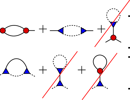
Figure 3: (Color online) Feynman diagrams of the self-energy corrections to second order in the three-legged vertices, see Eqs. (114) and (115). The slashed tadpole diagrams give frequency-independent contributions of order $1/S$ which are analytic functions of the magnetic field. Since in this work we are only interested in the frequency dependent part of the self-energy, we shall omit the tadpole diagrams.

The frequency integrations in Eqs. (114) and (115) can now be performed analytically; the relevant integrals are

$$I^{(n)}(E_{1},E_{2},\omega) = \int_{-\infty}^{\infty}\frac{dx}{2\pi}\frac{x^{n}}{[x^{2}+E_{1}^{2}][(x+\omega)^{2}+E_{2}^{2}]}$$ (116)

$$=\frac{i^{n}}{2}\left[\frac{E_{1}^{n-1}}{E_{2}^{2}-(E_{1}-i\omega)^{2}}+\frac{(E_{2}+i\omega)^{n}}{E_{2}[E_{1}^{2}-(E_{2}+i\omega)^{2}]}\right],$$

where $n=0,1,2$. Explicitly,

$$I^{(0)} = \frac{E_{1}+E_{2}}{2E_{1}E_{2}[(E_{1}+E_{2})^{2}+\omega^{2}]},$$ (117a)

$$I^{(1)} = -\frac{\omega}{2E_{2}[(E_{1}+E_{2})^{2}+\omega^{2}]},$$ (117b)

$$I^{(2)} = \frac{E_{2}(E_{1}+E_{2})+\omega^{2}}{2E_{2}[(E_{1}+E_{2})^{2}+\omega^{2}]}.$$ (117c)

The result for the self-energies can be written as

$$\Sigma_{-}(K) = \frac{h_{c}^{2}\lambda^{2}}{16S}\frac{2}{N}\sum_{\bm{q}}\left\{z_{\bm{q}+}z_{\bm{k}-\bm{q}+}\left[M_{0}^{2}(\bm{k},\bm{q})I^{(0)}_{++}(i\omega,\bm{k},\bm{q})+2M_{0}(\bm{k},\bm{q})M_{+}(\bm{k},\bm{q})I^{(1)}_{++}(i\omega,\bm{k},\bm{q})\right.\right.$$ (118)

$$\left.\hskip 108.12054pt+M^{2}_{+}(\bm{k},\bm{q})I^{(2)}_{++}(i\omega,\bm{k},\bm{q})\right]$$

$$\hskip 56.9055pt+z_{\bm{q}-}z_{\bm{k}-\bm{q}-}\left[M_{-}^{2}(\bm{k},\bm{q})I^{(0)}_{--}(i\omega,\bm{k},\bm{q})+2M_{-}(\bm{k},\bm{q})M_{-}(\bm{q},\bm{k})I^{(1)}_{--}(i\omega,\bm{k},\bm{q})\right.$$

$$\hskip 108.12054pt\left.\left.+M_{-}^{2}(\bm{q},\bm{k})I^{(2)}_{--}(i\omega,\bm{k},\bm{q})\right]\right\},$$

$$\Sigma_{+}(K) = \frac{h_{c}^{2}\lambda^{2}}{16S}\frac{2}{N}\sum_{\bm{q}}z_{\bm{q}-}z_{\bm{k}-\bm{q}+}\left[M_{+}^{2}(\bm{q},\bm{k})I^{(0)}_{-+}(i\omega,\bm{k},\bm{q})+2M_{+}(\bm{q},\bm{k})M_{0}(\bm{q},\bm{k})I^{(1)}_{-+}(i\omega,\bm{k},\bm{q})\right.$$ (119)

$$\left.\hskip 108.12054pt+M_{0}^{2}(\bm{q},\bm{k})I^{(2)}_{-+}(i\omega,\bm{k},\bm{q})\right],$$

where

$$I^{(n)}_{\sigma\sigma^{\prime}}(i\omega,\bm{k},\bm{q})=\omega^{2-n}I^{(n)}(E_{\bm{q}\sigma},E_{\bm{k}-\bm{q}\sigma^{\prime}},\omega),$$ (120)

and we have introduced the functions

$$M_{0}(\bm{k},\bm{q}) = \frac{\gamma_{\bm{q}}}{z_{\bm{k}-\bm{q}+}}-\frac{\gamma_{\bm{k}}-\gamma_{\bm{q}}-\gamma_{\bm{k}-\bm{q}}}{z_{\bm{k}-}},$$ (121a)

$$M_{+}(\bm{k},\bm{q}) = \frac{\gamma_{\bm{q}}}{z_{\bm{k}-\bm{q}+}}-\frac{\gamma_{\bm{k}-\bm{q}}}{z_{\bm{q}+}},$$ (121b)

$$M_{-}(\bm{k},\bm{q}) = \frac{\gamma_{\bm{k}}}{z_{\bm{k}-}}-\frac{\gamma_{\bm{k}-\bm{q}}}{z_{\bm{k}-\bm{q}-}}.$$ (121c)

For later reference we note that

$$M_{0}(0,\bm{q}) = \frac{\gamma_{\bm{q}}}{z_{\bm{q}+}}+\frac{2\gamma_{\bm{q}}-1}{z_{0-}},$$ (122a)

$$M_{+}(0,\bm{q}) = 0,$$ (122b)

$$M_{-}(0,\bm{q}) = \frac{1}{z_{0-}}-\frac{\gamma_{\bm{q}}}{z_{\bm{q}-}},$$ (122c)

$$M_{0}(\bm{k},0) = \frac{1}{z_{\bm{k}+}}+\frac{1}{z_{\bm{k}-}},$$ (122d)

$$M_{+}(\bm{k},0) = \frac{1}{z_{\bm{k}+}}-\frac{\gamma_{\bm{k}}}{z_{0+}},$$ (122e)

$$M_{-}(\bm{k},0) = 0.$$ (122f)

Furthermore, if both $\bm{k}$ and $\bm{q}$ are small

$$M_{-}(\bm{k},\bm{q})=\frac{a^{2}}{4Dn^{4}}\left[\bm{q}^{2}-2\bm{k}\cdot\bm{q}\right]+O(k^{4},q^{4},k^{2}q^{2}).$$ (123)

V Renormalization of the gapless magnon

V.1 Spin-wave velocity

We now show that in dimensions $D\leq 3$ the leading $1/S$-correction to the spin-wave velocity $\tilde{c}_{-}(h)$ of the gapless magnon is non-analytic in $h^{2}$. Therefore we expand for small $\omega$ and $|\bm{k}|$,

$$\Sigma_{-}(\bm{k},i\omega) = f_{0}\omega^{2}+f_{1}\omega_{\bm{k}}^{2}$$ (124)

$$+ f_{2}\omega^{4}+f_{3}\omega^{2}\omega_{\bm{k}}^{2}+f_{4}\omega_{\bm{k}}^{4}+O(\omega^{6}),$$

where $\omega$ and $\omega_{\bm{k}}=c_{-}|\bm{k}|$ are assumed to have the same order of magnitude and $c_{-}=c_{0}n^{2}$ is the spin-wave velocity within linear spin-wave theory, see Eq. (53). To calculate the renormalized spin-wave velocity we may neglect in Eq. (124) the terms of order $\omega^{4}$ involving the coefficient $f_{2}$, $f_{3}$ and $f_{4}$. Using Eqs. (112) and (113) we obtain for the infrared behavior of the propagator of the gapless mode

$$G_{-}(\bm{k},i\omega)=\frac{Z_{-}h_{c}n^{2}}{\omega^{2}+\tilde{c}_{-}^{2}\bm{k}^{2}}.$$ (125)

Introducing the dimensionless constants ${F}_{0}$ and ${F}_{1}$,

$${F}_{0}=h_{c}n^{2}f_{0},\;\;\;{F}_{1}=h_{c}n^{2}f_{1},$$ (126)

the wave-function renormalization factor $Z_{-}$ can be written as

$$Z_{-}=\frac{1}{1+{F}_{0}}\approx 1-F_{0},$$ (127)

and the renormalized spin-wave velocity $\tilde{c}_{-}$ obeys

$$\frac{\tilde{c}_{-}^{2}}{c_{-}^{2}}=\frac{1+{F}_{1}}{1+{F}_{0}}\approx 1+F_{1}-F_{0}.$$ (128)

The constants $f_{0}$ and $f_{2}$ associated with the expansion in powers of frequencies for vanishing external momentum can be obtained by expanding $\Sigma_{-}(\bm{k}=0,\omega)$ in powers of $\omega^{2}$. Using Eq. (118) and Eqs. (122a–122f) one gets

$$\Sigma_{-}(0,i\omega) = \frac{h_{c}^{2}\lambda^{2}}{16S}\frac{2}{N}\sum_{\bm{q}}\Bigl{\{}z_{\bm{q}+}^{2}M_{0}^{2}(0,\bm{q})I^{(0)}_{++}(i\omega,0,\bm{q})$$ (129)

$$\hskip 51.21495pt+z_{\bm{q}-}^{2}M_{-}^{2}(0,\bm{q})I^{(0)}_{--}(i\omega,0,\bm{q})\Bigr{\}}$$

$$= \omega^{2}\frac{h_{c}^{2}\lambda^{2}}{16S}\frac{2}{N}\sum_{\bm{q}}\biggl{\{}\frac{\bigl{[}\gamma_{\bm{q}}+\frac{1+\gamma_{\bm{q}}}{2n^{2}}(2\gamma_{\bm{q}}-1)\bigr{]}^{2}}{E_{\bm{q}+}[(2E_{\bm{q}+})^{2}+\omega^{2}]}$$

$$\hskip 42.67912pt+\frac{\bigl{[}\frac{z_{\bm{q}-}}{z_{0-}}-\gamma_{\bm{q}}\bigr{]}^{2}}{E_{\bm{q}-}[(2E_{\bm{q}-})^{2}+\omega^{2}]}\biggr{\}}.$$

Using $h_{c}^{2}\lambda^{2}=4n^{2}h^{2}$, we obtain for the first two coefficients in the frequency expansion,

$$f_{0} = \frac{n^{2}h^{2}}{16S}\frac{2}{N}\sum_{\bm{q}}\biggl{\{}\frac{\bigl{[}\gamma_{\bm{q}}+\frac{1+\gamma_{\bm{q}}}{2n^{2}}(2\gamma_{\bm{q}}-1)\bigr{]}^{2}}{E_{\bm{q}+}^{3}}$$ (130)

$$\hskip 56.9055pt+\frac{\bigl{[}\frac{z_{\bm{q}-}}{z_{0-}}-\gamma_{\bm{q}}\bigr{]}^{2}}{E_{\bm{q}-}^{3}}\biggr{\}},$$

$$f_{2} = -\frac{n^{2}h^{2}}{16S}\frac{2}{N}\sum_{\bm{q}}\biggl{\{}\frac{\bigl{[}\gamma_{\bm{q}}+\frac{1+\gamma_{\bm{q}}}{2n^{2}}(2\gamma_{\bm{q}}-1)\bigr{]}^{2}}{4E_{\bm{q}+}^{5}}$$ (131)

$$\hskip 56.9055pt+\frac{\bigl{[}\frac{z_{\bm{q}-}}{z_{0-}}-\gamma_{\bm{q}}\bigr{]}^{2}}{4E_{\bm{q}-}^{5}}\biggr{\}}.$$

Keeping in mind that $z_{\bm{q}-}/{z_{0-}}-\gamma_{\bm{q}}=O(q^{2})$ for small $q$, it is easy to see that in the domain of small magnetic field $(h\ll h_{c})$ the integrals on the right-hand sides of the equations above are dominated by the first term involving the gapped mode $E_{\bm{q}+}$. More precisely, the relevant ultraviolet cutoff for the momentum integrals in Eqs. (130, 131) is the inverse of the length scale

$$\xi=c_{0}/h.$$ (132)

In $D\leq 3$ the contribution from wave-vectors in the regime $|\bm{q}|\xi\lesssim 1$ gives rise to contributions to the magnon self-energy which are non-analytic in $h^{2}$. Keeping in mind that for small field the magnetic length $\xi$ is large compared with the lattice spacing, we may calculate the leading non-analytic magnetic-field dependent contributions to Eqs. (130, 131) by expanding the integrand in powers of $\bm{q}$.

We find that the leading magnetic field dependence of the spin-wave velocity $\tilde{c}_{-}$ associated with the gapless mode is determined by $f_{0}$. Since we are only interested in the non-analytic $h^{2}$-dependence, we may set $n\approx 1$. In the thermodynamic limit we then obtain for the dominant contribution to Eq. (130),

$$f_{0} \approx \frac{h^{2}a^{D}}{2S}\int\frac{d^{D}q}{(2\pi)^{D}}\frac{1}{E_{\bm{q}+}^{3}}.$$ (133)

Consistently neglecting terms which are analytic in $h^{2}$, we may ignore the magnetic field dependence of the non-interacting spin-wave velocities, $c_{\pm}\approx c_{0}=2\sqrt{D}JSa$, so that energy dispersions are approximated by $E_{\bm{q}-}\approx c_{0}|{\bm{q}}|$ and $E_{\bm{q}+}\approx\sqrt{h^{2}+c^{2}_{0}{\bm{q}}^{2}}$. Using $h_{c}=2\sqrt{D}c_{0}/a$ we obtain from Eq. (130) for the corresponding dimensionless coefficient for $1<D\leq 3$,

$${F}_{0}=h_{c}n^{2}f_{0}=\alpha_{D}\frac{m^{D-1}}{S},$$ (134)

where $m=h/h_{c}=ha/(2\sqrt{D}c_{0})$ is the relevant dimensionless magnetic field [see Eq. (52)], and

$$\alpha_{D}=2^{D-1}D^{D/2}K_{D}\int_{0}^{1/m}dy\frac{y^{D-1}}{[1+y^{2}]^{3/2}}.$$ (135)

Here

$$K_{D}=\frac{2^{1-D}}{\pi^{D/2}\Gamma(D/2)}$$ (136)

is the surface area of the $D$-dimensional unit sphere divided by $(2\pi)^{D}$. In $D<3$ we may take the limit $1/m\rightarrow\infty$ in $\alpha_{D}$, so that

$$\alpha_{D}=\left(\frac{D}{\pi}\right)^{D/2}\frac{\Gamma(\frac{3-D}{2})}{\sqrt{\pi}}.$$ (137)

In particular, $\alpha_{2}=2/\pi$. In $D=3$ the integral $\alpha_{3}$ depends for small $m$ logarithmically on the upper limit,

$$\alpha_{3}\sim\alpha_{3}^{\prime}\ln(1/m),\;\;\alpha_{3}^{\prime}=\frac{6\sqrt{3}}{\pi^{2}}.$$ (138)

It turns out that the coefficient $F_{1}$ in front of the $\bm{k}^{2}$-correction to the self-energy is for small $h$ proportional to $h^{2}$, so that for $h\ll\Delta$ the dominant magnetic-field dependence of the spin-wave velocity is due to the term $F_{0}$ in Eq. (128). We thus obtain for the leading magnetic field dependence of the spin-wave velocity of the gapless magnon

$$\frac{\tilde{c}_{-}^{2}}{c_{0}^{2}} \approx 1-{F}_{0}$$ (139a)

$$= 1-\frac{2}{\pi S}\frac{|\bm{h}|}{h_{c}},\;\;D=2,$$

$$= 1-\frac{6\sqrt{3}}{\pi^{2}S}\frac{\bm{h}^{2}}{h_{c}^{2}}\ln\left(\frac{h_{c}}{|\bm{h}|}\right),\;\;D=3,$$ (139b)

where we have neglected magnetic field independent $1/S$-corrections. Recall that within linear spin-wave theory the velocity $c_{-}$ of the gapless magnon is analytic in $\bm{h}^{2}=h_{c}^{2}m^{2}$; from Eq. (53) we obtain $c_{-}\approx c_{0}[1-m^{2}/2]$ for small $m$. We conclude that in dimensions $D\leq 3$ the dominant magnetic field dependence of the spin-wave velocity of the gapless magnon is due to spin-wave interactions. In Appendix B we show that the non-analytic dependence on $\bm{h}^{2}$ predicted by Eq. (139a) can be recovered numerically from in the expression for the magnon self-energy given by Zhitomirsky and Chernyshev Zhitomirsky99 .

V.2 Quasiparticle residue

In view of the fact that the magnetic field dependence of the spin-wave velocity of the gapless magnon is dominated by spin-wave interactions, it is reasonable to expect that also the higher coefficients in the expansion of the self-energy of the gapless magnon for small wave-vectors and frequencies exhibit some non-analytic dependence on the magnetic field. Consider first the renormalized magnon energies $\tilde{E}_{\bm{k}\sigma}$, which can be defined by

$$\tilde{E}_{\bm{k}\sigma}^{2}=E_{\bm{k}\sigma}^{2}+\Delta_{\bm{k}\sigma}{\rm Re}\Sigma_{\sigma}(\bm{k},\tilde{E}_{\bm{k}\sigma}+i0).$$ (140)

The expansion for small wave-vectors is

$$\tilde{E}^{2}_{\bm{k}-}=\tilde{c}_{-}^{2}\bm{k}^{2}\left[1+\tilde{A}_{-}(\hat{\bm{k}})\bm{k}^{2}+O(\bm{k}^{4})\right].$$ (141)

It is well known Landau80 that only if the coefficient $\tilde{A}_{-}$ is positive a gapless magnon with momentum $\bm{k}$ can spontaneously decay into two magnons with momenta $\bm{q}$ and ${\bm{k}}-\bm{q}$. Within linear spin-wave theory we obtain from Eqs. (40) and (45) in $D$ dimensions

$${E}^{2}_{\bm{k}-} = c_{-}^{2}\bm{k}^{2}\left[1+A_{-}(\hat{\bm{k}})\bm{k}^{2}+O(\bm{k}^{4})\right],$$ (142)

$${E}^{2}_{\bm{k}+} = h^{2}+c_{+}^{2}\bm{k}^{2}\left[1+A_{+}(\hat{\bm{k}})\bm{k}^{2}+O(\bm{k}^{4})\right],\hskip 19.91692pt$$ (143)

with

$$A_{-}(\hat{\bm{k}}) = -\frac{a^{2}}{4}\left[\frac{1-2m^{2}}{D(1-m^{2})}+\frac{1}{3}\sum_{\mu}\hat{k}_{\mu}^{4}\right],$$ (144)

$$A_{+}(\hat{\bm{k}}) = -\frac{a^{2}}{4}\left[\frac{1-2m^{2}}{D(1-3m^{2})}+\frac{1}{3}\sum_{\mu}\hat{k}_{\mu}^{4}\right].$$ (145)

Obviously, for $m\ll 1$ the coefficient $A_{-}(\hat{\bm{k}})$ is negative for all directions $\hat{\bm{k}}$, so that to this order in spin-wave theory the gapless magnon cannot spontaneously decay at long wave-lengths. For larger $m$ the coefficient $A_{-}(\hat{\bm{k}})$ decreases and eventually vanishes at a critical $m_{\ast}(\hat{\bm{k}})$ which depends on the direction $\hat{\bm{k}}$. From Eq. (144) it is easy to show that the direction where $m_{\ast}(\hat{\bm{k}})$ assumes the smallest possible value is given by the diagonal $\hat{k}_{x}=\ldots=\hat{k}_{D}$, and that the associated minimum is $m_{\ast}=h_{\ast}/h_{c}=2/\sqrt{7}\approx 0.76$. For the special case $D=2$ this result has been obtained previously by Zhitomirsky and Chernyshev Zhitomirsky99 , who examined the leading $1/S$-correction in the regime $h_{\ast}<h<h_{c}$ numerically.

Apparently, the leading $1/S$-correction in the limit of small magnetic fields $m=h/h_{c}\ll 1$ has not been explicitly analyzed in Ref. [Zhitomirsky99, ]. In terms of the expansion coefficients introduced in Eq. (124) we obtain $\tilde{A}_{-}(\hat{\bm{k}})=A_{-}(\hat{\bm{k}})+\delta A_{-}$, where the $1/S$-correction is

$$\delta A_{-}=c_{0}^{2}h_{c}\left[f_{2}-f_{3}+f_{4}\right].$$ (146)

Let us consider first the contribution from the coefficient $f_{2}$ related to the $\omega^{4}$-term in the expansion of the self-energy $\Sigma_{-}(0,i\omega)$ for small frequencies. Because for small $h$ the integral defining $f_{2}$ in Eq. (131) the dominated by wave-vectors $|\bm{q}|\lesssim h/c_{0}$, we may approximate

$$f_{2}\approx-\frac{h^{2}a^{D}}{8S}\int\frac{d^{D}q}{(2\pi)^{D}}\frac{1}{E_{\bm{q}+}^{5}}.$$ (147)

The integral is easily evaluated to leading order for small $m\ll 1$. Introducing the dimensionless coefficient

$$F_{2}\equiv\frac{c_{0}^{2}h_{c}f_{2}}{a^{2}},$$ (148)

we obtain for $D<3$,

$$F_{2}\approx-\frac{\beta_{D}}{S}\left[m^{D-3}+O(m^{D-1})\right],$$ (149)

with the numerical coefficient

$$\beta_{D} = \frac{(2\sqrt{D})^{D-2}}{8}K_{D}\int_{0}^{\infty}dx\frac{x^{D-1}}{[1+x^{2}]^{5/2}}$$ (150)

$$= \frac{(2\sqrt{D})^{D-2}}{8}K_{D}\frac{2}{3\sqrt{\pi}}\Gamma(\frac{5-D}{2})\Gamma(\frac{D}{2}).$$

In particular, in two dimensions $\beta_{2}=1/(48\pi)$. Obviously, for $D<3$ the coefficient $F_{2}$ diverges for $m\rightarrow 0$, so that the contribution from the term $f_{2}$ to $\delta A_{-}$ is for sufficiently small $m$ much larger than the linear spin-wave result (144). It turns out, however, that the singular contribution to $\delta A_{-}$ due to $f_{2}$ is exactly canceled by a similar contribution from the coefficient $f_{3}$. In order to extract the dominated contribution to $f_{3}$, it is sufficient to approximate the magnon self-energy (118) by

$$\Sigma_{-}(\bm{k},i\omega)\approx\frac{2h^{2}a^{D}}{S}\int\frac{d^{D}q}{(2\pi)^{D}}I_{++}^{(0)}(i\omega,{\bm{k}},{\bm{q}}).$$ (151)

Expanding the right-hand side to second order in $\bm{k}$ and comparing with Eq. (124), we obtain

$$f_{3} \approx -\frac{h^{2}a^{D}}{8S}\int\frac{d^{D}q}{(2\pi)^{D}}\frac{1}{E_{\bm{q}+}^{5}}\left[3-\frac{10}{D}\frac{c_{0}^{2}\bm{q}^{2}}{E_{\bm{q}+}^{2}}\right].$$ (152)

The integral can easily be carried out analytically with the result $f_{3}=f_{2}+O(m^{D-1})$. From Eq. (118) we can also show that the term $f_{4}$ is of order $a^{2}m^{D-1}/S$ and can be neglected as compared with $f_{2}$ and $f_{3}$. Because $\delta A_{-}$ involves the combination $f_{2}-f_{3}$, we conclude that the singular contributions proportional to $m^{D-3}$ cancel in $\delta A_{-}$, so that the leading magnetic field dependence of $A_{-}$ is proportional to $m^{D-1}\propto|\bm{h}|^{D-1}$. This is small compared with the linear spin-wave result but non-analytic in $\bm{h}^{2}$, similar to the leading magnetic field-dependence of the spin-wave velocity in Eqs. (139a, 139b).

On the other hand, the singular magnetic field dependence appearing in the coefficients $f_{2}$ and $f_{3}$ does not cancel in the self-energy $\Sigma_{-}(\bm{k},\omega+i0)$ off resonance. Retaining only the singular contributions to Eq. (118) we obtain with $f_{2}\approx f_{3}$

$$\Sigma_{-}(\bm{k},\omega+i0)\approx-f_{0}\omega^{2}+f_{2}\omega^{2}(\omega^{2}-\tilde{c}_{-}^{2}\bm{k}^{2}).$$ (153)

The corresponding renormalized magnon Green function for small $m$ can be written as

$$G_{-}(\bm{k},i\omega)=Z_{-}(i\omega)\frac{h_{c}n^{2}}{\omega^{2}+\tilde{c}_{-}^{2}\bm{k}^{2}},$$ (154)

where the renormalized spin-wave velocity is given in Eqs. (139a,139b), and

$$Z_{-}(i\omega) = \frac{1}{1+F_{0}+h_{c}n^{2}f_{2}\omega^{2}}$$ (155)

$$\approx 1-F_{0}-(a^{2}F_{2}/c_{0}^{2})\omega^{2}.$$

After analytic continuation to real frequencies we obtain for the renormalized residue of the magnon peak for small $m$,

$$Z_{\bm{k}-}\equiv Z_{-}(i\omega\rightarrow\tilde{c}_{-}|\bm{k}|) = 1-F_{0}+F_{2}\bm{k}^{2}a^{2}$$ (156)

$$= 1-F_{0}-\beta_{D}\frac{\bm{k}^{2}a^{2}}{Sm^{3-D}}.\hskip 28.45274pt$$

Expressing $m=h/h_{c}=ha/(2\sqrt{D}c_{0})=a/(2\sqrt{D}\xi)$ in terms of the length scale $\xi=c_{0}/h$ associated with the magnetic field we may alternatively write

$$Z_{\bm{k}-} = 1-F_{0}-\frac{\tilde{\beta}_{D}}{S}\Bigl{(}\frac{\xi}{a}\Bigr{)}^{3-D}\bm{k}^{2}a^{2}$$ (157)

$$= 1-\frac{1}{S}\Bigl{(}\frac{a}{\xi}\Bigr{)}^{D-1}\left[\tilde{\alpha}_{D}-\tilde{\beta}_{D}\bm{k}^{2}\xi^{2}\right],$$

where $\tilde{\alpha}_{D}=\alpha_{D}(2\sqrt{D})^{1-D}$ and $\tilde{\beta}_{D}=\beta_{D}(2\sqrt{D})^{3-D}$. In particular, in $D=2$ the leading momentum dependence of $Z_{\bm{k}-}$ is proportional to $\bm{k}^{2}\xi a=\bm{k}^{2}c_{0}a/h$. The higher powers in $\bm{k}$ become important for $|\bm{k}\xi|\gtrsim 1$, so that the expansion (157) is limited to the regime $|\bm{k}|\lesssim\xi^{-1}\ll a^{-1}$ where the $1/S$-correction is small compared with unity.

V.3 Magnon damping

Given the magnon self-energies $\Sigma_{\sigma}(K)$ in Eqs. (118,119) and the renormalized magnon dispersions $\tilde{E}_{\bm{k}\sigma}$, the magnon damping can be obtained from

$$\Gamma_{\bm{k}\sigma}=-\frac{\Delta_{\bm{k}\sigma}}{2\tilde{E}_{\bm{k}\sigma}}{\rm Im}\Sigma_{\sigma}(\bm{k},\tilde{E}_{\bm{k}\sigma}+i0).$$ (158)

Zhitomirsky and Chernyshev Zhitomirsky99 have shown that in two dimensions one should self-consistently take into account the imaginary part of the magnon self-energy when evaluating the integrals on the right-hand side of Eq. (118). However, as long as we are not too close to the critical field $h_{*}$, the result for the magnon damping is non-singular even if we ignore the damping of intermediate magnons in Eq. (118). We therefore expect that a simplified version of Eq. (158) taking into account only the renormalization of the real part of the magnon dispersion yields a qualitatively correct estimate for the magnon damping away from $h_{*}$.

To calculate the damping $\Gamma_{\bm{k}-}$ of the gapless magnon for wave-vectors $|\bm{k}|\ll h/c_{0}=\xi^{-1}$, it is sufficient to retain in Eq. (118) only the terms involving the functions $I^{(n)}_{--}(i\omega,\bm{k},\bm{q})$, because the imaginary part of the functions $I^{(n)}_{++}(\omega+i0,\bm{k},\bm{q})$ vanishes for $\omega<2h$. Using Eq. (123) we obtain for $\omega>0$

$${\rm Im}\left[M_{-}^{2}(\bm{k},\bm{q})I^{(0)}_{--}(\omega+i0,\bm{k},\bm{q})+2M_{-}(\bm{k},\bm{q})M_{-}(\bm{q},\bm{k})I^{(1)}_{--}(\omega+i0,\bm{k},\bm{q})+M_{-}^{2}(\bm{q},\bm{k})I^{(2)}_{--}(\omega+i0,\bm{k},\bm{q})\right]$$

$$=-\frac{\pi}{4}\left(\frac{a^{2}}{4Dn^{4}}\right)^{2}W(\bm{k},\bm{q})\delta(\omega-\tilde{E}_{\bm{k}-\bm{q}-}-\tilde{E}_{\bm{q}-}),$$ (159)

where

$$W(\bm{k},\bm{q}) = \frac{q}{|\bm{k}-\bm{q}|}(k^{2}-q^{2})^{2}+\frac{|\bm{k}-\bm{q}|}{q}(q^{2}-2\bm{k}\cdot\bm{q})^{2}$$ (160)

$$-2(k^{2}-q^{2})(q^{2}-2\bm{k}\cdot\bm{q}).$$

Note that in the non-linear sigma model the contribution corresponding to Eq. (159) is neglected because the relevant vertex involving three gapless magnons is set equal to zero (see Eq. (LABEL:eq:gammammm)), which is correct to leading order in the derivatives. Hence, the damping of the gapless magnon cannot be obtained using the NLSM. To estimate the magnon damping we set $\omega=\tilde{E}_{\bm{k}-}$ and approximate the renormalized magnon dispersion by

$$\tilde{E}_{\bm{k}-}\approx c_{-}|\bm{k}|(1+\bar{A}_{-}\bm{k}^{2}),$$ (161)

where for simplicity we have replaced the direction-dependent coefficient $\tilde{A}_{-}(\hat{\bm{k}})$ defined in Eq. (141) by some angular average $\bar{A}_{-}$. At long wave-lengths we then obtain

$$\Gamma_{\bm{k}-} = \frac{\pi\sqrt{D}}{8(4D)^{2}}\frac{h^{2}a^{D+3}}{S}\int\frac{d^{D}q}{(2\pi)^{D}}\frac{W(\bm{k},\bm{q})}{k}$$ (162)

$$\times\delta(\tilde{E}_{\bm{k}-}-\tilde{E}_{\bm{k}-\bm{q}-}-\tilde{E}_{\bm{q}-}).$$

As discussed in the textbook by Lifshitz and Pitaevskii Landau80 , in the long wave-length limit the energy conservation $\tilde{E}_{\bm{k}-}=\tilde{E}_{\bm{k}-\bm{q}-}+\tilde{E}_{\bm{q}-}$ can only be satisfied for $\bar{A}_{-}>0$. From our discussion in Sec. V.2 (see also Ref. [Zhitomirsky99, ]) we know that this condition is only satisfied in a certain range $h_{\ast}<|\bm{h}|<h_{c}$ of magnetic fields below the saturation field. We now restrict ourselves to this regime, without explicitly calculating the magnetic-field dependence of the coefficient $\bar{A}_{-}>0$. If $h$ is not very close to the threshold fields $h_{\ast}$ and $h_{c}$, we expect by dimensional analysis that $\bar{A}_{-}/a^{2}$ is a number of the order of unity. The energy conservation then implies that the allowed vectors $\bm{q}$ are almost parallel to the direction of $\bm{k}$ and satisfy $q\leq k$. In fact, it is easy to show that the angle $\vartheta$ between $\bm{k}$ and $\bm{q}$ is $\vartheta\approx\sqrt{6\bar{A}_{-}}(k-q)$ due to energy conservation so that for $\bar{A}_{-}k^{2}\ll 1$ we may approximate

$$\delta(\tilde{E}_{\bm{k}-}-\tilde{E}_{\bm{k}-\bm{q}-}-\tilde{E}_{\bm{q}-})\approx\frac{\delta(\vartheta-\sqrt{6\bar{A}_{-}}(k-q))}{\sqrt{6\bar{A}_{-}}c_{-}kq},$$ (163)

and

$$|\bm{k}-\bm{q}| \approx k-q+\frac{kq}{k-q}(1-\cos\vartheta)$$ (164)

$$\approx (k-q)(1+3\bar{A}_{-}kq).$$

Keeping in mind that $\bar{A}_{-}kq\ll 1$ we obtain from Eq. (160),

$$\frac{W(\bm{k},\bm{q})}{k}\approx 9kq(k-q).$$ (165)

The integrations in Eq. (162) are now elementary and we obtain for the damping of magnons with wave-vectors in the regime $|\bm{k}|\lesssim h/c_{0}\ll a^{-1}$ at zero temperature in $D$ dimensions,

$$\frac{\Gamma_{\bm{k}-}}{E_{\bm{k}-}}=\frac{\gamma_{D}}{S}\left(\frac{h}{h_{c}}\right)^{2}\left(\sqrt{6\bar{A}_{-}}\right)^{D-3}a^{D+1}|\bm{k}|^{2D-2},$$ (166)

where

$$\gamma_{D} = \frac{9}{64\sqrt{D}}K_{D-1}\int_{0}^{1}dx[x(1-x)]^{D-1}$$ (167)

$$= \frac{9}{64\sqrt{D}}K_{D-1}2^{1-2D}\frac{\sqrt{\pi}\Gamma(D)}{\Gamma(D+\frac{1}{2})}.$$

In two dimensions we have $\gamma_{2}=3/(128\sqrt{2}\pi)$ and

$$\Gamma_{\bm{k}-}=\frac{\gamma_{2}}{S}\left(\frac{h}{h_{c}}\right)^{2}\frac{\tilde{c}_{-}|\bm{k}|^{3}a^{3}}{\sqrt{6\bar{A}_{-}}}.$$ (168)

The $|\bm{k}|^{3}$-dependence of the magnon damping has been obtained previously by Zhitomirsky and Chernyshev Zhitomirsky99 .

VI Summary and Conclusions

The main result of this work is the discovery that in quantum Heisenberg antiferromagnets subject to a weak uniform external field the leading $1/S$-correction to the self-energy of the gapless magnon is a non-analytic function of $\bm{h}^{2}$ in dimensions $D\leq 3$. We have explicitly calculated the leading magnetic field dependence of the spin-wave velocity and the momentum-dependent quasi-particle residue of the gapless magnon. At the first sight it is surprising that for quantum antiferromagnets in a uniform magnetic field at zero temperature the dimension $D=3$ plays the role of a critical dimension below which fluctuations lead to a non-analytic magnetic field dependence of the magnon spectrum. However, the gapless magnons in our model can be viewed as an interacting Bose gas in the condensed phase Kreisel07 , where the Bogoliubov mean-field theory is known Castellani97 ; Wetterich07 to break down in dimensions $D\leq 3$.

Finally, let us point out that our hybrid approach between $1/S$-expansion and NLSM is a very convenient parameterization of the spin-wave expansion, which should also be useful in other contexts. While the calculations presented here can (with some effort) also be carried out using the conventional parameterization of the $1/S$-expansion, our hybrid approach greatly facilitates the identification of the frequency dependent contributions to the magnon self-energies which give rise to the dominant magnetic field dependent corrections to the magnon spectrum.

Appendix A Quartic spin-wave interaction in Hermitian field parameterization

In Hermitian field parameterization, the quartic part of the Hamiltonian $\hat{H}_{4}^{\prime}$ defined in Eqs. (73,74) is

$$\hat{H}^{\prime}_{4} = \frac{2}{N}\sum_{\bm{k}_{1}\bm{k}_{2}\bm{k}_{3}\bm{k}_{4}}\delta_{\bm{k}_{1}+\bm{k}_{2}+\bm{k}_{3}+\bm{k}_{4},0}$$ (A.169)

$$\times \biggl{[}\frac{1}{4!}\Bigl{(}\Gamma^{PPPP}_{++++}(\bm{k}_{1},\bm{k}_{2},\bm{k}_{3},\bm{k}_{4})\hat{P}_{\bm{k}_{1}+}\hat{P}_{\bm{k}_{2}+}\hat{P}_{\bm{k}_{3}+}\hat{P}_{\bm{k}_{4}+}+\Gamma^{PPPP}_{----}(\bm{k}_{1},\bm{k}_{2},\bm{k}_{3},\bm{k}_{4})\hat{P}_{\bm{k}_{1}-}\hat{P}_{\bm{k}_{2}-}\hat{P}_{\bm{k}_{3}-}\hat{P}_{\bm{k}_{4}-}\Bigr{)}$$

$$+\frac{1}{4!}\Bigl{(}\Gamma^{XXXX}_{----}(\bm{k}_{1},\bm{k}_{2},\bm{k}_{3},\bm{k}_{4})\hat{X}_{\bm{k}_{1}-}\hat{X}_{\bm{k}_{2}-}\hat{X}_{\bm{k}_{3}-}\hat{X}_{\bm{k}_{4}-}+\Gamma^{XXXX}_{++++}(\bm{k}_{1},\bm{k}_{2},\bm{k}_{3},\bm{k}_{4})\hat{X}_{\bm{k}_{1}+}\hat{X}_{\bm{k}_{2}+}\hat{X}_{\bm{k}_{3}+}\hat{X}_{\bm{k}_{4}+}\Bigr{)}$$

$$+\frac{1}{(2!)^{2}}\Bigl{(}\Gamma^{PPPP}_{++--}(\bm{k}_{1},\bm{k}_{2};\bm{k}_{3},\bm{k}_{4})\hat{P}_{\bm{k}_{1}+}\hat{P}_{\bm{k}_{2}+}\hat{P}_{\bm{k}_{3}-}\hat{P}_{\bm{k}_{4}-}+\Gamma^{XXXX}_{--++}(\bm{k}_{1},\bm{k}_{2};\bm{k}_{3},\bm{k}_{4})\hat{X}_{\bm{k}_{1}-}\hat{X}_{\bm{k}_{2}-}\hat{X}_{\bm{k}_{3}+}\hat{X}_{\bm{k}_{4}+}\Bigr{)}$$

$$+\frac{1}{(2!)^{2}}\Bigl{(}\Gamma^{PPXX}_{++--}(\bm{k}_{1},\bm{k}_{2};\bm{k}_{3},\bm{k}_{4})\hat{P}_{\bm{k}_{1}+}\hat{P}_{\bm{k}_{2}+}\hat{X}_{\bm{k}_{3}-}\hat{X}_{\bm{k}_{4}-}+\Gamma^{PPXX}_{--++}(\bm{k}_{1},\bm{k}_{2};\bm{k}_{3},\bm{k}_{4})\hat{P}_{\bm{k}_{1}-}\hat{P}_{\bm{k}_{2}-}\hat{X}_{\bm{k}_{3}+}\hat{X}_{\bm{k}_{4}+}\Bigr{)}$$

$$+\frac{1}{(2!)^{2}}\Bigl{(}\Gamma^{PPXX}_{++++}(\bm{k}_{1},\bm{k}_{2};\bm{k}_{3},\bm{k}_{4})\bigl{\{}\hat{P}_{\bm{k}_{1}+}\hat{P}_{\bm{k}_{2}+}\hat{X}_{\bm{k}_{3}+}\hat{X}_{\bm{k}_{4}+}\bigr{\}}+\Gamma^{PPXX}_{----}(\bm{k}_{1},\bm{k}_{2};\bm{k}_{3},\bm{k}_{4})\bigl{\{}\hat{P}_{\bm{k}_{1}-}\hat{P}_{\bm{k}_{2}-}\hat{X}_{\bm{k}_{3}-}\hat{X}_{\bm{k}_{4}-}\bigr{\}}\Bigr{)}$$

$$+\Gamma^{PXPX}_{++--}(\bm{k}_{1};\bm{k}_{2};\bm{k}_{3};\bm{k}_{4})\bigl{\{}\hat{P}_{\bm{k}_{1}+}\hat{X}_{\bm{k}_{2}+}\bigr{\}}\bigl{\{}\hat{P}_{\bm{k}_{3}-}\hat{X}_{\bm{k}_{4}-}\bigr{\}}\biggr{]},$$

where the symmetrization symbol $\{\ldots\}$ is defined in Eq. (67) and we have used

$$\bigl{\{}\hat{P}_{1}\hat{P}_{2}\hat{X}_{3}\hat{X}_{4}\bigr{\}} = \frac{1}{2}\left[\hat{P}_{1}\hat{P}_{2},\hat{X}_{3}\hat{X}_{4}\right]_{+}+\frac{1}{4}\left(\delta_{1+3,0}\delta_{2+4,0}+\delta_{1+4,0}\delta_{2+3,0}\right).\hskip 19.91692pt$$ (A.170)

For convenience we now introduce the short notation $\gamma_{\bm{k}_{1}}\equiv\gamma_{\bm{1}}$, $\gamma_{\bm{k}_{2}}\equiv\gamma_{\bm{2}}$ (and similarly for the other labels) and symmetrize the vertices whenever the interaction is symmetric with respect to the exchange of the field labels. For the vertices involving four fields of the same type we obtain

$$\Gamma^{XXXX}_{----}(\bm{k}_{1},\bm{k}_{2},\bm{k}_{3},\bm{k}_{4}) = \frac{h_{c}}{16S}\Big{[}\gamma_{\bm{1}}+\gamma_{\bm{2}}+\gamma_{\bm{3}}+\gamma_{\bm{4}}-2\alpha(\gamma_{\bm{1}+\bm{2}}+\gamma_{\bm{3}+\bm{4}})+(\bm{2}\leftrightarrow\bm{3})+(\bm{2}\leftrightarrow\bm{4})\Bigr{]},$$

$$\Gamma^{XXXX}_{++++}(\bm{k}_{1},\bm{k}_{2},\bm{k}_{3},\bm{k}_{4}) = \frac{h_{c}}{16S}\Bigl{[}\alpha(\gamma_{\bm{1}}+\gamma_{\bm{2}}+\gamma_{\bm{3}}+\gamma_{\bm{4}})-2\alpha(\gamma_{\bm{1}+\bm{2}}+\gamma_{\bm{3}+\bm{4}})+(\bm{2}\leftrightarrow\bm{3})+(\bm{2}\leftrightarrow\bm{4})\Bigr{]},$$

$$\Gamma^{PPPP}_{++++}(\bm{k}_{1},\bm{k}_{2};\bm{k}_{3},\bm{k}_{4}) = \frac{h_{c}}{16S}\Bigl{[}-\gamma_{\bm{1}}-\gamma_{\bm{2}}-\gamma_{\bm{3}}-\gamma_{\bm{4}}-2\alpha(\gamma_{\bm{1}+\bm{2}}+\gamma_{\bm{3}+\bm{4}})+(\bm{2}\leftrightarrow\bm{3})+(\bm{2}\leftrightarrow\bm{4})\Bigr{]},$$

$$\Gamma^{PPPP}_{----}(\bm{k}_{1},\bm{k}_{2},\bm{k}_{3},\bm{k}_{4}) = \frac{h_{c}}{16S}\Bigl{[}-\alpha(\gamma_{\bm{1}}+\gamma_{\bm{2}}+\gamma_{\bm{3}}+\gamma_{\bm{4}})-2\alpha(\gamma_{\bm{1}+\bm{2}}+\gamma_{\bm{3}+\bm{4}})+(\bm{2}\leftrightarrow\bm{3})+(\bm{2}\leftrightarrow\bm{4})\Bigr{]}.$$

The vertices involving two pairs of fields of the same type can be written as

$$\Gamma^{XXXX}_{--++}(\bm{k}_{1},\bm{k}_{2};\bm{k}_{3},\bm{k}_{4}) = \frac{h_{c}}{16S}\Bigl{[}\gamma_{\bm{1}}+\gamma_{\bm{2}}+\alpha(\gamma_{\bm{3}}+\gamma_{\bm{4}})-2\alpha(\gamma_{\bm{1}+\bm{2}}+\gamma_{\bm{3}+\bm{4}})\Bigr{]},$$ (A.175)

$$\Gamma^{PPPP}_{++--}(\bm{k}_{1},\bm{k}_{2};\bm{k}_{3},\bm{k}_{4}) = \frac{h_{c}}{16S}\Bigl{[}-\gamma_{\bm{1}}-\gamma_{\bm{2}}-\alpha(\gamma_{\bm{3}}+\gamma_{\bm{4}})-2\alpha(\gamma_{\bm{1}+\bm{2}}+\gamma_{\bm{3}+\bm{4}})\Bigr{]},$$ (A.176)

$$\Gamma^{PPXX}_{++--}(\bm{k}_{1},\bm{k}_{2};\bm{k}_{3},\bm{k}_{4}) = \frac{h_{c}}{16S}\Bigl{[}3(-\gamma_{\bm{1}}-\gamma_{\bm{2}}+\gamma_{\bm{3}}+\gamma_{\bm{4}})$$ (A.177)

$$\hskip 22.76219pt-2\alpha\left(\gamma_{\bm{1}+\bm{2}}+\gamma_{\bm{3}+\bm{4}}-\gamma_{\bm{1}+\bm{3}}-\gamma_{\bm{2}+\bm{4}}-\gamma_{\bm{2}+\bm{3}}-\gamma_{\bm{1}+\bm{4}}\right)\Bigr{]},$$

$$\Gamma^{PPXX}_{--++}(\bm{k}_{1},\bm{k}_{2};\bm{k}_{3},\bm{k}_{4}) = \frac{h_{c}}{16S}\Bigl{[}3\alpha(-\gamma_{\bm{1}}-\gamma_{\bm{2}}+\gamma_{\bm{3}}+\gamma_{\bm{4}})$$ (A.178)

$$\hskip 22.76219pt-2\alpha\left(\gamma_{\bm{1}+\bm{2}}+\gamma_{\bm{3}+\bm{4}}-\gamma_{\bm{1}+\bm{3}}-\gamma_{\bm{2}+\bm{4}}-\gamma_{\bm{2}+\bm{3}}-\gamma_{\bm{1}+\bm{4}}\right)\Bigr{]},\hskip 28.45274pt$$

$$\Gamma^{PPXX}_{++++}(\bm{k}_{1},\bm{k}_{2};\bm{k}_{3},\bm{k}_{4}) = \frac{h_{c}}{16S}\Bigl{[}-\gamma_{\bm{1}}-\gamma_{\bm{2}}+\alpha(\gamma_{\bm{3}}+\gamma_{\bm{4}})-2\alpha(\gamma_{\bm{1}+\bm{2}}+\gamma_{\bm{3}+\bm{4}})\Bigr{]},$$ (A.179)

$$\Gamma^{PPXX}_{----}(\bm{k}_{1},\bm{k}_{2};\bm{k}_{3},\bm{k}_{4}) = \frac{h_{c}}{16S}\Bigl{[}-\alpha(\gamma_{\bm{1}}+\gamma_{\bm{2}})+\gamma_{\bm{3}}+\gamma_{\bm{4}}-2\alpha(\gamma_{\bm{1}+\bm{2}}+\gamma_{\bm{3}+\bm{4}})\Bigr{]}.$$ (A.180)

And finally, there is one vertex without permutation symmetry connecting four different field types footnoteminus ,

$$\Gamma^{PXPX}_{++--}(\bm{k}_{1};\bm{k}_{2};\bm{k}_{3};\bm{k}_{4}) = \frac{h_{c}}{16S}\Bigl{[}\gamma_{\bm{1}}+\alpha(-\gamma_{\bm{2}}+\gamma_{\bm{3}})-\gamma_{\bm{4}}-2\alpha(\gamma_{\bm{1}+\bm{4}}+\gamma_{\bm{2}+\bm{3}})\Bigr{]}.$$ (A.181)

Note that the above vertices are analytic functions of the external momenta and of $h^{2}$. On the other hand, if we express $\hat{H}_{4}^{\prime}$ in terms of the usual magnon creation and annihilation operators, we obtain vertices which are singular for certain combinations of external momenta Harris71 ; Kopietz90 ; Hasselmann07 .

Appendix B Numerical confirmation of Equation (139a) in two dimensions

In this appendix we briefly review the calculation of the $1/S$-corrections to the field dependent spin-wave dispersion in two dimensions as obtained within the conventional $1/S$-expansion by Zhitomirsky and Chernyshev in Ref. [Zhitomirsky99, ]. From the numerical analysis of this expression we quantitatively confirm our result given in Eq. (139a) for the linear magnetic field dependence of the spin-wave velocity associated with the gapless magnon. In our notation the expression for the on-shell renormalized magnon energy $\tilde{E}_{\bm{k}\sigma}$ given in Ref. [Zhitomirsky99, ] can be written as

$$\tilde{E}_{\bm{k}\sigma}=E_{\bm{k}\sigma}+\textrm{Re }\Sigma^{1/S}_{\sigma}(\bm{k},E_{\bm{k}\sigma}+i0)\,,$$ (B.182)

where the self-energy has the form

$$\Sigma^{1/S}_{\sigma}(\bm{k},i\omega) = \Sigma^{1/S}_{1\sigma}(\bm{k},i\omega)+\Sigma^{1/S}_{2\sigma}(\bm{k},i\omega)$$ (B.183)

$$+\Sigma^{1/S}_{3\sigma}(\bm{k})+\Sigma^{1/S}_{4\sigma}(\bm{k})\,.$$

The frequency dependent contributions to the self-energy are given by

$$\Sigma^{1/S}_{1\sigma}(\bm{k},i\omega)=\frac{h_{c}^{2}\lambda^{2}}{16S}\frac{2}{N}\sum_{\bm{q}\tau}\frac{\Phi_{1}^{2}(\bm{k}\sigma,\bm{q}\tau,\bm{k}-\bm{q}\overline{\sigma\tau})}{i\omega-E_{\bm{q}\tau}-E_{\bm{k}-\bm{q}\overline{\sigma\tau}}}\,,$$ (B.184)

$$\Sigma^{1/S}_{2\sigma}(\bm{k},i\omega)=-\frac{h_{c}^{2}\lambda^{2}}{16S}\frac{2}{N}\sum_{\bm{q}\tau}\frac{\Phi_{2}^{2}(\bm{k}\sigma,\bm{q}\tau,\bm{k}+\bm{q}\overline{\sigma\tau})}{i\omega+E_{\bm{q}\tau}+E_{\bm{k}+\bm{q}\overline{\sigma\tau}}}\,,$$ (B.185)

where $\overline{\sigma}=-\sigma$ denotes a sign change such that $\overline{\sigma\tau}=-\sigma\tau$, and the functions $\Phi_{1}$ and $\Phi_{2}$ are defined as

$$\Phi_{1}(\bm{k}_{1}\sigma_{1},\bm{k}_{2}\sigma_{2},\bm{k}_{3}\sigma_{3}) = \sigma_{1}\gamma_{\bm{1}}(u_{\bm{1}\sigma_{1}}+\sigma_{1}v_{\bm{1}\sigma_{1}})(\sigma_{3}u_{\bm{2}\sigma_{2}}v_{\bm{3}\sigma_{3}}+\sigma_{2}u_{\bm{3}\sigma_{3}}v_{\bm{2}\sigma_{2}})$$ (B.186)

$$+ \sigma_{2}\gamma_{\bm{2}}(u_{\bm{2}\sigma_{2}}+\sigma_{2}v_{\bm{2}\sigma_{2}})(u_{\bm{1}\sigma_{1}}u_{\bm{3}\sigma_{3}}+\sigma_{3}\sigma_{1}v_{\bm{3}\sigma_{3}}v_{\bm{1}\sigma_{1}})$$

$$+ \sigma_{3}\gamma_{\bm{3}}(u_{\bm{3}\sigma_{3}}+\sigma_{3}v_{\bm{3}\sigma_{3}})(u_{\bm{2}\sigma_{2}}u_{\bm{1}\sigma_{1}}+\sigma_{1}\sigma_{2}v_{\bm{1}\sigma_{1}}v_{\bm{2}\sigma_{2}})\,,$$

$$\Phi_{2}(\bm{k}_{1}\sigma_{1},\bm{k}_{2}\sigma_{2},\bm{k}_{3}\sigma_{3}) = \sigma_{1}\gamma_{\bm{1}}(u_{\bm{1}\sigma_{1}}+\sigma_{1}v_{\bm{1}\sigma_{1}})(\sigma_{2}u_{\bm{3}\sigma_{3}}v_{\bm{2}\sigma_{2}}+\sigma_{3}u_{\bm{2}\sigma_{2}}v_{\bm{3}\sigma_{3}})$$ (B.187)

$$+ \sigma_{2}\gamma_{\bm{2}}(u_{\bm{2}\sigma_{2}}+\sigma_{2}v_{\bm{2}\sigma_{2}})(\sigma_{1}u_{\bm{3}\sigma_{3}}v_{\bm{1}\sigma_{1}}+\sigma_{3}u_{\bm{1}\sigma_{1}}v_{\bm{3}\sigma_{3}})$$

$$+ \sigma_{3}\gamma_{\bm{3}}(u_{\bm{3}\sigma_{3}}+\sigma_{3}v_{\bm{3}\sigma_{3}})(\sigma_{1}u_{\bm{2}\sigma_{2}}v_{\bm{1}\sigma_{1}}+\sigma_{2}u_{\bm{1}\sigma_{1}}v_{\bm{2}\sigma_{2}})\,.$$

The frequency independent $1/S$-contributions to the self-energy are

$$\Sigma^{1/S}_{3\sigma}(\bm{k}) = \frac{h_{c}}{2S}(u_{\bm{k}\sigma}^{2}+v_{\bm{k}\sigma}^{2})[-\kappa_{1}\alpha+\kappa_{2}n^{2}-\kappa_{3}m^{2}+\sigma\gamma_{\bm{k}}(-\kappa_{3}\alpha+\kappa_{4}n^{2}/2-\kappa_{1}m^{2})]$$ (B.188)

$$- \frac{h_{c}}{2S}\sigma u_{\bm{k\sigma}}v_{\bm{k\sigma}}[\kappa_{2}m^{2}-\kappa_{3}n^{2}+2\sigma\gamma_{\bm{k}}(\kappa_{2}\alpha-\kappa_{1}n^{2}+\kappa_{4}m^{2}/2)]\,,$$

$$\Sigma^{1/S}_{4\sigma}(\bm{k}) = \frac{h_{c}}{S}m^{2}(\kappa_{2}-\kappa_{1}+\kappa_{3})[(u_{\bm{k}\sigma}^{2}+v_{\bm{k}\sigma}^{2})(1-\sigma\gamma_{\bm{k}})-2\gamma_{\bm{k}}u_{\bm{k}\sigma}v_{\bm{k}\sigma}]\,,$$ (B.189)

Figure 4: Evolution of the spin-wave velocity of the gapless magnon as a function of the external magnetic field for $S=1/2$. The full line shows the spin-wave velocity obtained numerically from Eq. (B.182) normalized by the zero-field value $\tilde{c}_{0}\approx 1.16c_{0}$ for $S=1/2$ (see Ref. [Oguchi60, ])). The dashed line shows the prediction of Eq. (139a). Good agreement is obtained in the limit of vanishing fields which confirms that the leading field dependence is described by Eq. (139a).

with

$$\kappa_{1} = \frac{2}{N}\sum_{\bm{k}\sigma}v_{\bm{k}\sigma}^{2}\,,$$ (B.190a)

$$\kappa_{2} = \frac{2}{N}\sum_{\bm{k}\sigma}v_{\bm{k}\sigma}u_{\bm{k}\sigma}\gamma_{\bm{k}}\,,$$ (B.190b)

$$\kappa_{3} = \frac{2}{N}\sum_{\bm{k}\sigma}\sigma v_{\bm{k}\sigma}^{2}\gamma_{\bm{k}}\,,$$ (B.190c)

$$\kappa_{4} = \frac{2}{N}\sum_{\bm{k}\sigma}\sigma v_{\bm{k}\sigma}u_{\bm{k}\sigma}\,.$$ (B.190d)

While the self-energy (B.183) can be easily evaluated numerically, it is not very accessible for analytical treatments and the leading small field behavior of the spin-wave dispersion is not easily extracted from it. The equivalent expression Eq. (118) in the Hermitian field parametrization is more amenable to an analytical investigation of the long wavelength physics. To calculate the self-energy given in Eq. (B.183) we performed a two dimensional integration and used an analytical continuation to real frequencies. Performing a numerical derivative with respect to the momentum $\bm{k}$ at the point in the Brillouin zone where the dispersion is gapless finally yields the spin-wave velocity. In Fig. 4 we compare the numerically obtained spin-wave velocity of the gapless mode at small fields with the prediction of Eq. (139a). At very small fields, the numerical solution indeed confirms the behavior given in Eq. (139a). For slightly larger fields, corrections beyond the linear dependence are also visible.

References

- (1) T. Holstein and H. Primakoff, Phys. Rev. 58, 1098 (1940).
- (2) F. J. Dyson, Phys. Rev. 102, 1217 and 1230 (1956).
- (3) S. V. Maleyev, Zh. Eksp. Teor. Fiz. 30, 1010 (1957) [Sov. Phys. JETP 64, 654 (1958)].
- (4) T. Oguchi, Phys. Rev. 117, 117 (1960).
- (5) A. B. Harris, D. Kumar, B. I. Halperin, and P. C. Hohenberg, Phys. Rev. B 3, 961 (1971).
- (6) P. Kopietz, Phys. Rev. B 41, 9228 (1990).
- (7) N. Hasselmann and P. Kopietz, Europhys. Lett. 74, 1067 (2006).
- (8) S. V. Maleyev, Phys. Rev. Lett. 85, 3281 (2000).
- (9) S. Chakravarty, B. I. Halperin, and D. R. Nelson, Phys. Rev. B 39, 2344 (1989).
- (10) M. E. Zhitomirsky and A. L. Chernyshev, Phys. Rev. Lett. 82, 4536 (1999).
- (11) A. V. Syromyatnikov and S. V. Maleyev, Phys. Rev. B 65, 012401 (2001).
- (12) D. S. Fisher, Phys. Rev. B 39, 11783 (1989).
- (13) S. Sachdev, Quantum Phase Transitions, (Cambridge University Press, Cambridge, 1999).
- (14) F. Schütz, M. Kollar, and P. Kopietz, Phys. Rev. Lett. 91, 017205 (2003).
- (15) I. Spremo, F. Schütz, P. Kopietz, V. Pashchenko, B. Wolf, M. Lang, J. W. Bats, C. Hu, and M. U. Schmidt, Phys. Rev. B 72, 174429 (2005).
- (16) N. Hasselmann, F. Schütz, I. Spremo, and P. Kopietz, C. R. Chimie 10, 60 (2007).
- (17) P. W. Anderson, Phys. Rev. 86, 694 (1952).
- (18) L. S. Schulman, Techniques and Applications of Path Integration, (Wiley, New York, 1981).
- (19) J. W. Negele and H. Orland, Quantum Many-Particle Systems, (Addison-Wesley, Redwood City, 1988).
- (20) T. Gollisch and C. Wetterich, Phys. Rev. Lett. 86, 1 (2001); M. Weyrauch and A. W. Schreiber, Phys. Rev. Lett. 88, 078901 (2002).
- (21) M. E. Zhitomirsky and T. Nikuni, Phys. Rev. B 57, 5013 (1998).
- (22) E. M. Lifshitz and and L. P. Pitaevskii, Statistical Physics II, (Pergamon, Oxford, 1980).
- (23) A. Kreisel, N. Hasselmann, and P. Kopietz, Phys. Rev. Lett. 98, 067203 (2007).
- (24) C. Castellani, C. Di Castro, F. Pistolesi, and G. C. Strinati, Phys. Rev. Lett. 78, 1612 (1997); F. Pistolesi, C. Castellani, C. Di Castro, and G. C. Strinati, Phys. Rev. B 69, 024513 (2004).
- (25) C. Wetterich, arXiv:0712.1926v1.
- (26) There is a mistake in Eq. (13e) of Ref. [Hasselmann06, ]: the term should be multiplied by a factor of . Taking into account the different labeling of the fields in Ref. [Hasselmann06, ] as compared with the labeling in Eq. (A.169) [so that we should rename ], in the limit of vanishing magnetic field the vertices in Eqs. (LABEL:eq:Gamma4_1–A.181) are then equivalent to the vertices given in Ref. [Hasselmann06, ].