Improved method of the Extensive Air Shower
arrival direction estimation

Abstract

The properties of measuring systems of the Extensive Air Showers arrival directions (EAS goniometers), consisting of some sets of widely separated detectors registering the moments of EAS frontal passage, are considered. The advantage of volumetric goniometers in comparison with the commonly used flat ones is shown. The proper points selection method for detectors spatial arranging is suggested, providing the best accessible accuracy of the EAS arrival direction estimation within the given detectors’ number and installation overall dimensions.

1 Introduction

Since the discovery of cosmic rays (CR) the problem of large-scale correlations has been almost disregarded. This is because charged particles, composing a main part of CR, must be deflected in the galactic magnetic field throughout their long journeys to the Earth, resulting in random injections into atmosphere of CR particle pairs, coinciding both in time and in direction. However, there exist some processes, engendering such pairs and groups of correlated primary particles in cosmic radiation. There may be, e.g., groups from the $\gamma$-bursts, the product $\gamma$-rays from super high energy collisions in the interstellar substance (especially in the immediate vicinity of CR generation areas), or the products of CR nuclei disintegration in the solar photon field – i.e. the effect presented by Gerasimova and Zatsepin [1, 2], etc.

All this effects are very rare, but during the last years there appeared some observational evidence of their existence [3, 4, 5] . All of them were performed by observation of correlated Extensive Air Showers (EAS). Actually, only both the registration times’ coincidence and the coincidence of two EAS cores’ directions with account of spatial positions of registration points on the Earth’s surface, can state as a partial warranty of their genetic relationship

The problem can be solved in principle by the pool of modern complicated installations, investigating the $\gamma$-initiated EAS, such as the MAGIC in the Canary Islands [6] or VERITAS in southern Arizona [7]. These installations detect and log out the showers by observation of Cherenkov light generated in the atmosphere by the quick charged particles composing the EAS. The arrival direction measurement precision of $0.15^{\circ}$ is expected [8] for individual $\gamma$-quanta.

However, these extremely perfect installations are rarely disposed on the Globe. The active observation time is limited by the atmosphere state condition. The viewing angle usually is moderate, e.g. the VERITAS array [8] observes concurrently the sky area of $3.5^{\circ}$ only. Thus it is not expectable for these expensive installations to constitute some effective pool for uninterrupted monitoring of rare events of widely spaced genetically related showers.

It is safe to say that the widespread network of small traditional ground-based installations, recording both the EAS event absolute astronomical time (UT) and the shower arrival direction on the local upper hemisphere (and measuring the EAS energy too, if possible), would make up more suitable tool for the problem. The installations of this type, being comparatively simple and inexpensive, would form reasonable equipment for university teems and research groups round the Globe, constituting the synchronized united network.

Now, as a matter of notational convenience, let us term any ground-based installation, intended for the EAS arrival direction measurement, as EAS goniometer.

The LAAS group [9] has performed   the network observation   of EAS   with energy $(10^{13}\div 10^{16})eV$, using ten independent scintillator goniometers arranged over a very large area. Especially this last group has investigated the EAS pairs coincidence not only by the times registered (using the Global Positioning System GPS) at the network stations, but also by the EAS arrival directions coincidence. This group has declared the attained measurement accuracy of EAS arrival direction to be about $10^{\circ}$ for the zenith angles less then $45^{\circ}$. This attainment is too small for the reliable paternal affiliation in the pairs observed. The analysis of the typical station construction of the network [9] gives the opportunity to ascertain the possibility of much greater angular accuracy achievement even with the same number of detectors as in the EAS goniometer used there. It becomes possible to get an acceptable accuracy even for big zenith angles. This accuracy growth is very important for any network of remote stations as far as the potentially correlated showers prove to be close to the horizon for big enough angular distances between the stations. Just for the last cases the extensively used flat EAS goniometers with poor accuracy at large zenith angles are especially objectionable.

2 Volumetric EAS goniometer. Common case.

Generally the set of any $N_{0}$ ionizing radiation detectors, arbitrarily distributed in the 3–space, can be used as the volumetric EAS goniometer. Some “triggering structure” for EAS discovering is implied. This structure has to send a trigger signal to the measuring part of installation to start a time reckoning of the pulses from EAS goniometer detectors. In particular, the EAS goniometer detectors themselves can be used for this purpose. The signals from all detectors have to be delayed for the common period, $t_{del}$, with respect to the real moments of the pulses origins. This delay period has to be such that at any possible case of the shower arrival direction all $N_{0}$ detector signals would hit the measuring part of installation later then the trigger signal. The measuring part itself records the differences of signal arrival times with respect to the trigger signal hit time as well as the absolute astronomic time (UT) of trigger signal obtained by means of GPS. Only this set of recorded numbers has to be used later (off line) to estimate the direction and the shower front passing time through the installation’s coordinate system origin.

Hereinafter all delay periods are measured in distance unites , that is to say their clock estimations are multiplied in advance by the EAS front velocity, which is taken to be approximately equal to the light velocity.

Let us fix the rectangular coordinate system for the volumetric EAS goniometer. All coordinates, times, their differences and distances are referred hereinafter to the mentioned coordinate system and are measured in meters. Furthermore, let us designate the coordinates of used detector centers as

$$\textbf{r}_{i}(x,y,z)\quad i=1,2,3\ldots N_{0}$$

The EAS front plane equation [10] at arbitrary moment is

$$\textbf{r}\cdot\textbf{n}-p=0$$ (1)

Here r is an arbitrary point in the front plane; vector n is the main unit ort of the plane, $\textbf{n}^{2}=1$, while the $p$ parameter measures the distance between the plane and coordinate system origin. Our aim is to estimate the ort components by the measured times of the front passage through the detectors.

The distances from the detectors to the front plane in any position, specified by $p$ parameter value, is determined by the linear relationship

$$\delta_{i}=\textbf{r}\cdot\textbf{n}-p\quad i=1,2,3\ldots N_{0}$$ (2)

Let us select from the whole family of planes, corresponding to the different moments of the shower propagation, the unique plane containing the coordinate origin. The last restriction implies the selection of the special plane from the planes’ family (1), singled out by the condition $p=0$ . Just this plane will be referred as “the EAS front plane”.

For this unique EAS front plane the set (2) of detectors’ distances from the front plane are

$$\delta_{i}=\textbf{r}\cdot\textbf{n}$$ (3)

There can be some negative distances between them in common case, as any of the detector points $\textbf{r}_{i}$ can be disposed on any side the EAS front plane. That is why we shall add an artificial and big enough common delay period $t_{del}$ to both sides of equation (3) (for instance, this delay can be attained by use of coupling cables with identical and big enough lengths):

$$\textbf{r}\cdot\textbf{n}+t_{del}=\delta_{i}+t_{del}\doteq t_{tr}+t_{i}$$ (4)

Here $t_{i}$ values are the measured by the EAS goniometer installation delay periods of detectors’ signals with respect to trigger signal (all of them are the positive values), while $t_{tr}$ is the (unknown) triggering time.

The decision variables in equation (4) are: the common difference of delay period of the moment when the EAS front plane passes the coordinate system origin of the installation with the triggering time, $t_{\delta}=t_{del}-t_{tr}$, and three nondimensional components of main ort n, i.e. the directional cosines of EAS core. The common difference period $t_{\delta}$ permits to obtain the UT of EAS front plane pass through the coordinate system origin (with use of the GPS–measured triggering time and common signal delay period known). Since there are 4 decision variables, so the requirement on the detectors number $N_{0}\geq 4$ is the solvability condition of equation (4). It is possible to get the solution even for three detectors, but it proves to be the singular case of system (4), demanding a special solution method. This case of “flat” EAS goniometer is considered later. Hereon the common case is studied.

For the case of detector number $N_{0}>4$ the EAS goniometer equations system

$$\textbf{r}\cdot\textbf{n}+t_{\delta}=t_{i}$$ (5)

is overfilled. The Least-Squares Method (LSM) [11, 13] is to be used to determine the solution.

It is convenient to define new vector ${\nu}$ with 4 rows for the generalized main ort of the shower front plane, with the nondimensional $4^{th}$ component ${\nu}_{t}$ to measure the value of desired common delay difference. The coordinates of all used detectors constitute the $4\times N_{0}$ matrix ${\rho}$ with dummy $4^{th}$ column, containing identical $4^{th}$ component value $\lambda=1m$ for all detectors. The measured delay periods constitute the $N_{0}$-row vector ${\tau}$. Now the equation (5) takes the form of common matrix one:

$$\rho\nu=\tau$$ (6)

As usual [11, 13] for the overfilled equation set in the frames of LSM, for delay periods distributed with dispersion matrix ${\Sigma}$, let us apply the left multiplication by $({\rho}^{T}\Sigma^{-1})$ matrix to the equation (6). This results in normal equations set for the 4 decision components of the generalized direction ort of the EAS front plane

$$A\nu=d$$ (7)

with the symmetric $4\times 4$ square matrix

$$A={\rho}^{T}\Sigma^{-1}{\rho}$$ (8)

and new right-hand member of equation

$$d={\rho}^{T}\Sigma^{-1}{\tau}$$ (9)

It has the unique solution for the nonsingular matrix ${A}$. Just due to (8) it becomes necessary to arrange the detectors set in full 3D space, not in any plane in it. The explicit solution is

$$\nu=A^{-1}d$$ (10)

or, directly expressed by the delay vector $\tau$

$$\nu=G\tau$$ (11)

Here ${G}$ is the $N_{0}\times 4$ matrix

$$G=A^{-1}\rho^{T}\Sigma^{-1}=(\rho^{T}\Sigma^{-1}\rho)^{-1}\rho^{T}\Sigma^{-1}$$ (12)

The estimation (11) of the generalized main ort evaluated here is consistent, unbiased and asymptotically normal estimator (i.e. the expectation value of the estimator coincides with the true value of the ort), as it is received from the initial data by means of the linear Least Squares Method[12].

Essentially, expression (11) is the whole solution in the common case, but the error analysis for this solution gives one the possibility to recognize some additional location requirements for the final achievement of desired estimation quality of EAS direction.

At this stage let us assume the coordinates of detectors to be taken as exactly prescribed. Practically it means that the detectors’ location errors have to be less then the errors of delay periods at least by an order of magnitude.

The generalized direction ort, ${\nu}$, is linearly connected with the measured delay periods by (11). So the dispersion matrix, ${D}$ (of the direction ort ${\nu}$), is connected with the delay dispersion matrix, ${\Sigma}$, by the linear transformation [13], too:

$$D=G\Sigma G^{T}$$ (13)

At this stage let us assume as a hypothesis that all delay periods, $t_{i}$, are identically distributed independent quantities with the same dispersion values, ${\sigma}^{2}$. This assumption is very close to reality, indeed, as the processes in one delay device do not affect the properties of another one. Hence, there are no correlations in the dispersion matrix ${\Sigma}$ of the delay vector $\tau$. On the other hand, all delay errors in every signal path originate from the similar reasons, so they can be considered as equal on average. Therefore we can accept the relation

$$\Sigma=\sigma^{2}I$$ (14)

Here ${{I}}$ is the $4\times 4$ unity matrix.

In this special case the dispersion matrix of the required vector ${\nu}$ can be expressed in explicit form via the ${{A}}$ matrix (7):

$$D=A^{-1}$$ (15)

So, all volumetric EAS goniometer properties are determined through the detectors arranging matrix ${\rho}$ and delay dispersion value ${\sigma}^{2}$ (see (8)(14)).

Broadly speaking, it is commonly desirable for the sought quantities (i.e. the generalized direction ort ${\nu}$ components in our case) to be statistically uncorrelated estimators at least. It is desired for the component dispersions to be equal, too. These requirements are strong enough. They will give us the possibility to define more accurately the best scheme of detectors arranging in the space.

3 Multitier EAS goniometer

  If it is planed to place the EAS goniometer on the flat horizontal plain, the local vertical line becomes the preferential direction in the space and it is natural to orientate the installation upon the last one. It is clear that the error isotropy of EAS direction estimations for the upper hemisphere is desired.

  Let us consider a multitier scheme of volumetric EAS goniometer. It consists of $N_{0}$ detectors arranged on several horizontal plane levels (tiers). Such a construction prevents the possible singularity of equation (7). It is clear that the desirable azimuth symmetry of errors results in axial symmetry of detectors position on every tier. In the simplest case ( see Fig.1) they are placed uniformly along the circumferences with centers based on a common vertical axis.

  All detectors hereon belong to the goniometer subsystem itself, the trigger subsystem is not considered.

Let us use the rectangular frame of reference with horizontal $XOY$ plane and with $OZ$ axes directed upwards along the local vertical line. Axes $OX$ is a polar one for the azimuth angles.

All detectors are situated on $M$ horizontal levels; $\quad a=1,2,3\ldots M\quad$ are indexes of these levels.

Every $a$–level contains $N_{a}$ detectors. The total number of detectors is

$$N_{0}=\sum_{a=1}^{M}N_{a}$$ (16)

The radii of the detectors’ positions regarding to the $OZ$ axis are $R_{a}$ at any a–level, while $H_{a}$ are the levels’ heights above the $XOY$ plane.

At any $a$–level a separate detectors numeration is established: $k=1,2,3,\ldots N_{a}\quad$ are the indexes of detectors at each level.

These detectors divide uniformly corresponding circle of $R_{a}$ radius with the angular step

$$\alpha_{a}=\frac{2\pi}{N_{a}}$$ (17)

Detectors are represented by points in the polygon apexes at any level. The detector numbers for the example shown are:

$$N_{1}=8;\;N_{2}=8;\;\ldots N_{M}=4.$$

The planes of tiers are displayed conditionally for visual manifestation of axial symmetry only.

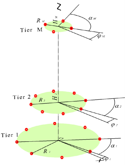
Figure 1: The detectors’ position scheme for the multitier EAS goniometer.

The phase shifts of detectors situated along the $a$–level circumferences are denoted as $\varphi_{a}$. Every delay period $t_{a,k}$ of detector with item number $k$, disposed on the $a$–level, has to be recorded as a result of installation triggering due to EAS front passage through the EAS goniometer.

It is clear that the $a$–level detectors are situated in the points with the coordinates:

$$(X_{a,k}=R_{a}\cos(k\alpha_{a}+\varphi_{a}),\;Y_{a,k}=R_{a}\sin(k\alpha_{a}+\varphi_{a}),\;H_{a},\;\lambda)$$ (18)

— just these sets of coordinates constitute the $N_{0}$- -row matrix $\rho$ of detectors’ positions.

The circles division mode used above provides the definitive calculation [14] of the $A$ matrix (8) in the explicit form.

It is convenient to define the “tier averaging” operation for any set of values $Q_{a}$ representing some property of every level. We shall designate this operation by broken brackets:

$$<Q>\quad\stackrel{{\scriptstyle\mathrm{def}}}{{=}}\quad\frac{1}{N_{0}}\sum_{a=1}^{M}N_{a}Q_{a}$$ (19)

The explicit form of matrix $A$ turns out to be

$$A=\frac{N_{0}}{\sigma^{2}}\cdot\left(\begin{array}[]{cccc}\displaystyle\frac{<R^{2}>}{2}&0&0&0\\ 0&\displaystyle\frac{<R^{2}>}{2}&0&0\\ 0&0&\displaystyle<H^{2}>&\lambda<H>\\ 0&0&\lambda<H>&\displaystyle\lambda^{2}\vphantom{\frac{<R^{2}>}{2}}\\ \end{array}\right)$$ (20)

The matrix is independent of the phase shifts on every level [14]. It proves to be a block–diagonal one with only nondiagonal elements corresponding to the $3^{rd}$ (zenith) and $4^{th}$ (temporal) components of the solution $\nu$. The dispersion matrix $D=A^{-1}$ has the same structure.

It turns out than, that the correlation between the zenith and temporal components of the generalized ort $\nu$ estimation can be cancelled out by a simple selection of levels heights. These heights have to satisfy a relation:

$$<H>\quad=\quad\frac{1}{N_{0}}\sum_{a=1}^{M}N_{a}H_{a}\quad=\quad 0$$ (21)

Hence, some of them have to be negative, i.e. the origin of installation coordinate system must be located above some of the lower tiers. It requires only a simple vertical shift of the initial coordinate system. As long as the last operation is a mathematical one and does not require any technical change in the installation, it can be accomplished at any circumstances. After this shift the matrix $A$ reduces into a diagonal one with new value of $<H^{2}>$. It means that the columns in the detectors’ positions matrix $\rho$ become orthogonal.

Hereon we shall suppose that the condition (21) is fulfilled — it doesn’t cost anything! It is easy now to present an explicit solution of normal LSM equation (7), i.e. the estimation of the front plane generalized ort:

$$\begin{array}[]{rcl}\nu_{x}&=&2\;{<RC>}/{<R^{2}>}\vphantom{\frac{x^{2}}{x^{2}}}\\ \nu_{y}&=&2\;{<RS>}/{<R^{2}>}\vphantom{\frac{x^{2}}{x^{2}}}\\ \nu_{z}&=&\phantom{.\;}{<HT>}/{<H^{2}>}\vphantom{\frac{x^{2}}{x^{2}}}\\ \nu_{t}&=&\phantom{22\;}{<T>}/{\phantom{1}\lambda}\vphantom{\frac{x^{2}}{x^{2}}}\\ \end{array}$$ (22)

Here are used some “tiered averaged” values, evaluated both from measured delay periods of detector signals and the angular coordinates of the detectors:

$$\begin{array}[]{rcl}C_{a}&=&\displaystyle\frac{1}{N_{a}}\sum_{k\,=\,1}^{N_{a}}{t_{a,k}\;\cos(k\alpha_{a}+\varphi_{a})}\vphantom{\sum_{k=N_{a}}^{N^{a^{2}}}{t}}\\ S_{a}&=&\displaystyle\frac{1}{N_{a}}\sum_{k\,=\,1}^{N_{a}}{t_{a,k}\;\sin(k\alpha_{a}+\varphi_{a})}\vphantom{\sum_{k=N_{a}}^{N^{a^{2}}}{t}}\\ T_{a}&=&\displaystyle\frac{1}{N_{a}}\sum_{k\,=\,1}^{N_{a}}{t_{a,k}}\vphantom{\sum_{k=N_{a}}^{N^{a^{2}}}{t}}\\ \end{array}$$ (23)

The common delay periods’ difference $\quad t_{\delta}=t_{del}-t_{tr}\quad$ now can be calculated explicitly through the definition:

$$t_{\delta}=\lambda\cdot\nu_{t}\;=\;<T>$$ (24)

i.e. it is simply an arithmetical mean of all delay periods of all detector signals in the EAS goniometer.

The estimation of ort $\nu$ dispersion matrix $D$ is shown above for identically distributed independent delay periods of detectors’ signals (15) with the same dispersion values $\sigma^{2}$. In the case of “orthogonal” multitier installation (i.e. with diagonal $A$ matrix) it reads:

$$D_{x}=D_{y}=\frac{2\sigma^{2}}{N_{0}<R^{2}>};\quad D_{z}=\frac{\sigma^{2}}{N_{0}<H^{2}>};\quad D_{t}=\frac{\sigma^{2}}{N_{0}\lambda^{2}};$$ (25)

It is strongly desirable to achieve an isotropy of estimation accuracy for all 3D–ort n components, too. This aim can be reached if the radii and the heights of all tiers would be fitted to satisfy the relation $<R^{2}>=2<H^{2}>$, following the $D$ matrix explicit view (25) for “orthogonal” goniometers. Hence, the values of tiers’ heights would to be of the same order of magnitude as the radii used, though it may prove to be difficult for realization.

According with LSM deductions, the true estimation of dispersion $\sigma^{2}$ of delay periods is the (corrected) average of squared residual differences:

$$s^{2}=\frac{1}{(N_{0}-4)}\sum_{a=1}^{M}\sum_{k=1}^{N_{a}}(X_{a,k}\nu_{x}+Y_{a,k}\nu_{y}+Z_{a,k}\nu_{z}+\lambda\nu_{t}-t_{a,k})^{2}$$ (26)

Here the estimation of the front plane generalized ort (22)(23), the detectors coordinates (18) and measured delay periods must be substituted. Thus the dispersion of measured direction can be estimated for every EAS event, but the goniometer must contain strictly more than 4 detectors (see (26)).

The dispersion matrix $D=A^{-1}$ displays (20)(25) some special features of the orthogonal EAS goniometer scheme under consideration:

a) all possible correlations can be eliminated by a simple coordinate shift;

b) the dispersion values of “horizontal” components of the ort estimated are equal and proportionate to $1/(N_{0}\;<R^{2}>)$;  the “vertical” one proportionate to $1/(N_{0}\;<H^{2}>)$;

c) the dispersion value of difference of common delay periods does not depend on the installation overall dimensions and proportionate to $1/(N_{0})$.

While the $3D\,-$ ort n is estimated by means of foregoing procedure (the additional “temporal”component will be out of consideration hereon!), the problem arises of the corresponding spherical angles estimating for the EAS arrival direction, i.e. of azimuth angle $\phi$ and of zenith angle $\theta$.

The direction ort n components are defined through these angles with standard relations:

$$\begin{array}[]{rcl}n_{x}&=&\sin\theta\;\cos\phi\\ n_{y}&=&\sin\theta\;\sin\phi\\ n_{z}&=&\cos\theta\\ \end{array}$$ (27)

It is obvious that n vector ought to be of unit length. This condition may be violated exceptionally by the errors in the ort components estimations. Thus it is reasonable and handy to prefer the angles calculation method exploiting only the components ratios, as it excludes the influence of accidental length variation. So, we accept for computations the special form of solution of (27):

$$\begin{array}[]{rcl}\cot\phi&=&{\textstyle n_{x}}/{\textstyle n_{y}}\vphantom{\sqrt{\frac{n_{x}}{n_{y}}}}\\ \tan\theta&=&\sqrt{\left(\frac{\textstyle n_{x}}{\textstyle n_{z}}\right)^{2}+\left(\frac{\textstyle n_{y}}{\textstyle n_{z}}\right)^{2}}\\ \end{array}$$ (28)

The last are nonlinear expressions, so the usual corrections [13], depending on the estimations of the dispersion matrix $D$ components (25), must be used for angles estimations.

The dispersion matrix of the angles obtained is a function of the ort n components’ dispersions, derived above (25). Let us calculate the matrix of first derivatives of the angles (28) upon the ort components $(n_{x},n_{y},n_{z})$:

$$F_{3}(\phi,\theta)=\frac{\partial(\phi,\theta)}{\partial(n_{x},n_{y},n_{z})}$$ (29)

Following the method of error propagation [13], the dispersion matrix of spherical angles is

$$\left(\begin{array}[]{cc}\sigma_{\phi}^{2}&C_{\phi\theta}\\ C_{\phi\theta}&\sigma_{\theta}^{2}\\ \end{array}\right)=F_{3}^{T}(\phi,\theta)D_{3}F_{3}(\phi,\theta)$$ (30)

Here $D_{3}$ is the spatial part of the dispersion matrix (25) for ort $\nu$ components’ estimations.

For the EAS goniometer with the axial symmetry it results in relations

$$\sigma_{\phi}^{2}=\frac{D_{h}}{\sin^{2}\theta};\quad\sigma_{\theta}^{2}=D_{h}\cos^{2}\theta+D_{z}\sin^{2}\theta;\quad C_{\phi\theta}=0.$$ (31)

Here $D_{h}=D_{x}=D_{y}.$

In this axially symmetric case the $\{\phi\theta\}\,-\,$covariation vanishes, both dispersions depend on the true zenith angle only. The fast increase of dispersion of azimuth angle estimation is a direct sequence of spherical coordinate system singularity: at the $\theta\to 0$ limit the azimuth angle value is fundamentally indefinite. The zenith angle value is limited at any case.

4 Flat EAS goniometer

  Let us investigate the possibilities of flat goniometers by the method used. The only difference with 3D case consists in mutual equality of the $3^{rd}$ coordinate of every detector: $Z_{a,k}\equiv const$. Hence the equation system (7) becomes singular; it contains no information about the $3^{rd}$ component of the front plane ort; the equations have no complete solution.

The way out of the difficulty consists in rejection of the $3^{rd}$ component mentioning from the LSM equation system. Let us evaluate now the “horizontal” and “temporal” components only, erasing both $3^{rd}$ column and row out of the equation system (7). So we can estimate the “horizontal” and “temporal” ort components only, being consistent, unbiased and asymptotically normal estimator, just as in common case (11). This is sufficient for the azimuth angle estimation. The value of the $3^{rd}$ component can be reconstructed by a formal way from the unity condition for the 3D-ort length:

$$n_{z}(n_{x},\;n_{y})=\sqrt{1-(n_{x}^{2}+n_{y}^{2})}$$ (32)

In this case the $3^{rd}$ component is not the independently estimated value, but a nonlinear function of the estimations of the “horizontal” components. Except the last moment the solution of problem is similar to that obtained above for the common case.

But expressions (22) and (32) only nominally solve the problem of determination of the shower direction spherical angles . The difficulty results from the connection (32), since the “horizontal” components are estimated quantities with random errors.

Let us employ again the method of error propagation [13] and calculate the matrix of first derivatives of the angles (28). This time only two “horizontal” components are independent variables.

It turns out that the error of the zenith angle is strongly rising (as $\sigma^{2}_{\theta}={D_{h}}/cos^{6}(\theta)$; see Fig.3) as the shower direction tends to the horizon. This singularity is the strict consequence of relation (32): if the ort projection on the horizontal plane approaches unity, the reconstructed “vertical” component estimation becomes worse evaluated.

Furthermore, sometimes the “vertical” ort component, evaluated through the nonlinear relation (32) with the “horizontal” components containing some errors, becomes imaginary. Really, the estimation of ort projection length onto the horizontal plane can prove to be greater then unity due to the errors of those components. It is quite unclear how one should interpret such result.

No such accident takes place using the volumetric EAS goniometer, as all ort components are computed on the base of the measured delay periods (all being real numbers) by means of the real linear transformation (11). It cannot have a complex result. Any error can only affect the unit length condition of the spatial ort n. The linear distortion of this type never changes its geometrical sense of a direction vector, and both angles can be calculated quite intelligently, though possibly with big errors.

5 Examples

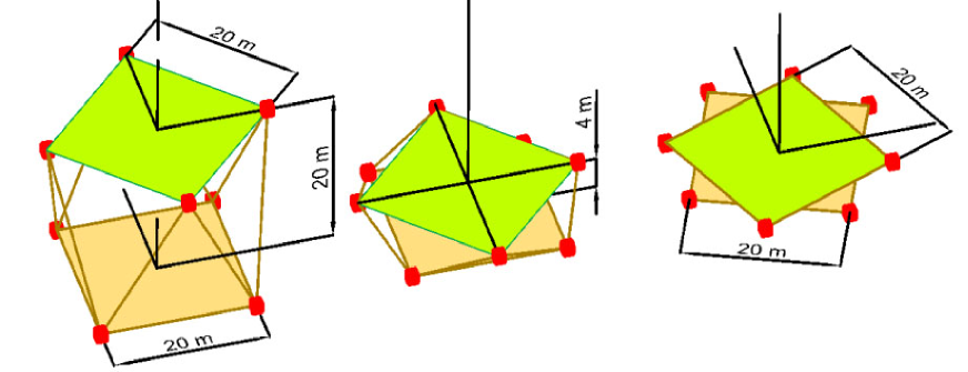
Figure 2:  Three examples of goniometer arranging:
  1) high goniometer – left;  2) low goniometer – center;  3) flat goniometer – right.

Let us consider three simple examples of EAS goniometers for the purpose of illustration. (see Fig.2) The detector number in every example installation is $N_{0}=8$ with the distances between them approximately about $20\>{m}$, as in example in reference [9]. If we locate them in the apexes of squares with edges of $20\>{m}$ length (the radii of both tiers are of $14.1\>{m}$ in size) and estimate the delay periods’ standard error by a rough value of $\sigma=0.5\>m\sim 1.7\>ns$, the aforementioned expression (25) gives us $D_{h}=0.0003125$.

However, let us locate the tiers:

1. with the distance between them equal to $20\>{m}$ (the so-called high goniometer). The dispersion of the “vertical” ort component $D_{z}=D_{h}=0.0003125$;

2. with the distance between the tiers equal to $4\>{m}$ (low goniometer ) and the same configuration of tiers as before. The dispersion of the “vertical” ort component increases: $D_{z}=0.0078125$;

3. with all detectors placed in common horizontal plane (flat goniometer ) at the apexes of a regular octagon with the same circumcircle radius. As before we obtain $D_{h}=0.0003125$. (The “vertical” component is indefinite.)

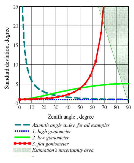
Figure 3: The errors dependencies of spherical angles estimations on the true zenith angle value for all considered cases of the EAS goniometer examples.

The dependencies of angles error estimations on zenith angle value are shown on Fig.3 for all three cases. As one can see, the standard deviation of zenith angle estimation never exceeds the value of $1^{\circ}$ for high goniometer; while for low goniometer it somewhat exceeds $10^{\circ}$ limit only for almost horizontal showers.

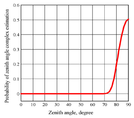
Figure 4: The probability of complex zenith angle estimation.

However, the LAAS group [9] (together with the most part of investigators all over the world) uses the flat goniometer installation. All detectors are placed on the same horizontal plane preventing the possibility of linear estimation of vertical component of EAS direction ort.

On Fig.3 the angle dependencies of error estimations for last flat goniometer example are shown, too. The azimuth angle is measured with the previous accuracy as the detectors’ number and their positions radius have not changed.

The zenith angle estimation error has grown badly. Practically every close-to-horizon angles cannot be measured as there estimations coincide with the horizon within the value of standard deviation. The angles in the shaded area on Fig.3 correspond to this condition. The flat EAS goniometer of the last example is not sensitive for zenith angles larger then $\sim 68^{\circ}$.

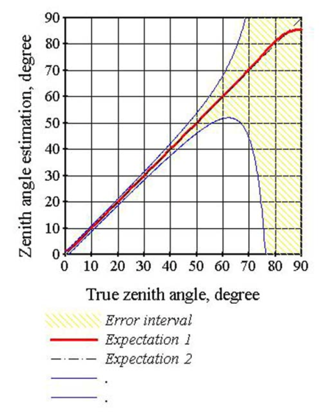
Figure 5: Zenith angle estimation by the flat goniometer:
1) expectation of the flat goniometer estimation through the real part…
2) expectation of the desired consistent and unbiased estimation.

The anticipated probability of dummy complex estimation of zenith angle is shown on Fig.4 for the flat EAS goniometer considered here, as a function of the true zenith angle value. Actually, the estimation can become complex in (nearly) the same shaded area on Fig.3.

The complexity of the zenith angle estimation indicated, caused by the fluctuations of the horizontal components’ estimators, results in the complexity of the expectation value of the vertical component estimator for any value of true zenith angle. The events resulting in complex estimation of the vertical component of the EAS directional ort are plainly rejected in practice. This means the use of the real part of complete estimator (32) for the vertical component estimation. This (real) estimator approaches stochastically the real part of the expectation value of complete estimator $\Re e\textbf{M}(n_{z})$, which does not coincide with the true value of the vertical component. Hence, this estimator on the trimmed sample is biased and inconsistent one. Nevertheless, the use of this value within the interval of angles with negligible probability of complex estimations (Fig.4) is defensible as the angle’s bias value does not exceed the bounds of one standard deviation of the resulting zenith angle (Fig.5).

6 Conclusion.

  The flat kind of goniometer installation has a number of unpleasant properties. When the EAS arrival direction lies far from the zenith, the possibility arises of a complex estimation of the zenith angle with no clear interpretation. The standard error of the last angle grows rapidly to infinity for EAS arrival directions near the horizon. This behavior results in the assertion of an insistent desirability to only use volumetric EAS goniometers, especially for EAS network stations with big angular distances between them. Even a small vertical displacement of part of the detectors in a flat goniometer array (i.e. conversion to low EAS goniometer) fundamentally changes the angles computation conditions: in no case does any complex result arise and the error in zenith angle proves to have a superior limit even for horizontal EAS directions. Finally, the proper detectors arrangement provides the isotropy of errors.

7 Acknowledgments

  The authors are grateful to other current and former members of our group for their technical support. Part of this work was supported by the Georgian National Science Foundation subsidy for a grant of scientific researches #GNSF/ST06/4-075(No 356/07).

References

- [1] Gerasimova N.M. and Zatsepin G.T. 1960 Sov.Phys. — JETP 11 899
- [2] Medina-Tanco G.A. and Watson A.A. 1999 Astropart. Phys. 10 157
- [3] Carrel O. and Martin M. 1994 Phys. Lett. B 325 526
- [4] Fegan D.J et al 1983 Phys. Rev. Lett. 51 2341
- [5] Alexeyev E.N. et al 2002 Astropart. Phys. 17 341
- [6] Florian Goebel for the MAGIC collaboration, arXiv:0709.2605
- [7] J. Holder, the VERITAS collaboration, arXiv:astro-ph/0611598v1
- [8] J. Holder, R.W. Atkins, H.M. Badran at al., arXiv:astro-ph/0604119v1
- [9] N. Ochi et al 2003 J. Phys. G: Nucl. Part. Phys. 29 1169
- [10] G. Korn, T. Korn., Mathematical Handbook …, McGraw Hill Book Company 1968.
- [11] H. Cramèr. Mathematical methods of Statistics. Princeton Univ. Press, N.J. 1958
- [12] W.T.Eadie, D.Dryard, et al. Statistical methods in experimental physics. CERN, 1975
-
[13]
Review of Particle Properties; review: Statistics;
in Physical Review D V50, N3 (Particles and Fields) 1994. -
[14]
A.P. Prudnicov, Yu.A. Brychkov, O.I. Marichev., Integrals and Series,
Moscow, Nauka, 1981 (in russian)