A MULTI-RESOLUTION WEAK LENSING MASS RECONSTRUCTION METHOD

Abstract

Motivated by the limitations encountered with the commonly used direct reconstruction techniques of producing mass maps, we have developed a multi-resolution maximum-likelihood reconstruction method for producing two dimensional mass maps using weak gravitational lensing data. To utilize all the shear information, we employ an iterative inverse method with a properly selected regularization coefficient which fits the deflection potential at the position of each galaxy. By producing mass maps with multiple resolutions in the different parts of the observed field, we can achieve a comparable level of signal to noise by increasing the resolution in regions of higher distortions or regions with an over-density of background galaxies. In addition, we are able to better study the sub-structure of the massive clusters at a resolution which is not attainable in the rest of the observed field. We apply our method to the simulated data and to a four square degree field obtained by the Deep Lens Survey.

1 INTRODUCTION

Recent access to deep, wide field, multi-color optical imaging has established weak gravitational lensing as an effective tool for discovering new clusters of galaxies and measuring the dark matter content of the Universe. Unlike other techniques for selecting clusters, such as observing the X-ray emission by the hot intra-cluster medium, the Sunyaev-Zeldovich effect on the CMB or over-densities of galaxies in coordinate and/or color space, weak gravitational lensing does not rely on the luminous matter and provides a baryon-independent measure of the mass distribution in clusters.

Since the pioneering work of Tyson et al. (1990), significant progress has been made both on the theoretical front (Miralda-Escudé, 1991; Kaiser & Squires, 1993; Squires & Kaiser, 1996; Seitz et al., 1998) and in the quality of the observational data. It is now possible to measure systematic ellipticities as small as 0.005 on scales of many arc-minutes (Parker et al., 2007; Jain et al., 2006; Wittman et al., 2000). However, there are still advances to be made in reconstructing the surface mass distribution in order to create high resolution and accurate mass maps using all of observables such as lens and source redshifts (both spectroscopic and photometric), magnification, and distortion measurements from strong lensing arcs.

In general, there are two classes of reconstruction methods using weak gravitational lensing data: direct and inverse methods. The direct methods, primarily based on the work done by Kaiser & Squires (1993), estimate the surface mass density by approximating a local value for the shear (the tidal gravitational field) from the observed ellipticities of the background galaxies. In these methods, to avoid the divergence of the statistical uncertainty of the surface mass density, the data needs to be smoothed. The smoothing length is a free parameter in the reconstruction and there is no a priori way of determining it.

Furthermore, the transformation of the surface mass density

$$\kappa\rightarrow\kappa^{\prime}=\alpha\kappa+(1-\alpha),$$ (1)

where $\alpha$ is an arbitrary constant does not change the expectation value of the measured ellipticities (Schneider & Seitz, 1995). Due to this degeneracy in the mass sheet, in the absence of redshifts for the sources and lenses, the mass of the clusters cannot be completely determined from the shear information alone. In principle, adding extra information from other observables such as magnification can lift the mass sheet degeneracy (Broadhurst et al., 1995), but this information cannot be simply incorporated in the direct reconstruction methods.

Inverse methods aim to find the best fit to the data (Squires & Kaiser, 1996; Bartelmann et al., 1996) and have previously only been used to study a small number of individual clusters with a low number of background sources. Because of the large number of degrees of freedom, any maximum likelihood analysis of weak lensing data requires some kind of smoothing to reconstruct a mass map. Methods which bin (Bridle et al., 1998) or smooth (Bartelmann et al., 1996) the data to regularize the solution do not use all the information provided by each source galaxy. To utilize all the shear information, one can employ an iterative inverse method which fits for the deflection potential at the position of each galaxy. Applying the smoothing via the a priori expectation of the surface mass density with a properly selected regularization weight is a self-consistent, although computationally expensive way of reconstructing mass maps from the weak lensing data. Furthermore, the magnification information can be simply incorporated in inverse methods by constraining the minimization (Seitz et al., 1998; Bridle et al., 1998). Strong lensing information from observed arcs can be included in the same way (Bradac et al., 2005).

The necessary uniform smoothing of the data in direct methods of reconstruction (and some of the inverse methods) limits the use of the additional information and also produces an inconsistent noise level. The resolution of the mass maps is limited by the strength of the weak lensing signal and the number density of the background sources which varies across the observed field due to Poisson statistics, and also due to background large scale structure. In this paper, we present a regularized maximum likelihood method which can produce a single mass map with multiple resolutions in the different parts of the observed field. Thus, we can achieve a comparable noise level by increasing the resolution at the areas with an over-density of sources. Also, the sub-structure of the massive large clusters which measurably affect the ellipticities of the background galaxies in a vast area can be studied in a map with a resolution which may not be attainable in the rest of the observed field. The lower the shear values, the larger the number of sources that are needed to achieve a consistent signal to noise per pixel across the filed. Therefore, we can create a map with a higher resolution at the areas where the shear values are larger, without reducing the overall spatial signal to noise of the detection.

The only attempt to make a multi-resolution mass map is a multi-scale maximum-entropy method by Marshall et al. (2002) which uses the intrinsic correlation functions with varying width. They report that applying this method to their data did not show a significant difference from the single-scale method they also studied.

The rest of the paper is organized as follows: in § 2, we briefly present the basics of gravitational lensing and in § 3, we describe the details of our technique. In § 4, we test the method with a simulated one square degree field, distorted with five mock clusters and in § 5 we apply it to one of the four square degree fields of the Deep Lens Survey (Wittman et al., 2002). Finally, we summarize our method and describe the future plans in § 6.

2 LENSING RELATIONS

The convergence $\kappa$, the dimensionless surface mass density of a lens, with a projected mass density of $\Sigma(\mbox{\boldmath$x$})$ is defined by $\kappa(\mbox{\boldmath$x$})=\Sigma(\mbox{\boldmath$x$})/\Sigma_{\mathrm{cr}}$, where $\Sigma_{\mathrm{cr}}=({c^{2}}/{4\pi G})\;{D_{\mathrm{s}}}/(D_{\mathrm{d}}D_{\mathrm{ds}})$ is the critical surface mass density, $D_{\mathrm{d}}$ and $D_{\mathrm{s}}$ are the angular diameter distances of the lens and the source from the observer, and $D_{\mathrm{ds}}$ is the angular diameter of the lens from the source. The angular position in the lens plane is denoted by $x$. The convergence is related to the deflection potential $\psi(\mbox{\boldmath$x$})$, by Poisson’s equation $\kappa=\frac{1}{2}\nabla^{2}\psi(\mbox{\boldmath$x$})$. The relation between the deflection potential and the shear is described by two components, $\gamma=\gamma_{1}+\mathrm{i}\gamma_{2}$, where $\gamma_{1}=\frac{1}{2}(\psi_{,11}-\psi_{,22})$ and $\gamma_{2}=\psi_{,12}$, with $\psi_{,ij}=\partial^{2}\psi/\partial x_{i}\partial x_{j}$.

The images are both distorted and magnified. The distortion is due to the tidal gravitational field, described by shear and the magnification is caused by both isotropic and anisotropic focusing, described by both convergence and shear. The ratio of the flux observed from the image and the true flux of the source defines the magnification, given by $\mu=({\det{\mathcal{A}}})^{-1}=({(1-\kappa)^{2}-|\gamma|^{2}})^{-1}$.

To study the effects of gravitational lensing on background sources, an ellipse is fitted to the shape of each galaxy. The complex ellipticity of a source is defined by the brightness quadrupole moments $Q_{ij}$ as $\epsilon=(Q_{11}-Q_{22}+2\mathrm{i}Q_{12})/(Q_{11}+Q_{22})$. The transformation between the image’s quadrupole moments $Q^{(i)}$ and the source’s moments $Q^{(s)}$ due to gravitational lensing is given by $Q^{(i)}=\mathcal{A}\;Q^{(s)}\;\mathcal{A}$ (Kaiser & Squires, 1993), where $\mathcal{A}$ is the Jacobi matrix

$$\mathcal{A}=(1-\kappa)\;\left(\begin{array}[]{cc}1-g_{1}&-g_{2}\\ -g_{2}&1+g_{1}\\ \end{array}\right).$$ (2)

The parameter $g=\gamma/(1-\kappa)$ is the reduced shear. The transformed shapes of objects does not depend on the convergence and shear separately, but on the reduced shear. This means $\kappa$ and $\gamma$ are not direct observables and only their combination in $g$ (or a function of $g$) can be measured from image ellipticities. The shapes are also invariant under the transformation $g\rightarrow 1/g^{*}$, so one can define the complex distortion as

$$\delta=\frac{2g}{1+|g|^{2}}\;,$$ (3)

which is invariant under a such transformation (Schneider & Seitz, 1995).

3 THE METHOD

In this regularized maximum-likelihood method, our goal is to describe the surface mass density distribution over the observed field by fitting for the deflection potential on a multi-resolution grid. We have adapted the prescription of Seitz et al. (1998) in constructing the grid of the deflection potential in order to accommodate for the multi-resolution fitting. In a regular maximum-likelihood method, a $\chi^{2}$ term of the form

$$\chi^{2}=\frac{1}{N_{g}}\;\sum_{k=1}^{N_{g}}\frac{\left(\epsilon_{k}-\langle\epsilon\rangle(\mbox{\boldmath$x$}_{k})\right)^{2}}{\sigma_{\epsilon}}$$ (4)

is minimized, where $N_{g}$ is the number of galaxies, $\epsilon_{k}$ is the measured complex ellipticity of galaxy $k$ located at $\mbox{\boldmath$x$}_{k}$ ($1\leq k\leq N_{g}$), and $\langle\epsilon\rangle(\mbox{\boldmath$x$}_{k})$ is the expectation value of the average ellipticity at $\mbox{\boldmath$x$}_{k}$ which depends on the deflection potential and its derivatives at that point. Should the source redshift information be provided, the expectation value of the ellipticity could be modified with a cosmological weight function (Lombard & Bertin, 1999).

Due to the unmeasurable intrinsic elliptical shape of the weakly distorted galaxies, each single object does not provide enough information for lensing reconstruction. Despite this, the number of degrees of freedom in minimizing $\chi^{2}$ is nominally the number of data points (i.e. galaxies) subtracted by the number of fitting points. Therefore, the degrees of freedom in a wide field reconstruction is quite large and minimizing $\chi^{2}$ by itself, gives $\psi$ enough freedom to be able to make it unrealistically small which yields to a potential that reconstructs the noise in the data and results in a wrong solution. Adding a regularization term with a proper weight helps to constrain $\chi^{2}$ and avoid over-fitting it. In our method, we minimize a function of $\psi$ defined as

$$\mathcal{F}=\frac{1}{2}\chi^{2}+\lambda\;\mathcal{R}\;,$$ (5)

where $\lambda$ is the regularization coefficient. The $\chi^{2}$ is regularized with a modified zeroth-order regularization function

$$\mathcal{R}=\sum_{m=1}^{N_{x}}\;\sum_{n=1}^{N_{y}}({\kappa}_{mn}-{p}_{mn})^{2}\;,$$ (6)

where $\kappa_{mn}$ is the surface mass density at the grid points of the reconstruction grid and ${p}_{mn}$ is the prior. The main advantage of using this function compared to the entropy inspired regularization functions is its simplicity. In principle, the entropy inspired functions guarantee $\kappa$ to be a positive number. But in real numerical analysis when $\kappa$ becomes very small, these functions and their derivatives do not behave smoothly. Furthermore, in the presence of a mass-sheet degeneracy, it is not clear that enforcing the positivity of kappa is useful in deriving a solution. Choosing a function as simple as $\mathcal{R}$ which is zero when $\kappa$ is equal to the prior is sufficient and ensures the smoothness of the reconstruction.

The magnification information can be included by adding to $\mathcal{F}$, a $\chi^{2}_{\mu}$ term of the form

$$\chi^{2}_{\mu}=\frac{1}{N_{\mu}}\;\sum_{l=1}^{N_{\mu}}\frac{\left(\mathcal{M}_{l}-\mu(\mbox{\boldmath$x$}_{l})\right)^{2}}{\sigma_{\mu}},$$ (7)

with $N_{\mu}$ number of magnification data points $\mathcal{M}_{l}$ located at $\mbox{\boldmath$x$}_{l}$ where the predicted value of magnification is given by $\mu(\mbox{\boldmath$x$}_{l})$.

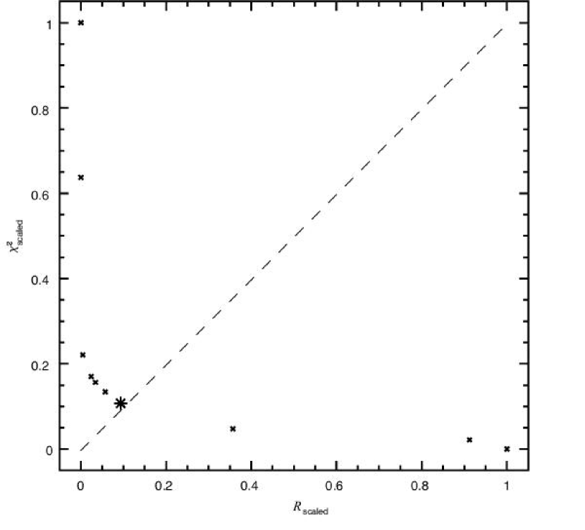
Figure 1: The resulting $\chi^{2}_{\mathrm{scaled}}$ vs. $\mathcal{R}_{\mathrm{scaled}}$ from 9 minimizations with coefficients between $\lambda=0$ and $\lambda=10$ in addition to the result from minimizing only $\mathcal{R}$. The intersection between the $\chi^{2}_{\mathrm{scaled}}$-$\mathcal{R}_{\mathrm{scaled}}$ curve and the line $\chi^{2}_{\mathrm{scaled}}=\mathcal{R}_{\mathrm{scaled}}$ indicates $\lambda=0.001$ to be the proper coefficient for the $1^{\prime}.5$ per pixel reconstruction of the simulated field.

The parameter $\lambda$ in equation (5), known as the regularization coefficient, represents the compromise between the best fit (i.e the answer that minimizes $\chi^{2}$) and the closest match to the prior knowledge (i.e. the answer that minimizes $\mathcal{R}$). A proper way of finding the best value for the regularization coefficient has been the subject of much debate. For instance, Seitz et al. (1998) constrain $\chi^{2}$ to be equal to the degrees of freedom in order to find a good guess for $\lambda$. It is however not clear what a “degree of freedom” is. Because each galaxy shape is mostly due to the intrinsic galaxy ellipticity, the effective number of degrees of freedom per galaxy is much less than 1. Bridle et al. (1998) derive a value for $\lambda$ in a Bayesian manner, which also has the disadvantage of not easily adapting to the data in a realistic numerical analysis. Whatever method employed, the value of the regularization coefficient must be low enough so that the solution follows the data and high enough so that it avoids the numerical artifacts caused by over-fitting. To determine this value, we minimize $\mathcal{F}$ as a function of $\lambda$ and compare the resulting $\chi^{2}$ versus $\mathcal{R}$ by scaling them to values between 0 and 1. The minimum value of $\chi^{2}$ is obtained when $\lambda=0$ (the best fit solution, corresponding to $\chi^{2}_{\mathrm{scaled}}$ of 0 and $\mathcal{R}_{\mathrm{scaled}}$ of 1), and its maximum value is obtained when only $\mathcal{R}$ is minimized (the smoothest solution, corresponding to $\chi^{2}_{\mathrm{scaled}}$ of 1 and $\mathcal{R}_{\mathrm{scaled}}$ of 0.) The intersection between $\chi^{2}_{\mathrm{scaled}}$ vs. $\mathcal{R}_{\mathrm{scaled}}$ curve and the line $\chi^{2}_{\mathrm{scaled}}=\mathcal{R}_{\mathrm{scaled}}$ determines the proper value of the regularizaion coefficient as shown in Figure 1. It should be noted that this method dictates approximately equal weights to the $\chi^{2}$ term and the regularization term. However, a different level of agreement with the prior knowledge (in our case, smoothing) is achieved by selecting an intersecting line that has a different slope. Despite the fact that this method requires a fair amount of computation time, it ensures the agreement between the data and the a priori expectation.

Our goal is to apply this method to the wide field optical data obtained by the Deep Lens Survey. Because the analytical expectations for the average ellipticities of galaxies do not take the noise in the data and the shape measurements into account, we estimate the expectation value of the average ellipticities as a function of shear based on the simulated data.

In our first suite of simulations, we produce a series of 17.36 square arc-minute simulated fields in which the simulated galaxies are distributed between magnitudes of 22 and 25.5 in the $R$ band. This is approximately the magnitude range of the objects used from the DLS data for the mass reconstruction analysis. The ellipticity distribution of the simulated galaxies is assumed to be the ellipticity distribution of the galaxies in the UDF (Beckwith, 2005). Because of the small PSF and high signal to noise detection in the UDF data, the measured shapes are nearly accurate estimates of the real shapes of the galaxies. Therefore, despite the uncertainties due to the finite number of galaxies, the derived ellipticity distribution is a fair approximation. To include as many galaxies as possible, we assume that their average shape does not depend on redshift. We choose the $V$ band data of the UDF to determine the ellipticity distribution, because it has the highest signal to noise and is close in wavelength to the $R$ band of the Deep Lens Survey, where the shapes of our sources are measured. In total, we generate $\sim$ 120,000 simulated galaxies to estimate the expectation value of the ellipticity as a function of distortion.

We distort the simulated fields according to equation (2), varying $0\leq g_{1}\leq 0.6$, while $g_{2}$ is fixed at zero. This distortion step is performed at the pixel-scale of the UDF (0.03 arc-seconds). The DLS’ PSF is almost always well-sampled, therefore, the simulated images are first linearly transformed onto the DLS pixel-scale (0.25 arc-seconds) and then smoothed with a Gaussian to simulate the 0.9 arc-second seeing of the data. An appropriate background noise is also added to match the simulations to the properties of the actual deep field images.

Encouragingly, $\langle\epsilon_{2}\rangle$ averages to zero and only $\langle\epsilon_{1}\rangle$ increases with shear in our simulations. This demonstrates that it is correct to assume that $\epsilon_{1}$ and $\epsilon_{2}$ have the same orientation as $g_{1}$ and $g_{2}$. To avoid the degeneracy between $g$ and $1/g^{*}$, we use the distortion parameter introduced in equation (3) and define $\langle\epsilon\rangle(\mbox{\boldmath$x$}_{k})=f(|\delta|^{2})\delta$. The function $f(|\delta|^{2})$ is found from the simulations (where $g_{2}=0,\delta_{2}=0$) by

$$f(|\delta|^{2})=\langle\epsilon_{1}\rangle/\delta_{1}\;.$$ (8)

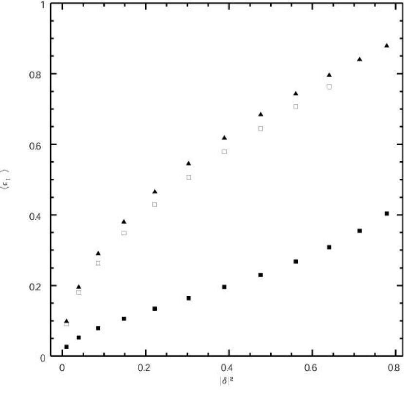
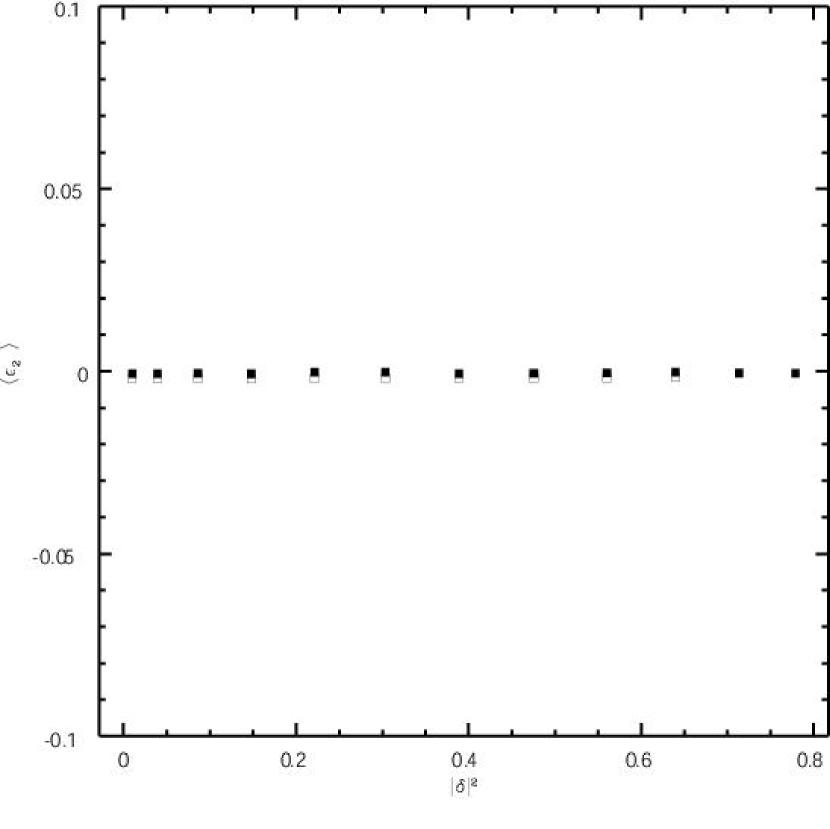
Figure 2: The expectation value of $\epsilon_{1}$ and $\epsilon_{2}$ versus $|\delta|^{2}$. Solid squares represent the simulations at the DLS pixel-scale with simulated PSF and matched signal to noise, open squares represent the simulations of a UDF like field and solid triangles represent the analytically approximated expectations (Schneider & Seitz, 1995).

The derived expectation values from our simulations along with the analytical approximations (Schneider & Seitz, 1995) are shown in Figure 2. Using the same set of simulations, we also determine the dispersion in the ellipticity of galaxies $\sigma_{\epsilon}$ as a function of distortion.

Once one exceeds a shear value of 0.6, the shapes of more than 50 per cent of the objects in the simulations are not well measured due to splitting by the detection software. This causes a bias in the expected ellipticity estimates. Therefore, we extrapolate and use $f(|\delta|^{2})$ and $\sigma_{\epsilon}$ derived from $|\delta|\leq 0.88$ distortions for the higher values as well. This extrapolation is acceptable, because real highly elliptical galaxies are very rare (while high measured ellipticities are most often caused by unresolved blends of multiple galaxies). Therefore, we can and do filter them out of the data without losing any significant weak lensing information.

4 IMPLEMENTATION OF THE METHOD

To create a $N_{x}\times N_{y}$ map of the surface mass density distribution, the observed field is covered with a $(2N_{x}+4)\times(2N_{y}+4)$ grid of the deflection potential $\psi_{ij}$. Because the convergence and shear are second order derivatives of the deflection potential, adding a constant or a linear term in $x$ to $\psi$ leaves them unchanged and $\psi$ needs to be constrained to be constant at four of the grid points. For computational simplicity, we have decided to keep the four corners of the grid fixed.

The values of the shear $\gamma_{ij}$ and convergence $\kappa_{ij}$ at the grid points are obtained by second order finite-differencing, hence, the extra rows and columns at each side of the grid. The values of shear and convergence at the position of each galaxy in the data are calculated via bilinear interpolation. The shear and convergence are computed locally and the coefficients relating the deflection potential to $\kappa(\mbox{\boldmath$x$}_{k})$ and $\gamma(\mbox{\boldmath$x$}_{k})$ depend only on the geometry of the grid and the location of the galaxy at $\mbox{\boldmath$x$}_{k}$, therefore, the coefficients can be calculated once and stored to speed up the computations.

To compute the regularization function $\mathcal{R}$, we need to know the values of $\kappa_{mn}$. To fix the ringing effects in the projected mass maps caused by second order numerical differentiation of $\psi$, we block average $\psi_{ij}$ at four neighboring grid points and then take the derivatives of the deflection potential on this new grid. Hence, the size of the final mass map is $N_{x}\times N_{y}$.

The components of the shear are also computed on the block averaged deflection potential grid. Because $\mathcal{M}_{l}$ are scattered on the field and are not necessarily located on the grid points, the matrix $\mathcal{H}_{l}^{mn}$ is defined to determine the amount by which each grid point is weighted to compute the expected magnification at $\mbox{\boldmath$x$}_{l}$, changing equation (7) to

$$\chi^{2}_{\mu}=\frac{1}{N_{\mu}}\;\sum_{l=1}^{N_{\mu}}\frac{1}{{\sigma_{\mu}}}\;\left(\mathcal{M}_{l}-\sum_{m,n=1}^{N_{x},N_{y}}\mathcal{H}_{l}^{mn}\mu_{mn}\right)^{2}.$$ (9)

The elements of $\mathcal{H}$ only depend on the positions of the magnification data and the structure of the grid. Therefore, they too can be calculated once and stored, speeding up the analysis. In the presence of magnification data, $\psi$ needs to be constrained to be constant only at three grid points.

To minimize $\mathcal{F}$, we use a conjugate-gradient method as encoded in the frprmn routine by Press et al. (1992). We need to provide this algorithm the first derivatives of $\mathcal{F}$ with respect to $\psi_{ij}$ which can be derived with a combination of analytical and numerical methods. In general,

$$\frac{\partial\mathcal{F}}{\partial\psi_{ij}}=\frac{\partial\mathcal{F}}{\partial\gamma_{1}(\mbox{\boldmath$x$}_{k})}\times\frac{\partial\gamma_{1}(\mbox{\boldmath$x$}_{k})}{\partial\psi_{ij}}+\frac{\partial\mathcal{F}}{\partial\gamma_{2}(\mbox{\boldmath$x$}_{k})}\times\frac{\partial\gamma_{2}(\mbox{\boldmath$x$}_{k})}{\partial\psi_{ij}}+\frac{\partial\mathcal{F}}{\partial\kappa(\mbox{\boldmath$x$}_{k})}\times\frac{\partial\kappa(\mbox{\boldmath$x$}_{k})}{\partial\psi_{ij}}\;.$$ (10)

The derivatives of $\kappa$, $\gamma_{1}$ and $\gamma_{2}$ with respect to $\psi_{ij}$ only depend on the geometry of the grid and the position of the galaxies. They can be derived from the stored coefficients which relate the convergence and two components of shear to the deflection potential at the grid points.

The reconstruction procedure starts at a low resolution which depends on the area and the number of galaxies of the data. At this level the mass maps are smooth enough and the regularization is not required ($\lambda=0$). At the end of this step, two very coarse maps of the surface mass density and the deflection potential are produced. To increase the resolution, we linearly expand and smooth the maps with a Gaussian function ($\sigma=1$ pixel, equal to the inherent correlation length of the maps) and use the map of $\psi$ as the initial potential and the map of $\kappa$ as the prior map of the second minimization.

By finding the proper value of $\lambda$, we are able to increase the resolution to the limit that the data allows us. The resolution of a mass map is limited by the strength of the weak lensing signal and the number density of the background sources which varies across the observed field due to a variation in source counts and possible background large scale structure. To obtain the highest possible resolution, the second step can be repeated: expanding and smoothing the $\psi$ and $\kappa$ maps of the previous reconstruction and using them as the initial potential and prior, respectively.

In principle, in a maximum likelihood method, the number of unknowns (values of the deflection potential on the grid points) must be at least the number of equations (the measured ellipticities of the galaxies). However, one single galaxy in the weak lensing limit does not provide enough shear information for one grid point because its ellipticity tensor is dominated by the random component. Additionally, the Poisson variation in source counts and the noise in the shape measurements have undetermined effects on the signal to noise across the field. Furthermore, the numerical artifacts in minimizing $\mathcal{F}$, which also limit the resolution are not well predicted. A maximum resolution for a given data set can be approximated based on its number of source galaxies, but an exact final resolution of the mass maps can not be predetermined. If the signal to noise in a map is not sufficient, we are bound to decrease its overall resolution, though we may be able to maintain a high resolution at some parts of the field with our multi-resolution reconstruction technique.

The multi-resolution grid is essentially the same as the single-resolution grid described earlier. It only requires an extensive amount of bookkeeping at the edges of the sub-grid regions. The shear and convergence computations for the galaxies in the middle regions of the sub-grids are performed similarly to the single-resolution computations. For the galaxies which lie on the edge or corner cells, the values of the deflection potential at the required positions in the field with no real grid points allocated for them are interpolated. As in the single-resolution construction, the coefficients relating the convergence and shear to the deflection potential depend only on the position of the galaxies and the geometry of the main grid and the sub-grids, thus this step is required to be performed only once.

In order to simplify the calculations, the resolutions of the rectangular sub-grids, which may be different from one to another, are required to be 2$n$ times higher than the original resolution. The maps of $\psi$ and $\kappa$ produced in the final single-resolution reconstruction are used as the initial potential and the prior, respectively. The proper regularization coefficient is derived similarly to the single-resolution reconstruction. The minimization of the function $\mathcal{F}$ is performed over all grid points in the main grid and sub-grids, except for the four corners that are held constant.

5 SIMULATED DATA

We simulate a one square degree field distorted by 5 clusters with the NFW profile (Navarro, Frenk & White, 1997) at a redshift of 0.4 with masses ranging between $10^{13}$ to $10^{15}$ Solar masses. The mass and position of each cluster is detailed in Table 1 and the analytical expectations of the surface mass density map due to these clusters is shown in Figure 3 (top left). Clusters number 1 and 2 are chosen to be close to each other to test our ability to separate bright adjacent peaks using the multi-resolution method. Cluster number 3 is a typical isolated cluster and clusters 4 and 5 are are intentionally chosen to be low-mass clusters to study the lower signal to noise limits of the reconstruction by our technique.

The angular diameter distances are evaluated assuming a $\Lambda$CDM cosmology with $\Omega_{m}=0.3$, $\Omega_{\Lambda}=0.7$, and the Hubble constant $H_{0}=70\;\mathrm{km}\;\mathrm{s}^{-1}\;\mathrm{Mpc}^{-1}$. The objects are randomly oriented galaxies. The ellipticity distribution is assumed to be the ellipticity distribution of the galaxies in the UDF and their number density follows a power law distribution (Tyson, 1988). The galaxies are divided between seven redshift layers based on their magnitudes, which range between 23 and 27 in the $R$ band: $z_{1}=0.27$, $z_{2}=0.45$, $z_{3}=0.68$, $z_{4}=0.90$, $z_{5}=1.20$, $z_{6}=1.95$ and $z_{7}=3.00$. These logarithmically determined layers fairly simulate the redshift distribution of the galaxies in the Deep Lens Survey and varying these values, especially the furthest redshift, does not change the total distortion by a measurable amount. After distorting, we convolve the image to a seeing of 0.9 arc-seconds.

To measure the shape of the galaxies, we employ the same procedure used in the Deep Lens Survey’s pipeline (Wittman et al., 2006). Briefly, we use SExtractor (Bertin & Arnouts, 1996) to detect the objects. The improve upon the shape measurements which are not optimal for weak lensing studies, we employ the ellipto program, which can produce more accurate shape measurements via an iterative weighting algorithm, where the weight function is an elliptical Gaussian (Bernstein & Jarvis, 2002). We apply the same selection criteria in magnitude and size applied to the DLS data to select objects to be used in making the mass maps (Wittman et al., 2006). We require that the moments be successfully measured by ellipto and employ the size measure defined by Bernstein & Jarvis (2002) to filter out the objects smaller than the PSF (ellipto-size of $5\;\mathrm{pixel}^{2}$). We only keep the objects brighter than the magnitude 25.5. After filtering out the unwanted objects, we have a catalog of $\sim$ 109,000 galaxies.

We start off the reconstruction at a resolution of 3 arc-minutes per pixel on the grid of the deflection potential with a constant initial value over the field which yields a mass map with a 6 arc-minute per pixel resolution. At this level, the maps are coarse enough that there is no need for any regularization, hence $\lambda=0$. To find the proper regularization coefficient for the higher resolution reconstructions we follow our recipe and run minimizations with coefficients between $\lambda=0$ and $\lambda=10$ in addition to minimizing only $\mathcal{R}$ at each step to finally produce a $1^{\prime}.5$ per pixel mass map. Figures 1 and 3 (top right) show $\chi^{2}_{\mathrm{scaled}}$ vs. $\mathcal{R}_{\mathrm{scaled}}$ for the last step of this reconstruction process and the final mass map, respectively. Although we do not probe the entire parameter space directly at the highest resolution, we vary the values of the deflection potential evenly over the lowest resolution grid with small and large increments which does not produce a lower $\chi^{2}$, assuring that the conjugate-gradient method reaches the minimum and does not stop at a possible local minima.

Due to the low signal to noise detection of the lowest mass clusters, it is not possible to increase the resolution of the overall map. However, it is still possible to increase the resolution at the vicinity of the first and second clusters, where we increase the resolution of the mass map in a square region by a factor of two to $0^{\prime}.75$ per pixel. In the single-resolution map, these clusters are reconstructed without any separation (i.e. as a single object). The resulting multi-resolution convergence map (Fig. 3, bottom right) shows the cluster not only with the expected symmetric profile, but also very well separated (with the peaks detected at $2^{\prime}.65$ of each other, in very good agreement with the $2^{\prime}.9$ separation of the input profile).

Because of the differential nature of our fitting function, the pixels of the mass maps created by our method are not strongly correlated with each other. Therefore, the total surface mass density of each deflector can be measured by summing over the values of the pixels which are above a predetermined threshold. We measure $\kappa_{\mathrm{total}}$ within the $r_{200}$ radius of each deflector, setting the detection threshold at 2 times the background rms. At this threshold level, all five deflectors along with three spurious objects are detected. Obviously, increasing the detection threshold will remove the spurious objects, however, the weakest deflector would not be detected either (for instance at 3 times the background rms). In the absence of other observational data such as redshift or magnification information, the mass sheet degeneracy cannot be broken. Nonetheless, our measurements (Table 2) are in close agreement in positions and total surface mass densities with the measurements from an analytically calculated map of convergence (Fig. 3, top left) (Wright & Brainerd, 2000). A mass sheet corresponding to the degeneracy coefficient of $\alpha\sim 0.88$ (Eqn. 1) transforms the measured surface mass density to the expected surface mass within the estimated errors. The effects of this degeneracy in our inverse method are most probably suppressed, because the reconstruction process is started with the assumption that the field is empty of any structure. This is an initial condition that cannot be incorporated in a direct method reconstruction.

We also reconstruct the convergence map of a catalog made by distorting the same simulated source galaxies with five deflectors located at the same position but with half the strength (i.e. the $M_{200}$ mass of each cluster is reduced by half.) As expected (Bridle et al., 1998), the noise level and the regularization coefficient at each step of the reconstruction remain the same as the original reconstruction process. However, the two weakest deflectors are not detected at all when the detection threshold is set at 3 times the background rms. We similarly reconstruct the convergence map of a catalog distorted by the original deflectors but with only half the background galaxies. The change in the number of sources also changes the regularization coefficient. After determining the proper value of $\lambda$ and making the final mass map, the measured signal of the three more massive clusters is very close to the signal measured from the original mass map while the two least massive ones are not detected.

In addition, we reconstruct the surface mass density employing a direct method (Kaiser & Squires, 1993; Wittman et al., 2006), using the weight function introduced by Fischer & Tyson (1997)

$$W(r)=(1-e^{-\frac{1}{2}({r^{2}}/{r^{2}_{\mathrm{in}}})})\;e^{-\frac{1}{2}({r^{2}}/{r^{2}_{\mathrm{out}}})},$$ (11)

with $r_{\mathrm{in}}=1^{\prime}.1$ and $r_{\mathrm{out}}=12^{\prime}.5$. The atmospheric and optical distortions of the shapes of the background sources result in suppressed signals. We correct for these effects by employing the method introduced by Bernstein & Jarvis (2002) and approximate the amount of required adjustments to the ellipticities of each source galaxy. In the resulting mass map (Fig. 3, bottom left), when the detection threshold is set at 2 times the background rms, we are able to detect all five deflectors along with nine spurious objects.

The pixels in the direct method map are highly correlated. Moreover, because of the weight function (Eqn. 11), it is the convolved surface mass density that is measured from this map. Therefore, it is not proper to compare the $\kappa_{\mathrm{total}}$ measurements with the previous measurements, and thus the direct reconstruction map is only suitable to study the number count of clusters and possibly the relative strength of their signal.

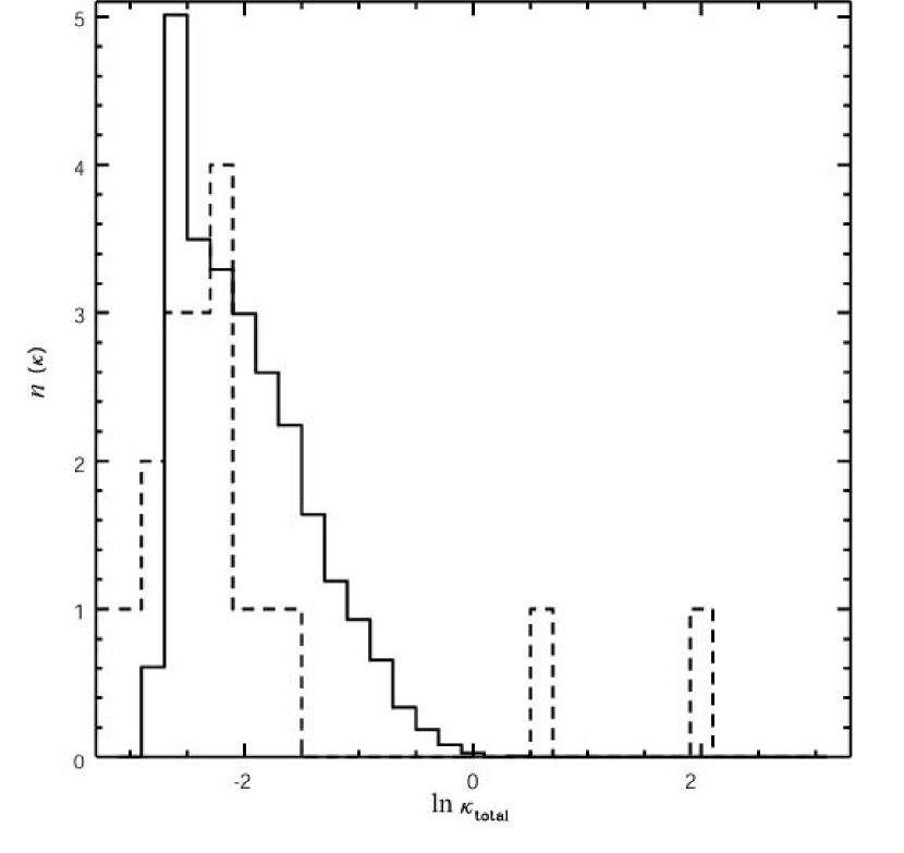
Figure 4: The histogram of the number of detected objects $n(\kappa)$ per catalog for a given total surface mass density $\kappa_{\mathrm{total}}$. The solid histogram shows $n(\kappa)$ for the Monte Carlo catalogs base on the simulated field catalog (made by shuffling the ellipticities of the source galaxies in the simulated field) and the dashed histogram shows $n(\kappa)$ for the original simulated catalog.

To estimate the statistical significance of detecting clusters at different resolutions given our data, we perform a set of Monte Carlo simulations and create a number of source catalogs in which the ellipticity components of one galaxy is given to another, though their positions are not changed. The mass map for each catalog is created by starting at the initial resolution of the original mass map and the same procedure is followed to achieve the final resolution using the same regularization coefficients of the original reconstruction process at each step. Figure 4 shows that there are not any objects in the Monte Carlo catalogs with signals larger than or equal to the combined signal of the first and second clusters, where the detection threshold is set at 1.5 times the background. This is also true for the third cluster. The histogram in Figure 4 can also be interpreted as the probability distribution that the peaks are real detections. We calculate the probability of measuring a signal within the $r_{200}$ radius of each deflector that is equal to its $\kappa_{\mathrm{total}}$ by measuring the probability of finding the same signal in randomly selected regions of the Monte Carlo mass maps (Table 2). When there are no detected objects with a given signal, a rough lower limit for the probability of detection being real can be estimated by the inverse of the number of the Monte Carlo simulations per detected objects in the original catalog with that signal (Wall & Jenkins, 2003, and references within). In addition, because the $r_{200}$ of each cluster is a known priori, we can estimate the 1-$\sigma$ error for the measured total surface mass density of the clusters, using the same set of Monte Carlo simulations. This Monte Carlo analysis shows that we have been able to detect the more massive clusters with a high probability of being real detections and also measure their total surface mass density in good agreement with the analytical input. The total surface mass density measurements for the lower mass clusters are also in good agreement with the analytical input. However, the high number of detected objects in the Monte Carlo simulation with similar signals to those of the less massive clusters, suggests a lower probability that any detection peak is a real object.

6 WIDE FIELD OPTICAL DATA

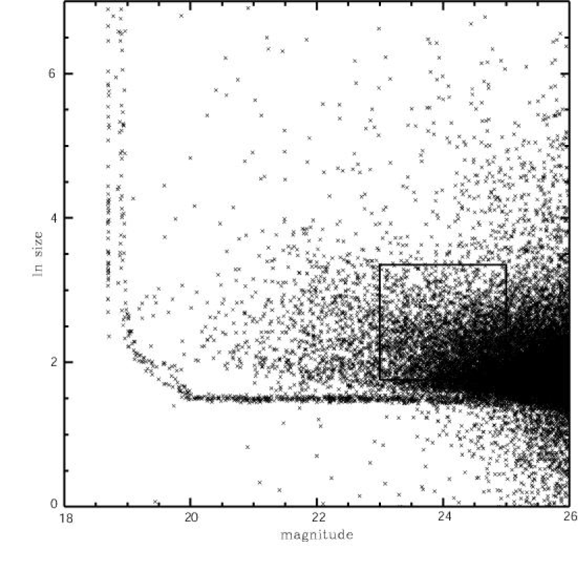
Figure 5: The ellipto-size vs. magnitude diagram of the objects in a random $0.1\deg^{2}$ region of the DLS F2. To clean the data of unsuitable objects for the weak lensing analysis, stars and any object smaller than the PSF size, along with the bright end of the locus which contains saturated objects and bright galaxies are filtered out. We also only keep the galaxies with successfully measured intensity moments (by ellipto) that are brighter than $R=25$, selecting only the objects inside the box to be consistent with the selection method of Wittman et al. (2006).

We also apply our method to reconstruct the mass distribution over a $4\deg^{2}$ field with deep optical imaging ($R\leq 26$), obtained by the Deep Lens Survey. The DLS is a multi-color survey of five separate patches of sky with a consistently good image quality ($\leq 0.9^{\prime\prime}$) in the $R$ band (where the shapes of the source galaxies are measured). We do not intend to break the mass sheet degeneracy in this paper and only use the shear information in the data. We run our method on the DLS field 2 (F2) centered at RA = $09^{h}19^{m}32^{s}.4$, DEC = $+30^{\circ}00^{\prime}00^{\prime\prime}$. For the weak lensing analysis, the data is cleaned of unsuitable objects (Wittman et al., 2006). Stars and any object smaller than the PSF size are removed, using the ellipto-size vs. magnitude diagram. The bright end of the locus which contains saturated objects and bright galaxies is also filtered out. We also only keep the galaxies with successfully measured intensity moments (by ellipto) which are brighter than $R=25$ to reduce the noise due to the faintest and noisiest galaxies. After filtering the unwanted objects out, there are $\sim$ 140,000 galaxies left in the data set (Fig. 5).

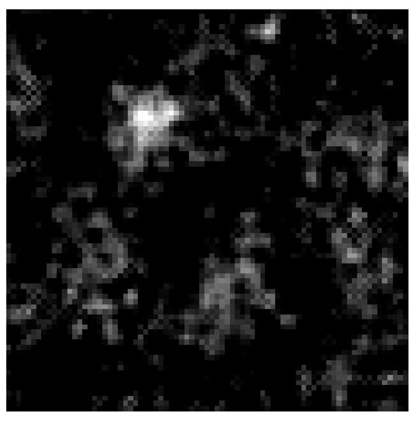
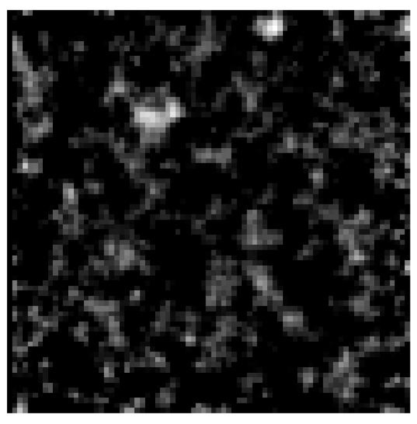
Figure 6: The final single-resolution convergence maps of the $4\deg^{2}$ DLS F2, from the inverse (left) and the direct (right) reconstructions, with a resolution of $1^{\prime}.5$ per pixel.

In the same way as described in the previous section, we start the reconstruction process at a very low resolution of 6 arc-minutes per pixel without regularizing the $\chi^{2}$, that produces a 12 arc-minute per pixel mass map. The process is continued and the higher resolution mass maps with the appropriate regularization coefficients are created. After four steps, the final mass map with a resolution of $1^{\prime}.5$ per pixel is created (Fig. 6, left). This figure (right) also shows the direct mass reconstruction of this field with $r_{\mathrm{in}}=2^{\prime}.9$ and $r_{\mathrm{out}}=24^{\prime}.4$ (Eqn. 11).

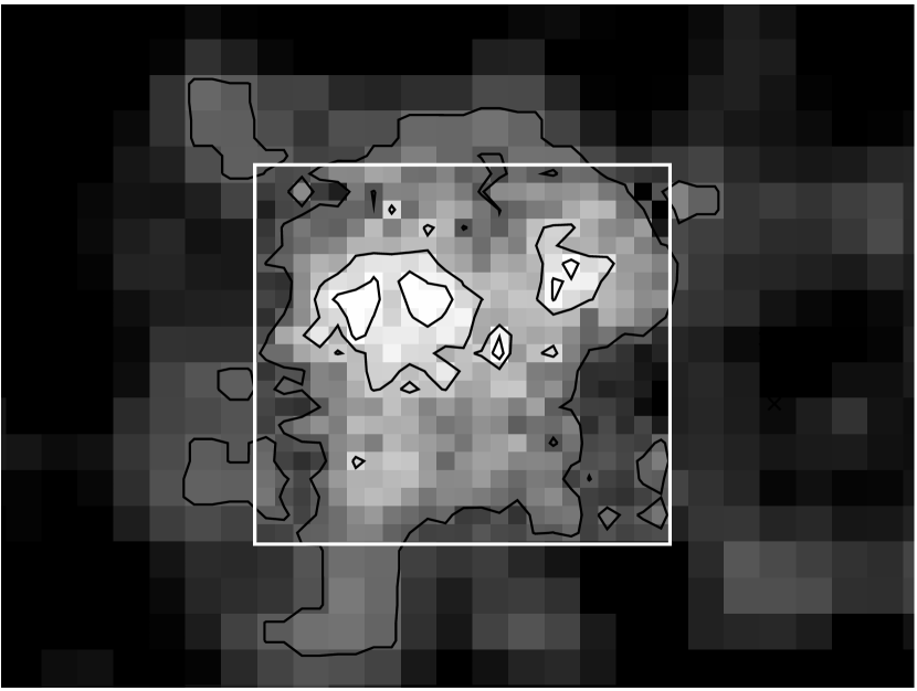
Figure 8: The section of the final multi-resolution convergence map of the DLS F2 (Fig. 7) in the vicinity of the the A781 complex with overlayed intensity contours. The resolution in the box around the A781 complex is $0^{\prime}.75$ per pixel whereas the resolution in the rest of the field is $1^{\prime}.5$ per pixel.

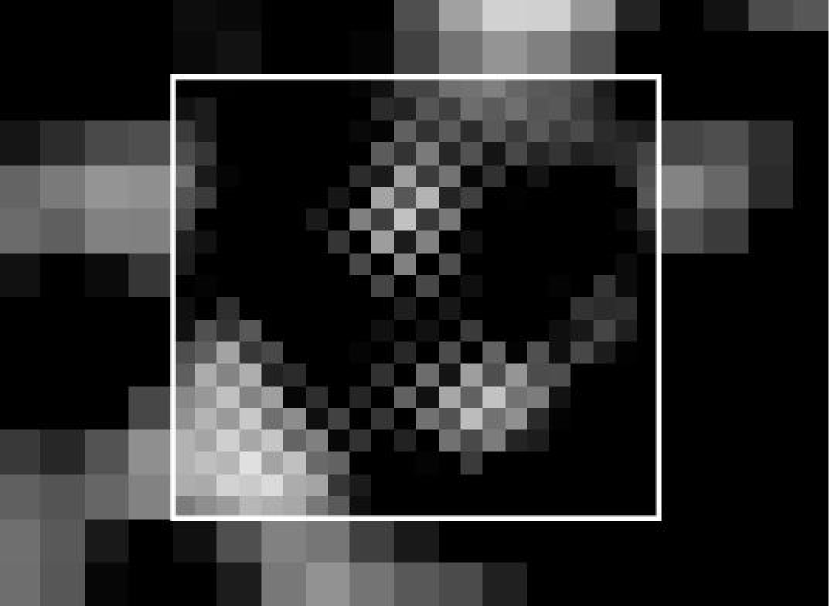
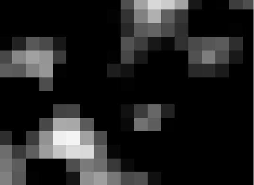
Figure 9: The sections of the multi-resolution reconstruction of a random region (left) and the original single-resolution reconstruction of the same region (right) of the DLS F2. This region is void of areas with large signal. The resolution in the box is $0^{\prime}.75$ per pixel whereas the resolution in the rest of the field is $1^{\prime}.5$ per pixel. It is clear that in the multi-resolution region, it is the noise that has been fitted for rather than the signal, indicating that a higher global resolution is not attainable with this source catalog.

The largest signal in this field is due to a set of known clusters (the Abell 781 complex) which consists of several independent components at redshifts of 0.29-0.43 (Geller et al., 2005). In the final single-resolution mass map, the sub-structure of this system is not very well resolved. However, the signal due to this complex is high enough to allow a higher resolution reconstruction which the rest of the field does not permit. Therefore, an area ($0.09\deg^{2}$) around this region for the multi-resolution reconstruction is chosen. The resulting mass map is shown in Figures 7 and 8, in which three out of the four spectroscopically confirmed components of this system are very well resolved. Two other bright peaks also appear in the vicinity of this system, which will require more investigation to be confirmed. We also perform the multi-resolution reconstruction on two random regions of this field void of areas with large signal. The result is mass maps in which the noise has been fitted for rather than the signal, showing that a higher global resolution is not attainable with this source catalog (Fig. 9).

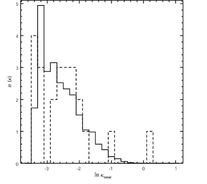
Figure 10: The histogram of the number of detected objects $n(\kappa)$ per catalog for a given total surface mass density $\kappa_{\mathrm{total}}$. The solid histogram shows $n(\kappa)$ for the Monte Carlo catalogs base on the DLS field catalog (made by shuffling the ellipticities of the source galaxies in the simulated field) and the dashed histogram shows $n(\kappa)$ for the original DLS F2 catalog.

The same Monte Carlo method described earlier is employed to estimate the statistical significance of detecting clusters in this field. Neither the $r_{200}$ radii nor the redshifts of the cluster candidates in this field are a priori known. Therefore, we measure the total isophotal signal, setting the detection threshold is set at 1.5 times the background rms. Figure 10 shows the number of the detected objects with a given total signal per catalog. This graph indicates that the number of detected objects per catalog with signals larger than or equal to those of the top two cluster candidates is insignificant, thus they are detected with very high signal to noise and their realness is highly probable. However, the high number of objects per one Monte Carlo catalog with signals equal to the lower ranking objects in the DLS field suggests that these objects have a much lower probability of being real detections. Conversely, the results implifies that a significant number of “clusters” detected at this level are spurious.

7 CONCLUSION

In this paper we have introduced a maximum-likelihood method for weak lensing convergence map reconstructions. This method, which is primarily based on the prescription of Seitz et al. (1998) is able to produce multi-resolution mass maps that can be used to achieve comparable noise levels in regions of higher distortion or regions with an over-density of background sources. In addition, the sub-structure of massive clusters can be better studied at a resolution that is not attainable in the rest of the field. The expectation value of the ellipticities of sources is estimated via realistic simulations and the regularization coefficient is properly chosen to be what the data dictates itself.

We test the performance of our method on a one square degree simulated field and conclude that reconstructing mass maps does not depend on the initial conditions. Although we did not expect to break the mass sheet degeneracy, our surface mass density measurements are in good agreement with the analytical expectation. The effects of this degeneracy seem to be suppressed in the simulations, because the reconstruction process is initiated with the a priori assumption that there are no structures in the field. The relatively high source number density of the simulated field ($\sim$ 30 galaxies per square arc-minute), is only sufficient to detect the top four massive deflectors with high signal to noise and the fifth ranking cluster ($M_{200}\sim$ $0.7\times 10^{14}$ Solar masses) is not detected when the detection threshold is set to remove all spurious detections. Reducing the source number density to $\sim$ 15 galaxies per square arc-minute, lowers the signal to noise for the less massive clusters and both fourth ($M_{200}\sim$ $1.3\times 10^{14}$ Solar masses) and fifth ranking clusters are not resolved. However, the total surface mass density of the top three clusters measured from the low source density catalog is very similar to the previous measurements from the original catalog. In addition, we reconstruct a multi-resolution mass map of this field with the highest resolution of $0^{\prime}.75$ per pixel, in which the first and second clusters are successfully separated and the expected symmetric profiles are resolved. The Monte Carlo type simulations created by shuffling the ellipticities of the source galaxies in the simulated field demonstrate that the less massive the clusters, the higher the number of detected objects with similar signal, solely due to random orientation of background sources. From these simulation, we also estimate the probability for the peaks’ detections to be real.

We also report a preliminary convergence map of a $4\deg^{2}$ field obtained by the DLS and reconstruct a multi-resolution mass map. This map, unlike the single-resolution one, successfully shows the sub-structure of the brightest system in the field, corresponding to the Abell 781 complex, clearly resolving three of its components. Employing Monte Carlo simulations, we show that only the top two cluster candidates in the single-resolution map have a significant probability of being real clusters whereas the realness of the rest of the candidates is not highly probable.

Mass reconstruction by this multi-resolution inverse method can be improved in many ways. The redshift information of the background sources can be easily incorporated in the expected ellipticity function. This method is also capable of including other available observational information such as magnification data in the lensing reconstruction. The application of this method to the DLS data set will be the first attempt in breaking the degeneracy in wide field mass reconstruction using both shear and magnification data. Papers presenting the mass function and the biases in the mass reconstruction of this field with a more comprehensive analysis of the confirmed shear selected clusters, as well as the statistical properties of candidate systems are in preparation.

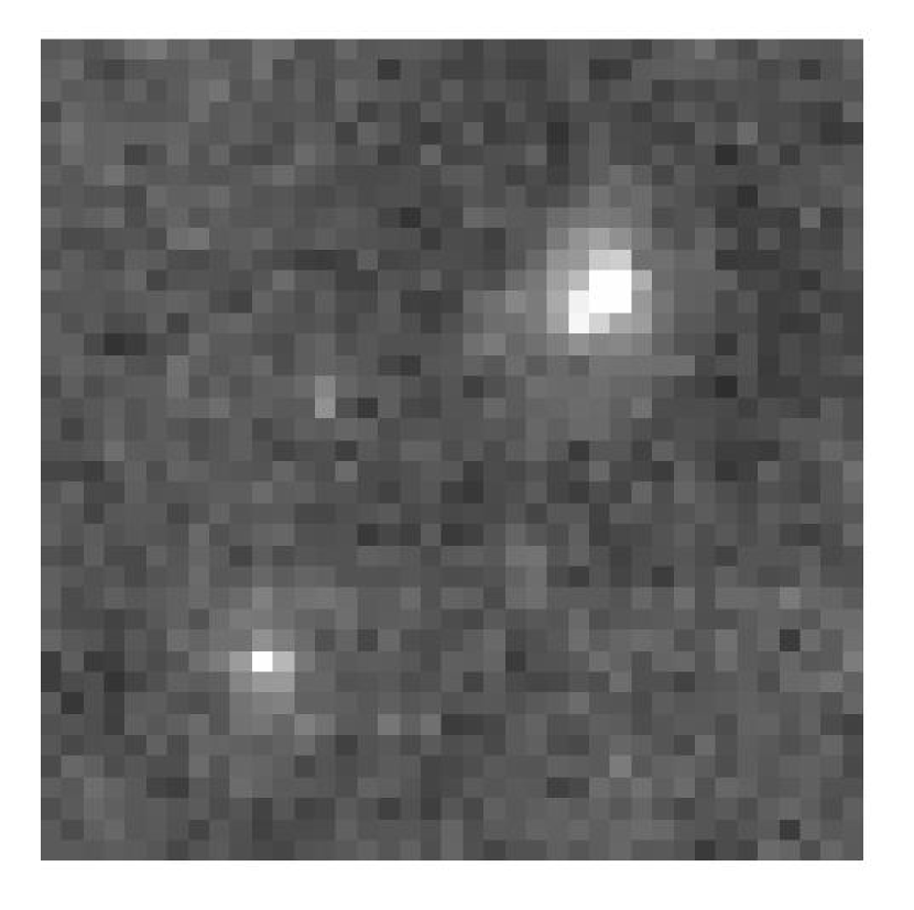
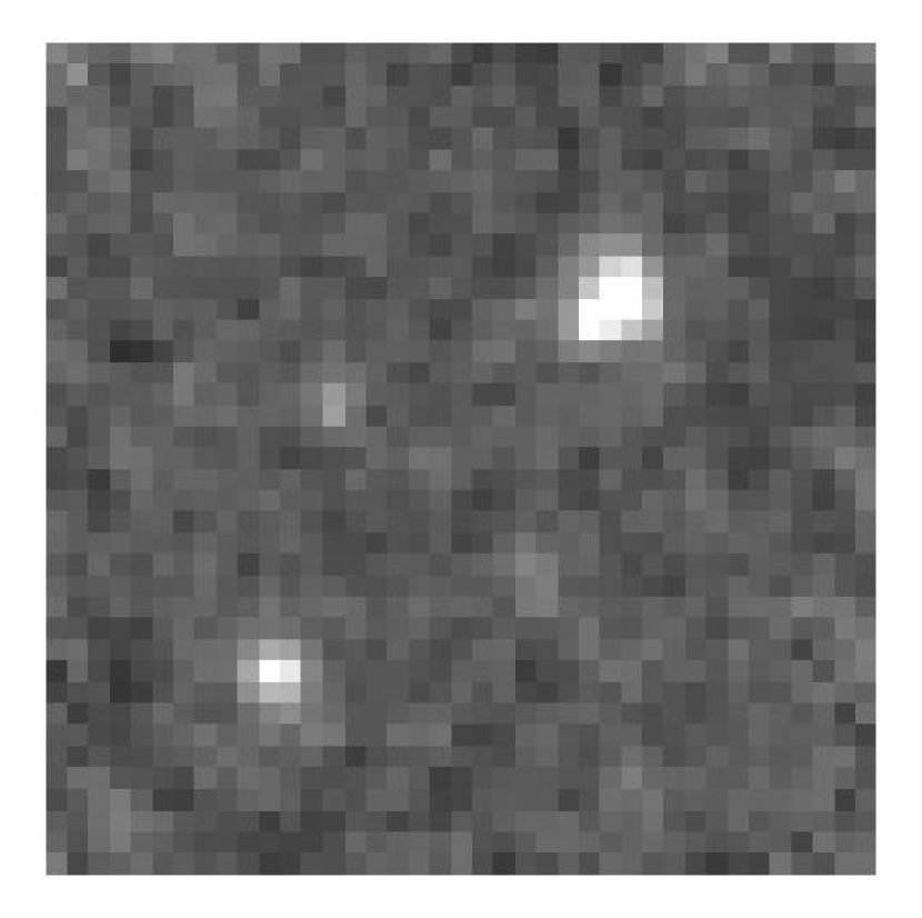
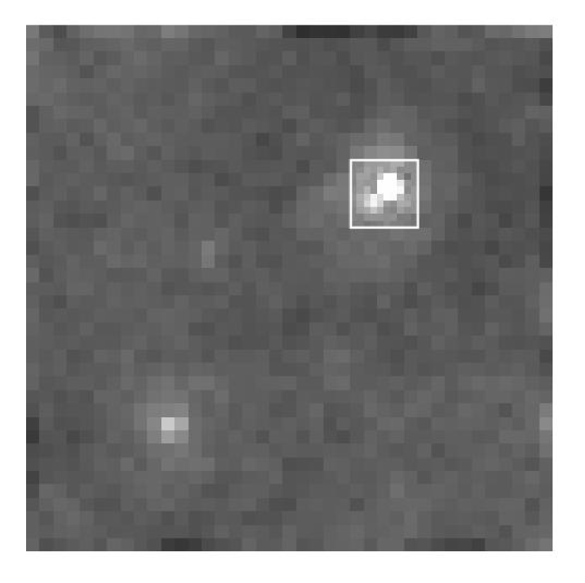
Figure 3: The input surface mass density of the five clusters listed in Table 1 (top left) and the single-resolution inverse reconstruction (top right), the direct reconstruction (bottom left) and the multi-resolution inverse reconstruction (bottom right) of the $1\deg^{2}$ simulated field. The resolution in the box around the first and second clusters in the multi-resolution map is $0^{\prime}.75$ per pixel whereas the resolution in the rest of the field is $1^{\prime}.5$ per pixel ($\sim$ 480 Kpc at $z=0.4$), which is also the resolution of the other maps.

Figure 7: The final multi-resolution convergence map of the $4\deg^{2}$ DLS F2. The resolution in the box around the A781 complex is $0^{\prime}.75$ per pixel whereas the resolution in the rest of the field is $1^{\prime}.5$ per pixel.

Table 1: Simulated NFW Clusters

Cluster	$x$ (pix)	$y$ (pix)	$r_{s}$ (Kpc)	$r_{200}$ (Mpc)	Mass ($10^{14}\times$ M☉)
1	10000.0	10000.0	430.13	2.151	26.1
2	9500.0	9500.	268.83	1.075	3.3
3	4000.0	3500.0	322.60	1.505	9.0
4	5000.0	8000.0	172.05	0.806	1.3
5	8250.0	5400.0	134.42	0.645	0.7

Note. — Properties of the simulated NFW clusters ($z=0.4$). The height and width of the field are 1 degree = 14400 pixels.

Table 2: Measured $\kappa_{\mathrm{total}}$ of Simulated Clusters

	Analytical Input			Inverse Method
Cluster	Position (pix)	$\kappa_{\mathrm{total}}$		Position (pix)	$\kappa_{\mathrm{total}}$	$P_{\mathrm{real}}$
1, 2	(26.76, 26.76)	5.310		(26.87, 27.43)	6.164 $\pm$ 0.360	99.97%
3	(11.03, 9.70)	1.510		(11.15, 9.66)	1.640 $\pm$ 0.273	99.95%
4	(13.76, 21.80)	0.308		(14.00, 22.44)	0.250 $\pm$ 0.129	84.83%
5	(22.22, 14.79)	0.170		(23.52, 15.00)	0.134 $\pm$ 0.096	72.62%

Note. — The measured total surface mass density of the simulated clusters from the analytical input and our inverse method, all shown in Figure 3. A mass sheet corresponding to the degeneracy coefficient of $\alpha\sim 0.88$ (Eqn. 1) transforms the measured surface mass density to the expected surface mass within the estimated errors. The error and probability estimates are derived from Monte Carlo simulations. The probability of finding objects in randomly selected regions of the Monte Carlo mass maps with the same or less signal than that of each cluster determines the probability of detecting such signal solely due to random orientation of background sources. One minus this probability is a fair estimate for the probability of detections to be real, $P_{\mathrm{real}}$.

References

- Bartelmann et al. (1996) Bartelmann, M., Narayan, R., Seitz, S. & Schneider, P. 1996, ApJ, 464, L115
- Beckwith (2005) Beckwith, S. 2004, Hubble Ultra Deep Field Catalog, (STScI), http://www.stsci.edu/hst/ud
- Bernstein & Jarvis (2002) Bernstein, G.M. & Jarvis, M. 2002, AJ, 123,583
- Bertin & Arnouts (1996) Bertin, E. & Arnouts, S. 1996, A&AS, 117, 393
- Bradac et al. (2005) Bradac, M., Schneider, P., Lombardi, M. & Erben, T. 2005, A&A, 437, 39
- Bridle et al. (1998) Bridle, S.L., Hobson, M.P., Lasenby, A.N. & Saunders, R. 1998, MNRAS, 299, 895
- Broadhurst et al. (1995) Broadhurst, T.J., Taylor, A. & Peacock, J. 1995, ApJ, 438, 49
- Fischer & Tyson (1997) Fischer, P. & Tyson, J.A. 1997, AJ, 114, 14
- Geller et al. (2005) Geller, M., Dell’Antonio, I., Kurtz, M., Ramella, M., Fabricant, D., Caldwell, N., Tyson, A. & Wittman, D. 2005, ApjL, 635, 125
- Jain et al. (2006) Jain, B., Jarvis, M. & Bernstein, G. 2006, JCAP, 0602, 001
- Kaiser & Squires (1993) Kaiser, N. & Squires, G. 1993, ApJ, 404, 441
- Lombard & Bertin (1999) Lombardi M. & Bertin G. 1999, A&A, 342, 337
- Marshall et al. (2002) Marshall, P.J., Hobson, M.P., Gull, S.F. & Bridle, S.L. 2002, MNRAS, 335, 1037
- Miralda-Escudé (1991) Miralda-Escudé, J. 1991, ApJ, 380, 1
- Navarro, Frenk & White (1997) Navarro, J.F., Frenk, C.S. & White, S.D.M. 1997, ApJ, 490, 493
- Parker et al. (2007) Parker, L.C., Hoekstra, H., Hudson, M.J., van Waerbeke, L. & Mellier, Y. 2007, ApJ, 669, 21P
- Press et al. (1992) Press, W.H., Teukolsky, S.A., Vetterling, W.T. & Flannery, B.P. 1992, Numerical Recipes in C, Cambridge (Cambridge University Press)
- Schneider & Seitz (1995) Schneider, P. & Seitz, C. 1995, A&A, 294, 411
- Sehgal et al. (2007) Sehgal, N., Hughes, J., Wittman, D., Margoniner, V., Tyson, J. A., Gee, P. & Dell’Antonio, I. 2007 ApJ, submitted
- Seitz et al. (1998) Seitz, C., Schneider, P. & Bartelmann, M. 1998, A&A, 337, 325
- Squires & Kaiser (1996) Squires, G. & Kaiser, N. 1996, 473, 65
- Tyson (1988) Tyson, J.A 1988, AJ, 98, 1
- Tyson et al. (1990) Tyson, J.A , Wenk, R.A. & Valdes, F.V. 1990 ApjL, 349, 1
- Wall & Jenkins (2003) Wall, J.V. & Jenkins, C.R. 2003, Practical Statistics for Astronomers, Cambridge (Cambridge University Press)
- Wittman et al. (2006) Wittman, D., Dell’Antonio, I.P., Hughes, J.P., Margoniner, V.E., Tyson, J.A., Cohen, J.G. & Norman, D. 2006, ApJ, 643, 128
- Wittman et al. (2002) Wittman, D., Tyson, J.A. & Dell’Antonio, I.P. 2002, Proc. SPIE, 4863, 73
- Wittman et al. (2000) Wittman, D.M., Tyson, J.A., Kirkman, D., Dell’Antonio, I.P. & Bernstein, G. 2000, Nature, 405, 143
- Wright & Brainerd (2000) Wright, C.O. & Brainerd, T.G. 2000, ApJ, 534, 34