The Szekeres Swiss Cheese model and the CMB observations

Abstract

This paper presents the application of the Szekeres Swiss Cheese model to the analysis of observations of the cosmic microwave background (CMB) radiation. The impact of inhomogeneous matter distribution on the CMB observations is in most cases studied within the linear perturbations of the Friedmann model. However, since the density contrast and the Weyl curvature within the cosmic structures are large, this issue is worth studying using another approach. The Szekeres model is an inhomogeneous, non-symmetrical and exact solution of the Einstein equations. In this model, light propagation and matter evolution can be exactly calculated, without such approximations as small amplitude of the density contrast. This allows to examine in more realistic manner the contribution of the light propagation effect to the measured CMB temperature fluctuations.

The results of such analysis show that small-scale, non-linear inhomogeneities induce, via Rees-Sciama effect, temperature fluctuations of amplitude $10^{-7}-10^{-5}$ on angular scale $\vartheta<0.24^{\circ}$ ($\ell>750$). This is still much smaller than the measured temperature fluctuations on this angular scale. However, local and uncompensated inhomogeneities can induce temperature fluctuations of amplitude as large as $10^{-3}$, and thus can be responsible the low multipoles anomalies observed in the angular CMB power spectrum.

1 Introduction

The Universe, as it is observed, is very inhomogeneous. Among structures observed in the Universe are clusters and superclusters of galaxies as well as large cosmic voids. This inhomogeneous matter distribution affects light propagation and hence astronomical observations. The study of light propagation effects is considerably important when analysing the CMB observations. This is because the last scattering surface is the most remote region which is observable using electromagnetic radiation. In standard approach the CMB temperature fluctuations are analysed by solving the Boltzmann equation within linear perturbations around the homogeneous and isotropic Friedmann–Lemaître–Robertson–Walker (FLRW) model SZ96 ; SSWZ03 . The application of the FLRW model as a background model results in a remarkably good fit to the CMB data H08 . However, the assumption of homogeneity, which is also consistent with other types of cosmological observations is not a direct consequence of them E08 . It is often said that such theorems like the Ehlers-Geren-Sachs theorem EGS and the ‘almost EGS theorem’ SME justify the application of the FLRW models. These theorems state that if anisotropies in the cosmic microwave background radiation are small for all fundamental observers then locally the Universe is almost spatially homogeneous and isotropic. However, as shown in NUWL99 , it is possible that the CMB temperature fluctuations are small but the Weyl curvature is large. In such a case the geometry of the Universe is far from the Robertson–Walker geometry and the applicability of FLRW models is not justified. Moreover, the applicability of the linear approach can be questionable since the density contrast within cosmic structures is much larger than unity. Therefore, there is a need for application of exact and inhomogeneous models to the study of the light propagation and its impact on the CMB temperature fluctuations. This issue has been extensively studied within spherically symmetric models — within the thin shell approximation TV87 ; IS06 ; IS07 and within the Lemaître–Tolman model P92 ; AFMS93 ; SAF93 ; AFS94 ; FSA94 ; RRS06 ; MN08 . However, most of the cosmic structures are not spherically symmetric, and thus the study of light propagation in non-spherical models is essential. One of the suitable models for this purpose is the Szekeres model. The Szekeres model has no symmetry, allows to study a nonlinear evolution and does not require small Weyl curvature. Therefore, this paper aims to study the CMB temperature fluctuations in the Swiss Cheese Szekeres model.

The structure of this paper is as follows. Sec. 2 presents basic formulae describing light propagation; in Sec. 3 the Szekeres model is presented; Sec. 4 presents the construction of models; Sec. 5 presents the findings.

2 Light propagation

Light propagates along null geodesics. If $k^{\alpha}$ is a vector tangent to a null geodesic, then

$$k_{\alpha}k^{\alpha}=0,\qquad k_{\alpha;\beta}k^{\beta}=0.$$ (1)

As light propagates, the frequency of photons changes. The ratio of the frequency of a photon at the emission event to the measured frequency defines the redshift

$$\frac{\nu_{e}}{\nu_{o}}:=1+z.$$ (2)

Since photon’s energy, as measured by an observer with the 4-velocity $u^{\alpha}$, is proportional to $k^{\alpha}u_{\alpha}$, thus the redshift obeys the following relation

$$1+z=\frac{\left(k^{\alpha}u_{\alpha}\right)_{e}}{\left(k^{\alpha}u_{\alpha}\right)_{o}},$$ (3)

where the subscripts _e and _o refer to instants of emission and observation respectively. Assuming that the black body spectrum is conserved, the temperature must be proportional to $1+z$

$$\frac{T_{e}}{T_{o}}=1+z.$$ (4)

Then, from eq. (4), the temperature fluctuations measured by co-moving observer are:

$$\left(\frac{\Delta T}{T}\right)_{o}=\frac{T_{e}/(1+z)-\bar{T}_{e}/(1+\bar{z})}{\bar{T}_{e}/(1+\bar{z})},$$ (5)

where quantities with bars $~{}\bar{}~{}$ refer to average quantities. If the temperature at the emission is $T_{e}=\bar{T}_{e}+\Delta T_{e}$, then

$$\left(\frac{\Delta T}{T}\right)_{o}=\frac{\bar{z}-z}{1+z}+\left(\frac{\Delta T}{\bar{T}}\right)_{e}\frac{1+\bar{z}}{1+z}.$$ (6)

As can be seen from the above formula, the observed temperature fluctuations on the CMB sky are caused by the light propagation effects and by the temperature fluctuations at the decoupling instant.

3 The Szekeres model

3.1 The metric of the Szekeres model

For our purpose it is convenient to use a coordinate system different from that in which Szekeres S75 originally found his solution. The metric is of the following form C96

$${\rm d}s^{2}=c^{2}{\rm d}t^{2}-\frac{(\Phi,_{r}-\Phi E,_{r}/E)^{2}}{(\varepsilon-k)}{\rm d}r^{2}-\Phi^{2}\frac{({\rm d}p^{2}+{\rm d}q^{2})}{E^{2}},$$ (7)

where $\Phi$ is a function of $t$ and $r$, $\varepsilon=\pm 1,0$ and $k=k(r)\leq\varepsilon$ is an arbitrary function of $r$. The function $E$ is given by

$$E(r,p,q)=\frac{1}{2S}(p^{2}+q^{2})-\frac{P}{S}p-\frac{Q}{S}q+C,$$ (8)

where the functions $S=S(r)$, $P=P(r)$, $Q=Q(r)$, and $C=C(r)$ satisfy the relation

$$C=\frac{P^{2}}{2S}+\frac{Q^{2}}{2S}+\frac{S}{2}\varepsilon,~{}~{}~{}~{}~{}~{}~{}~{}~{}\varepsilon=0,\pm 1.$$ (9)

Originally, Szekeres considered only a case of $p=0=\Lambda$. This result was generalised by Szafron Szf77 to the case of uniform pressure, $p=p(t)$. A spacial case of this solution, the cosmological constant, was in detailed discussed by Barrow and Stein-Schabes BSS84 .

The $\varepsilon=-1$ case is often called the quasihyperbolic Szekeres model (for a detailed discussion on the quasihyperbolic Szekeres models see HK08 ), $\varepsilon=0$ quasiplane (for details see HK08 ; K08 ), and $\varepsilon=1$ quasispherical (for details see HK02 ). Although it is possible to have within one model quasispherical and quasihyperbolic regions separated by the quasiplane regions HK08 , only the quasispherial case will be considered here.

In the quasispherial case surfaces of constant $t$ and $r$ are spheres. The transformation from ($p,q$) coordinates into ($\vartheta$, $\varphi$) coordinates is HK02

$$p=S\cot\frac{\vartheta}{2}\cos\varphi+P,$$

$$q=S\cot\frac{\vartheta}{2}\sin\varphi+Q.$$ (10)

3.2 The Einstein equations

Applying metric (7) to the Einstein equations, and assuming the energy momentum tensor for a dust, the Einstein equations reduce to the following two

$$\frac{1}{c^{2}}\Phi,_{t}^{2}=\frac{2M}{\Phi}-k+\frac{1}{3}\Lambda\Phi^{2},$$ (11)

$$4\pi\frac{G}{c^{2}}\rho=\frac{M,_{r}-3ME,_{r}/E}{\Phi^{2}(\Phi,_{r}-\Phi E,_{r}/E)}.$$ (12)

where $\rho$ is matter energy density, $M(r)$ is another function of radial coordinate. In a Newtonian limit $Mc^{2}/G$ is equal to the mass inside the shell of radial coordinate $r$. However, it is not an integrated rest mass but active gravitational mass that generates a gravitational field.

Eq. (11) can be integrated

$$\int\limits_{0}^{\Phi}\frac{{\rm d}\tilde{\Phi}}{\sqrt{\frac{2M}{\tilde{\Phi}}-k+\frac{1}{3}\Lambda\tilde{\Phi}^{2}}}=c(t-t_{B}),$$ (13)

where $t_{B}(r)$ is an arbitrary function of $r$. This means that the big bang is not a single event as in the FLRW models but occurs at different times for different distances from the origin.

As can be seen the Szekeres model is specified by 6 functions. However, by a choice of the appropriate coordinates, the number of independent functions can be reduced to 5.

3.3 General properties and the Friedmann limit

The vorticity within the Szekeres model is zero. In addition the acceleration vanishes, $u^{\alpha}{};_{\beta}u^{\beta}=0$. The shear tensor is

$$\sigma^{\alpha}{}_{\beta}=\frac{1}{3}\left(\frac{\Phi,_{tr}-\Phi,_{t}\Phi,_{r}/\Phi}{\Phi,_{r}-\Phi E,_{r}/E}\right){\rm diag}(0,2,-1,-1).$$ (14)

The scalar of expansion is

$$\theta=u^{\alpha}{}_{;\alpha}=\frac{\Phi,_{tr}+2\Phi,_{t}\Phi,_{r}/\Phi-3\Phi,_{t}E,_{r}/E}{\Phi,_{r}-\Phi E,_{r}/E}.$$ (15)

The Weyl curvature decomposed into its electric and magnetic part is of the following form

$$E^{\alpha}{}_{\beta}=C^{\alpha}{}_{\gamma\beta\delta}u^{\gamma}u^{\delta}=\frac{M(3\Phi,_{r}-\Phi M,_{r}/M)}{3\Phi^{3}(\Phi,_{r}-\Phi E,_{r}/E)}{\rm diag}(0,2,-1,-1),$$

$$H_{\alpha\beta}=\frac{1}{2}\sqrt{-g}\rho_{\alpha\gamma\mu\nu}C^{\mu\nu}{}_{\beta\delta}u^{\gamma}u^{\delta}=0.$$ (16)

Finally, the 4D and 3D Ricci scalars are

$${}^{4}\mathcal{R}=-\kappa\rho c^{2}-4\Lambda,$$

$${}^{3}\mathcal{R}=2\frac{k}{\Phi^{2}}\left(\frac{\Phi k,_{r}/k-2\Phi E,_{r}/E}{\Phi,_{r}-\Phi E,_{r}/E}+1\right).$$ (17)

In the Friedmann limit, $\Phi\rightarrow ra_{F}$, $k\rightarrow k_{F}r^{2}$ and $M\rightarrow M_{F}r^{3}$ where $a_{F}$ is the Friedmann scale factor, $k_{F}$ is the curvature index and is a constant, and $M_{F}$ is another constant. As can be seen in Friedmann limit:

$$\theta \rightarrow 3\frac{a_{F},_{t}}{a_{F}},$$ (18)

$$\sigma^{\alpha}{}_{\beta} \rightarrow 0,$$

$$E^{\alpha}{}_{\beta} \rightarrow 0,$$

$${}^{4}\mathcal{R} \rightarrow-6\frac{M_{F}}{a_{F}^{3}}-4\Lambda,$$

$${}^{3}\mathcal{R} \rightarrow 6\frac{k_{F}}{a_{F}^{2}}.$$

3.4 Null geodesic equations

The geodesic equations

$$\frac{{\rm d}^{2}x^{\alpha}}{{\rm d}s^{2}}+\Gamma^{\alpha}_{\beta\gamma}\frac{{\rm d}x^{\beta}}{{\rm d}s}\frac{{\rm d}x^{\gamma}}{{\rm d}s}=0.$$ (19)

in the quasispherical Szekeres model, are of the following form

$\alpha=0$:

$$\frac{{\rm d}^{2}t}{{\rm d}s^{2}}+\frac{{\Phi,_{tr}}-{\Phi,_{t}}{E},_{r}/E}{1-k}(\Phi,_{r}-\Phi E,_{r}/E)\left(\frac{{\rm d}r}{{\rm d}s}\right)^{2}$$

$$+\frac{\Phi{\Phi,_{t}}}{E^{2}}\left[\left(\frac{{\rm d}p}{{\rm d}s}\right)^{2}+\left(\frac{{\rm d}q}{{\rm d}s}\right)^{2}\right]=0,$$ (20)

$\alpha=1$:

$$\frac{{\rm d}^{2}r}{{\rm d}s^{2}}+2\frac{{\Phi,_{tr}}-{\Phi,_{t}}{E},_{r}/E}{\Phi,_{r}-\Phi E,_{r}/E}\frac{{\rm d}t}{{\rm d}s}\frac{{\rm d}r}{{\rm d}s}-\frac{\Phi}{E^{2}}\frac{1-k}{\Phi,_{r}-\Phi E,_{r}/E}\left[\left(\frac{{\rm d}p}{{\rm d}s}\right)^{2}+\left(\frac{{\rm d}q}{{\rm d}s}\right)^{2}\right]$$

$$+\left[\frac{\Phi,_{rr}-\Phi,_{r}E,_{r}/E-\Phi{E},_{rr}/E+\Phi(E,_{r}/E)^{2}}{\Phi,_{r}-\Phi{E},_{r}/E}+\frac{1}{2}\frac{k,_{r}}{1-k}\right]\left(\frac{{\rm d}r}{{\rm d}s}\right)^{2}$$

$$+2\frac{\Phi}{E^{2}}\frac{E,_{r}E,_{p}-EE,_{pr}}{\Phi,_{r}-\Phi E,_{r}/E}\frac{{\rm d}r}{{\rm d}s}\frac{{\rm d}p}{{\rm d}s}+2\frac{\Phi}{E^{2}}\frac{(E,_{r}E,_{q}-E{E},_{qr})}{\Phi,_{r}-\Phi E,_{r}/E}\frac{{\rm d}r}{{\rm d}s}\frac{{\rm d}q}{{\rm d}s}=0,$$ (21)

$\alpha=2$:

$$\frac{{\rm d}^{2}p}{{\rm d}s^{2}}+2\frac{{\Phi,_{t}}}{\Phi}\frac{{\rm d}t}{{\rm d}s}\frac{{\rm d}p}{{\rm d}s}-\left[\frac{{\Phi},_{r}-{\Phi}E,_{r}/E}{\Phi(1-k)}(E,_{r}E,_{p}-{E}E,_{pr})\right]\left(\frac{{\rm d}r}{{\rm d}s}\right)^{2}+\frac{E,_{p}}{E}\left(\frac{{\rm d}q}{{\rm d}s}\right)^{2}$$

$$+2\left(\frac{\Phi,_{r}}{\Phi}-\frac{E,_{r}}{E}\right)\frac{{\rm d}r}{{\rm d}s}\frac{{\rm d}p}{{\rm d}s}-\frac{E,_{p}}{E}\left(\frac{{\rm d}p}{{\rm d}s}\right)^{2}-2\frac{E,_{q}}{E}\frac{{\rm d}p}{{\rm d}s}\frac{{\rm d}q}{{\rm d}s}=0,$$ (22)

$\alpha=3$:

$$\frac{{\rm d}^{2}q}{{\rm d}s^{2}}+2\frac{{\Phi,_{t}}}{\Phi}\frac{{\rm d}t}{{\rm d}s}\frac{{\rm d}q}{{\rm d}s}-\left[\frac{\Phi,_{r}-{\Phi}E,_{r}/E}{\Phi(1-k)}(E,_{r}E,_{q}-{E}E,_{qr})\right]\left(\frac{{\rm d}r}{{\rm d}s}\right)^{2}-\frac{E,_{q}}{E}\left(\frac{{\rm d}q}{{\rm d}s}\right)^{2}$$

$$+2\left(\frac{\Phi,_{r}}{\Phi}-\frac{E,_{r}}{E}\right)\frac{{\rm d}r}{{\rm d}s}\frac{{\rm d}q}{{\rm d}s}+\frac{{E},_{q}}{E}\left(\frac{{\rm d}p}{{\rm d}s}\right)^{2}-2\frac{{E},_{p}}{E}\frac{{\rm d}p}{{\rm d}s}\frac{{\rm d}q}{{\rm d}s}=0.$$ (23)

Equations (20) – (23) are quite complicated. However, if two coordinates could be constant on a geodesic, then we could impose ${\rm d}p={\rm d}q=0$ on a general solution of (7) to get

$$\frac{{\rm d}t}{{\rm d}r}=\pm\frac{\Phi,_{r}-\Phi E,_{r}/E}{\sqrt{1-k}},$$ (24)

where $+$ is for outwards directed geodesics and $-$ for inwards directed geodesics. In such a case the redshift formula (3) would reduce to the much simpler form (see Appendix A for derivation)

$$\ln(1+z)=\pm\int\limits_{r_{e}}^{r_{o}}{\rm d}r\frac{\Phi,_{tr}-\Phi,_{t}E,_{r}/E}{\sqrt{1-k}}.$$ (25)

Thus, if such fixed-direction geodesics exist, then the study of light propagation in the Szekeres model could be significantly simplified. Instead of solving eqs. (20) – (23) only eq. (24) would have to be solved to find a null geodesic and only eq. (25) to find the redshift. However, in general ${\rm d}^{2}p/{\rm d}s^{2}\neq 0$ and ${\rm d}^{2}q/{\rm d}s^{2}\neq 0$, i.e. the condition ${\rm d}p={\rm d}q=0$ cannot hold along the null geodesic. As follows from (20) – (23) if initially $k^{p}=k^{q}=0$, then the coordinates $p$ and $q$ will remain constant only if along the whole geodesic

$$\Phi,_{r}=\Phi\frac{E,_{r}}{E},$$ (26)

or

$$EE,_{pr}=E,_{p}E,_{r}~{}~{}~{}{\rm and}~{}~{}~{}EE,_{qr}=E,_{q}E,_{r}.$$ (27)

The relation (26) holds only at a shell crossing singularity which must be eliminated in a physically acceptable model. Apart from the spherical symmetry (i.e. the Lemaître–Tolman model) the relations (27) hold only in the axially symmetric case ND07 . It should be noted that not every Szekeres model is axially symmetric. Moreover, apart from the spherical symmetry there is only one such geodesic, which propagates along the symmetry axis. Thus, such a geodesic will be referred to as the axial geodesics.

4 The Swiss Cheese model

4.1 Arrangement of the Swiss Cheese model

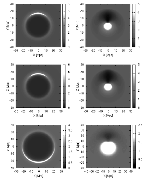
Figure 1: The density distribution, $\rho/\rho_{b}$, at the current instant for regions A (upper left), B (upper right), C (middle left), D (middle right), E (lower left) and F (lower right). In regions A, B, E and F the dipole axis is aligned with the Y axis. For these regions the density distribution is presented for the surface $Z=0$. In regions C and D the dipole is aligned with the Z axis. For these regions the density distribution is presented for the surface $Y=0$. Coordinates $X,Y,Z$ are defined as $X=\Phi\cos\varphi\sin\vartheta,Y=\Phi\sin\varphi\sin\vartheta,Z=\Phi\cos\vartheta$ [where $\vartheta$ and $\varphi$ are given by (10)]. The exact forms of functions used to specify these models are included in Appendix B.

The Swiss Cheese models which are employed in this paper are constructed from six different building blocks – regions A-F (holes) – which are matched with the Friedmann background (cheese). These Szekeres patches are placed so that their boundaries touch wherever a light ray exits one inhomogeneous patch. Thus the ray immediately enters another Szekeres inhomogeneity and does not spend any time in the Friedmann background. Using different sequences of regions A – F five models are constructed, . The density distribution at the current instant within each of these regions is presented in Fig. 1. The exact forms of functions used to specify the Szekeres model in each of these regions are presented in Appendix B. As can be seen from the detailed specification (Appendix B) the functions defining regions A–D become for the radial cooridate $r\geqslant 24$ kpc of exactly the same form as the form in the Friedmann background [compare the form of the functions in Appendix B with the form of functions in the Friedmann limit, eqs. (18)]. Regions E and F tend exponentially to the Friedmann models. However, as seen from their specification or from Fig. 2, at the distance $r\approx 30$ kpc and $r\approx 40$ kpc, respectively, regions E and F become almost Friedmann. Figure 2 presents the curvature scalar, ${\mathcal{W}}^{2}$, which is defined as

$$\mathcal{W}^{2}=\frac{E_{\alpha\beta}E^{\alpha\beta}}{6H^{4}},$$ (28)

where $E_{\alpha\beta}$ is the electric part of the Weyl tensor (3.3) and $H=(1/3)\theta$ is the Hubble parameter (15). As can be seen, in some regions ${\mathcal{W}}^{2}\gg 1$. This feature, apart from nonlinear evolution and non-symmetrical shape, makes the application of the Szekeres model more realistic.

4.2 Junction conditions

When constructing a Swiss Cheese model, we need to satisfy the junction conditions for matching the particular inhomogeneous patches to the Friedmann background, and also assure the continuity of the null geodesics. The standard junction conditions are that the 3D-metric of the surface and its extrinsic curvature, the first and second fundamental forms, must be continuous.

For matching a Szekeres patch to a Friedmann background across a comoving spherical surface, $r=$ constant, the conditions are: that the mass inside the junction surface in the Szekeres patch is equal to the mass that would be inside that surface in the homogeneous background; that the spatial curvature at the junction surface is the same in both the Szekeres and Friedmann models, which implies that $k_{SZ}=k_{F}r^{2}$ and $(k_{SZ}),_{r}=2k_{F}r$; finally that the bang time and also $\Lambda$ must be continuous across the junction. The mass $M$ and the curvature function $k$ are matched by the construction — see Appendix B. The value of the cosmological constant is the same in all regions, and the value of the bang time function is fixed by (13), and at the junction is equal to $t_{B}=0$. It might be surprising that a non-symmetrical model like the Szekeres can be joined with the symmetric FLRW model, but there are other examples of such junctions. For example Bonnor demonstrated that the Szekeres model can be matched to the Schwarzschild solution B76 .

The junction of null geodesics requires the continuity of all components of the null vector. However, let us notice that when one Szekeres sphere is matched to another Szekeres sphere it can be rotated around the normal direction. Thus, we only need to match up the time component, $k^{0}$ and the tangential component. The tangential component is defined as

$$k^{T}=\frac{\Phi}{E}\sqrt{(k^{p})^{2}+(k^{q})^{2}}.$$ (29)

The radial component is then given by the null condition, $k_{\alpha}k^{\alpha}=0$.

Figure 2: The Weyl curvature scalar ${\mathcal{W}}^{2}$ [eq. (3.3)] evaluated at the current instant, along the dipole axis, R, in Szekeres regions A–F (for regions A, B, D, and E, R =Y, for regions C and D, R=X). The 3D shape of these profiles is very similar to the shape of the density distribution – see Fig. 1. Since the FLRW models are conformally flat, the Szekeres regions are in some parts far from being even a close (linear) approximation of the FLRW model.

4.3 Description of models

Five different Szekeres Swiss Cheeses models are considered here:

1. Model 1

   Model 1 is constructed from alternately matching regions A and B (A + B + A + B …) into the Friedmann background. When a light ray exits one Szekeres region, it immediately enters another inhomogeneous patch. Each time the $(p,q)$ position of the point of entry is randomly selected. In addition $k^{p}$ and $k^{q}$ are quasi-randomly selected, i.e

   $$(k^{q})^{2}=\gamma\left(k^{T}\frac{E}{\Phi}\right)^{2},\quad(k^{p})^{2}=(1-\gamma)\left(k^{T}\frac{E}{\Phi}\right)^{2},$$

   where $\gamma$ is a random value in the range $0\leqslant\gamma\leqslant 1$. The radial coordinate of the matching point is $r_{j}=24$ kpc – the point where the Szekeres region becomes Friedmann.

2. Model 2

   This model is constructed from alternating regions C and D, but only axial null geodesics are considered, i.e.  $k^{p}=0$ and $k^{q}=0$, $p=q=0$. The radial component of the matching point is again $r_{j}=24$ kpc.

3. Model 3

   The next model consists of regions E and F placed alternately. Null vector components $k^{p}$ and $k^{q}$ are chosen in such a way that $10^{-8}\leqslant k^{p}\leqslant 10^{-4}$ and $10^{-8}\leqslant k^{q}\leqslant 10^{-4}$, but are otherwise random. As can be noted, this is not in accordance with condition (29). In order to maintain the continuity of the tangential component of the null vector the next Szekeres patch must by reoriented with respect to the preceding patch. This however leads to an overlapping of these two Szekeres regions. Although, at the junction point ($r_{j}=40$ kpc for region E, and $r_{j}=50$ kpc for region F), these two regions are almost Friedmann, still this is not a perfect matching. We proceed with this type of imperfect matching to study how randomly chosen values of the tangential component (hence more randomised light propagation through a Szekeres patch) influences the final results.

4. Model 4

   Model 4 is constructed using only C regions, with $r_{j}=24$ kpc, and only axial geodesics are considered, i.e. $k^{p}=k^{q}=p=q=0$.

5. Model 5

   The last model is also axially symmetric, $k^{p}=k^{q}=p=q=0$, $r_{j}=24$ kpc, but uses only D regions.

5 Results

5.1 The Rees-Sciama effect

Figure 3: The temperature fluctuations caused by light propagation effects in models 1-5. In models 1-3 light propagates alternatively though underdense and overdense regions. In model 4 light propagates only though regions of $\delta M<0,\delta k>0$, and in model 5 only through regions of $\delta M>0,\delta k<0$ (see Sec. 4 for a detail description on how these models were constructed).

Figure 4: A small part of the light propagation in model 3. The left panel shows the density variation that light ‘feels’ as it propagates. The black thin dotted line shows the density in the background model. The right panel presents the temperature fluctuations as measured by an observer situated outside the structure in the homogeneous FLRW region. The letters in the left and right panels label corresponding points along the light path.

To estimate the temperature fluctuations induced by the light propagation effects, it is assumed that initial temperature distribution is uniform, $(\Delta T/T)_{e}=0$. Then temperature fluctuations are calculated using (LABEL:7.3), and they are plotted against time of propagation in Fig. 3. As seen, the final values are small, of amplitude $\Delta T/T\approx 10^{-7}$ (model 3), $\Delta T/T\approx 10^{-6}$ (models 1 and 2), and $\Delta T/T\approx 10^{-5}$ (models 4 and 5). A detailed analysis of how inhomogeneities induce temperature fluctuations is presented in Fig. 4 (for clarity, only a small fraction of the time is presented). The left panel of Fig. 4 shows the density of regions through which the light propagates in model 3. The right panel presents the temperature fluctuations as measured by an observer situated at the junction point where the model is that of Friedmann. Letters correspond to each inhomogeneous patch (left panel) and temperature fluctuations caused by them (right panel). Clearly, underdense regions induce negative temperature fluctuations, overdense regions induce positive fluctuations.

Apart from estimating the amplitude of the Rees–Sciama effect, it is also important to estimate the angular scale which is the most affected by this effect. Without going into any complicated analysis, we can estimate the angular scale by employing the following approximation: the correlation between two distant points on the sky is zero – photons which were propagating along two distant paths have the temperature fluctuations uncorrelated. Only when the light paths are near to each other are the temperature fluctuations correlated. Thus the simplest estimation of the angular scale of the Rees–Sciama effect, as seen from the schematic Fig. 5, is the angular size of the Szekeres patch at the last scattering instant. For the models studied in this section, such approximations lead to an angular scale of $\vartheta\approx 0.21^{\circ}$, or alternatively $\ell\approx 850$. If the photons are propagating along neighbouring paths for only half of the age of the Universe (in such a case, as seen from Fig. 6, the final temperature fluctuations are two times smaller), then the angular scale is similar, $\vartheta\approx 0.24^{\circ}$ ($\ell\approx 750$). Thus, the Rees–Sciama effect of amplitude $\sim 10^{-6}$ contributes to the CMB temperature fluctuations on the angular scale $\vartheta<0.25^{\circ}$ ($\ell>700$). This angular scale corresponds to the angular scale at which the third peak of the CMB angular power spectrum is observed. At this scale the measured rms temperature fluctuations are of amplitude $\approx 5\times 10^{-5}$. This is still several times higher than the results obtained within models 4 and 5. In the case of models 1–3 the measured value is more than one order of magnitude larger than the model estimates.

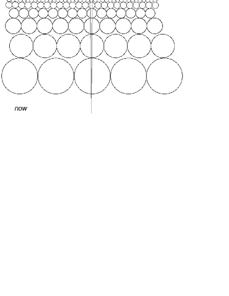
Figure 5: The schematic representation of the Swiss Cheese model. When two photons are propagating along a similar path the final temperature fluctuations are similar. If paths are different, then the final temperature fluctuations are also different and hence not correlated.

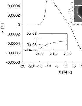
Figure 6: Temperature fluctuation amplitude, as measured by observers at different locations in region E, along the path of a light ray. The ray path is shown as the bright line in the upper inset.

5.2 The role of local structures

So far, it has been assumed that each inhomogeneous structure is compensated (i.e. each Szekeres region was matched with the FLRW background), and that measurements are carried out away from the inhomogeneities, i.e. where the universe is homogeneous. However in the real Universe there is no place where the cosmic structures in the observer’s vicinity are fully compensated and therefore the Universe should not be treated locally as homogeneous. Since all measurements are always local, let us consider what happens if temperature fluctuations are measured in an uncompensated region. Figure 6 presents the temperature fluctuations measured by an observer situated at different places within region E. These results are obtained under the assumption that light from last scattering is propagating through homogeneous regions, and currently reaches an observer in an inhomogeneous structure (region E). The light enters and propagates along the bright line shown in the upper right inset of Fig. 6. The above results show that local structures can significantly contribute to the CMB temperature fluctuations. This indicates that care must be exercised when extracting information from the CMB observations. Although it is highly unlikely that the signal caused by the local structures have a signature of acoustic oscillations we should be aware that local structures can have some visible impact on observations. Thus, it is important to test if local structures can cause the observed correlations of the alignment of dipole, quadrupole and octopole axes of angular power spectrum of the CMB temperature fluctuations (cf. SSHC ; LaM1 ; LaM2 ; Vale ; RRS ; RaSch ) or their low amplitude (cf. PP90 ; LP96 ; SC99 ).

6 Conclusions

The analysis presented in this paper has aimed to examine the influence of the light propagation effects on the temperature fluctuations of the CMB. The results indicate that the Rees-Sciama effect caused by the propagation of light through inhomogeneous but compensated structures do not significantly affect the CMB temperature fluctuations. Some would say that this is an obvious result since similar conclusion is reached when using perturbative methods. However, as it was argued in the Sec. 1, within real cosmic structures the density contrast and the Weyl curvature are significantly large. Thus, the application of the perturbation methods cannot be justified. It was shown, in this paper, that even in such cases light propagation effects are small. It has also been shown that the Rees–Sciama effect of amplitude $\sim 10^{-6}$ contributes to the CMB temperature fluctuations on the angular scale $\vartheta<0.25^{\circ}$ ($\ell>700$).

However, if the structures are not compensated or the measurements are carried out inside inhomogeneous non-compensated structures, the amplitude of measured temperature fluctuations can be slightly higher. Since in reality we cannot separate ourselves from the surroundings and say that all local structures at our positing are “compensated”, thus the local cosmic structures must be taken into account when analysing CMB observations. Especially, it is possible that the local structures can have some impact on low multipoles anomalies of the angular CMB power spectrum.

Appendix A The redshift formula for axial geodesics

To find a simplified redshift formula for the axial geodesics first we have to find $k^{0}$ in an affine parametrisation and then use the relation (3). Since we assume that $k^{2}=k^{3}=0$ then let us choose

$$k^{1}=-1,~{}~{}~{}~{}~{}~{}~{}~{}k^{0}=\frac{\Phi,_{r}-\Phi E,_{r}/E}{\sqrt{1-k}}.$$ (30)

The above parametrisation is not affine, thus the parallel transport does not preserve the tangent vector. Therefore $k^{\alpha}$, after being parallely transported, becomes $\lambda k^{\alpha}$ (where $\lambda$ is a scalar coefficient – a function of the parameter $s$ along the geodesic). In this case the geodesic equations are of form PK06

$$k^{\alpha};_{\beta}k^{\beta}=-\frac{1}{\lambda}\frac{{\rm d}\lambda}{{\rm d}s}k^{\alpha},$$ (31)

and reduce to

$$-\frac{1}{\lambda}\frac{{\rm d}\lambda}{{\rm d}s}=-\frac{\Phi,_{rr}-\Phi,_{r}E,_{r}/E-\Phi E,_{rr}/E+\Phi(E,_{r}/E)^{2}}{\Phi,_{r}-\Phi E,_{r}/E}$$

$$+2\frac{{\Phi},_{tr}-\Phi,_{t}E,_{r}/E}{\sqrt{1-k}}-\frac{k,_{r}}{2(1-k)}.$$ (32)

All the quantities above are evaluated on the null geodesic. In order to better depict which quantity is evaluated on the null geodesic a symbol $~{}\hat{}~{}$ is be used. Since on the geodesic $t$ and $r$ are connected with each other via relation (24), we have

$$\Phi_{n},_{r}=(\Phi,_{t})_{n}\frac{{\rm d}t}{{\rm d}r}+(\Phi,_{r})_{n}$$

$$(\Phi,_{r})_{n},_{r}=(\Phi,_{tr})_{n}\frac{{\rm d}t}{{\rm d}r}+(\Phi,_{rr})_{n},$$ (33)

where the subscript $n$ referees to quantities measured on the geodesic.

The second term in equation (32) looks like a logarithmic derivative. However because of (33) we have

$$\frac{{\rm d}\ln\left[(\Phi,_{r})_{n}-\Phi_{n}(E,_{r}/E)_{n}\right]}{{\rm d}r}=$$

$$\frac{(\Phi,_{r})_{n},_{r}-\Phi_{n},_{r}(E,_{r}/E)_{n}-\Phi_{n}({E},_{rr}/E)_{n}+\Phi_{n}(E,_{r}/E)^{2}_{n}}{(\Phi,_{r})_{n}-\Phi_{n}(E,_{r}/E)_{n}}=$$

$$\frac{(\Phi,_{rr})_{n}-(\Phi,_{r})_{n}(E,_{r}/E)_{n}-\Phi_{n}({E},_{rr}/E)_{n}+\Phi_{n}(E,_{r}/E)^{2}_{n}}{(\Phi,_{r})_{n}-\Phi_{n}(E,_{r}/E)_{n}}$$

$$+\frac{(\Phi,_{tr})_{n}-(\Phi,_{t})_{n}(E,_{r}/E)_{n}}{(\Phi,_{r})_{n}-\Phi_{n}(E,_{r}/E)_{n}}\frac{{\rm d}t}{{\rm d}r}.$$ (34)

Using the above relation we can integrate equation (32)

$$\lambda=C\frac{\sqrt{1-k}}{(\Phi,_{r})_{n}-\Phi_{n}(E,_{r}/{E})_{n}}~{}\exp\left(\int{\rm d}r\frac{(\Phi,_{tr})_{n}-(\Phi,_{t})_{n}({E},_{r}/E)_{n}}{\sqrt{1-k_{n}}}.\right)$$ (35)

Now we can easily find that $k^{\alpha}$ in the affine parametrisation is given by ${\tilde{k}}^{\alpha}=(\lambda/C)k^{\alpha}$. Using (3) we obtain

$$\ln(1+z)=\pm\int\limits_{r_{e}}^{r_{o}}{\rm d}r\frac{(\Phi,_{tr})_{n}-(\Phi,_{t})_{n}(E,_{r}/E)_{n}}{\sqrt{1-k_{n}}},$$ (36)

where $+$ is for ${r_{e}}<{r_{o}}$ and $-$ for ${r_{e}}>{r_{o}}$. Alternatively the redshift can be found by integration over time:

$$\ln(1+z)=\int\limits_{t_{e}}^{t_{o}}{\rm d}t\frac{(\Phi,_{tr})_{n}-(\Phi,_{t})_{n}(E,_{r}/E)_{n}}{(\Phi,_{r})_{n}-\Phi_{n}(E_{r}/E)_{n}}.$$ (37)

Appendix B Model specification and evaluation

In order to define the Szekeres model five functions of radial coordinate needed to be specified. In this paper all models will be defined by the following set of functions: $k,~{}M,~{}S,~{}P,$ and $Q$.

The algorithm used in the calculations can be defined as follows:

1. The radial coordinate is chosen to be the areal radius at the last scattering instant $r^{\prime}=\Phi(r,t_{LS})$. However, for clarity in further use, the prim is omitted and the new radial coordinate will be referred to as $r$.

2. The chosen background model is the $\Lambda$CDM model, i.e. a flat FLRW model with $\Lambda\neq 0$. The background density at the current instant is then given by

   $$\rho_{b}=\Omega_{m}\times\rho_{cr}=0.27\times\frac{3H_{0}^{2}}{8\pi G}.$$ (38)

   where the Hubble constant is $H_{0}=72$ km s^-1 Mpc^-1. The cosmological constant, $\Lambda$, corresponds to $\Omega_{\Lambda}=0.73$, where $\Omega_{\Lambda}=(1/3)(c^{2}\Lambda/H_{0}^{2})$.

3. The initial time, $t_{i}$, is chosen to be the time of last scattering, and is calculated from the following formula for a background FLRW universe P80

   $$t(z)=\frac{1}{H_{0}}\int\limits_{z}^{\infty}\frac{{\rm d}\tilde{z}}{(1+\tilde{z})\sqrt{\mathcal{D}(\tilde{z})}},$$ (39)

   where:

   $$\mathcal{D}(z)=\Omega_{m}(1+z)^{3}+\Omega_{K}(1+z)^{2}+\Omega_{\Lambda},$$ (40)

   where $\Omega_{K}=1-\Omega_{m}-\Omega_{\Lambda}$. For the lower limit of integration, $z=1089$ was used as the redshift at last scattering.

4. Six different Szekeres regions are considered in this paper. Let us denote them as regions A, B, C, D, E and F. The functions $M,~{}k,~{}Q,~{}P$ and $S$ in these regions are defined as follows

   • regions A and B

     $$M=M_{b}+\left\{\begin{array}[]{ll}M_{1}r^{3}&{\rm~{}for~{}}r\leqslant 0.5a,\\ M_{2}\exp\left[-12\left(\frac{r-a}{a}\right)^{2}\right]&{\rm~{}for~{}}0.5a\leqslant r\leqslant 1.5a\\ M_{1}(2a-r)^{3}&{\rm~{}for~{}}1.5a\leqslant r\leqslant 2a,\\ 0&{\rm~{}for~{}}r\geqslant 2a,\end{array}\right.$$

     where $M_{b}$ is the mass in the corresponding volume of the homogeneous universe, i.e. $M_{b}=(4\pi G/3c^{2})\rho_{LS}r^{3}$, $\rho_{LS}=\rho_{b}(1+z_{LS})^{3}$, $M_{1}=8M_{2}a^{-3}{\rm e}^{-3/2}$, $M_{2}$ is equal to $-0.3$ kpc and $0.2$ kpc for region A and B respectively, and $a=12$ kpc.

     $$k=-\frac{1}{2}\times\left\{\begin{array}[]{ll}k_{1}r^{2}&{\rm~{}for~{}}r\leqslant 0.5b,\\ k_{2}\exp\left[-4\left(\frac{r-b}{b}\right)^{2}\right]&{\rm~{}for~{}}0.5b\leqslant r\leqslant 1.5b\\ k_{1}(2b-r)^{2}&{\rm~{}for~{}}1.5b\leqslant r\leqslant 2b,\\ 0&{\rm~{}for~{}}r\geqslant 2b,\end{array}\right.$$

     where $k_{1}=4k_{2}a^{-2}{\rm e}^{-1}$, $k_{2}$ is equal to $-5.15\times 10^{-6}$ and $3.5\times 10^{-6}$ for regions A and B respectively, and $b=10.9$ kpc.

     $$S=1,\quad P=0,\quad Q=Q_{1}\ln(1+Q_{2}r)\times\exp(-Q_{3}r),$$

     where, for regions A and B respectively, $Q_{1}$ equals $-0.72$ and $-1.45$, $Q_{2}$ equals $1$ kpc^-1 and $0.4$ kpc^-1, and $Q_{3}$ equals $0.01$ kpc^-1 and $0.005$ kpc^-1. With these definitions the mass distribution and the curvature are the same as in Friedmann models, for $r>24$ kpc.

   • Regions C₁ and C₂

     In region C the functions $M$ and $k$ are the same as in region A. The only difference is in the form of functions $S$, $P$, and $Q$ which are as follows

     $$S={\rm e}^{\alpha r},\quad P=0,\quad Q=0,$$

     where $\alpha$ equal to $-0.0255$ kpc^-1 and $+0.0255$ kpc^-1 for regions C₁ and C₂ respectively. Region C₁ is the mirror image of C₂, where the $Z=0$ surface is the symmetry plane [$Z=\Phi\cos\vartheta$ and $\vartheta$ is defined by the stereographic projection (10)]. The reason for employing two mirror-similar regions is that in the coordinates used here, the axial geodesics can only be studied for propagation along the $Z<0$ direction, in which $\vartheta=-\pi$. Along the $Z>0$ direction we have $\vartheta=0$, which corresponds to a point at infinity in the stereographic projection. This problem is overcome by matching C₁ with C₂ along the surface of $Z=0$. When calculating propagation toward the origin model C₁ is employed, and when calculating propagation away from the origin model C₂ is employed. In both models light propagates along the $Z<0$ axis.

   • Regions D₁ and D₂

     In region D the functions $M$ and $k$ are the same as in region B. The only difference is in the form of the functions $S$, $P$, and $Q$ which are of the following form:

     $$S=r^{\alpha},\quad P=0,\quad Q=0,$$

     where $\alpha$ equal to $-0.97$ and $+0.97$ for regions D₁ and D₂ respectively. As above, region D comes from matching regions D₁ and D₂ along the $Z=0$ surface.

   • Regions E and F

     $$M=M_{b}+\left\{\begin{array}[]{ll}M_{1}r^{3}&{\rm~{}for~{}}r\leqslant 0.5a,\\ M_{2}\exp\left[-6\left(\frac{r-a}{a}\right)^{2}\right]&{\rm~{}for~{}}r\geqslant 0.5a,\end{array}\right.$$

     $$k=\left\{\begin{array}[]{ll}k_{1}r^{2}&{\rm~{}for~{}}r\leqslant 0.5b,\\ k_{2}\exp\left[-\left(\frac{r-b}{0.5b}\right)^{2}\right]&{\rm~{}for~{}}r\geqslant 0.5b,\end{array}\right.$$

     $$S=1,~{}~{}~{}P=0,~{}~{}~{}Q=Q_{1}-0.22\ln(1+Q_{2}r)\times\exp(-Q_{3}r).$$

     where $M_{1}=8a^{-3}M_{2}{\rm e}^{-1.5}$, $k_{1}=4a^{-2}k_{2}{\rm e}^{-1}$. For region E, $M_{2}=-0.75$ kpc, $a=15.23$ kpc, $k_{2}=-1.00173\times 10^{-5}$, $b=12.95$ kpc, $Q_{1}=-0.22$, $Q_{2}=1$ kpc^-1, $Q_{3}=0.1$ kpc^-1. For region F, $M_{2}=0.9$ kpc, $a=23.76$ kpc, $k_{2}=7\times 10^{-6}$, $b=19.1$ kpc, $Q_{1}=-1.4$, $Q_{2}=0.4$ kpc^-1, $Q_{3}=0.005$ kpc^-1.

5. Light propagation was calculated by solving eqs. (20) – (23) (models 1 and 3) and (24) (models 2, 4 and 5) simultaneously with the evolution equation (11). At each step the null condition, $k_{\alpha}k^{\alpha}=0$ was used to to test the precision of calculations. All equations were solved using the fourth order Runge–Kutta method.

6. The temperature fluctuations were calculated from eq. (6). The redshift was calculated using relation (3) (models 1 and 3) and (25) (models 2, 4 and 5). The mean redshift $\bar{z}$ was calculated using the ${\rm\Lambda CDM}$ model.

References

- (1) Seljak, U., Zaldarriaga, M.: Astrophys. J. 469, 437 (1996)
- (2) Seljak, U., Sugiyama, N., White, M., Zaldarriaga, M., Phys. Rev. D68, 083507 (2003)
- (3) Hinshaw, G. et al.: submitted to Astrophys. J. Suppl. Ser. (2008); arXiv:0803.0732 (2008)
- (4) Ellis, G.F.R.: Nature 452, 158 (2008)
- (5) Ehlers J., Geren, P., Sachs, R.K.: J. Math. Phys. 9, 1344 (1968)
- (6) Stoeger, W.R., Maarteens, R., Ellis, G.F.R.: Astrophys. J. 443, 1 (1995)
- (7) Nilsson, U.S., Uggla, C., Wainwright, J., Lim, W.C.: Astrophys. J. 521, L1 (1999)
- (8) Thompson, K.L., Vishniac, E.T.: Astrophys. J. 313, 517 (1987)
- (9) Inoue, K.T., Silk, J.: Astrophys. J. 648, 23 (2006)
- (10) Inoue, K.T., Silk, J.: Astrophys. J. 664, 650 (2007)
- (11) Panek, M.: Astrophys. J. 388, 225 (1992)
- (12) Astrophys. J. 402, 359 (1993)
- (13) Saez, D., Arnau, J.V., Fullana, M.J.: Mon. Not. R. Astron. Soc. 263, 681 (1993)
- (14) Arnau, J.V., Fullana, M.J., Saez, D.: Mon. Not. R. Astron. Soc. 268, L17 (1994)
- (15) Fullana, M.J., Saez, D., Arnau, J.V.: Astrophys. J. Suppl. Ser. 94, 1 (1994)
- (16) Rakić, A., Räsänen, S., Schwarz, D.J.: Mon. Not. R. Astron. Soc. 369, L27 (2006)
- (17) Masina I., Notari A.: arXiv:0808.1811 (2008)
- (18) Szekeres, P.: Commun. Math. Phys. 41, 55 (1975)
- (19) Hellaby, C.: J. Math. Phys. 37, 2892 (1996)
- (20) Szafron, D.A.: J. Math. Phys. 18, 1673 (1977)
- (21) Barrow, J.D., Stein-Schabes, J.A.: Phys. Lett. A103, 315 (1984)
- (22) Hellaby, C., Krasiński, A., Phys. Rev. D77, 023529 (2008)
- (23) Krasiński, A., arXiv:0805.0529 (2008)
- (24) Hellaby, C., Krasiński, A.: Phys. Rev. D66, 084011 (2002)
- (25) Nolan, B., Debnath, U.: Phys. Rev. D76, 104046 (2007)
- (26) Bonnor, W.B.: Commun. Math. Phys. 51, 191 (1976)
- (27) Schwarz, D.J., Starkman, G.D., Huterer, D., Copi, C.J.: Phys. Rev. Lett. 93, 221301 (2004)
- (28) Land, K., Magueijo, J.: Phys. Rev. Lett. 95, 071301 (2005)
- (29) Land, K., Magueijo, J.: Mon. Not. R. Astron. Soc. 378, 153 (2007)
- (30) Vale, C.: arXiv:astro-ph/0509039 (2005)
- (31) Rakić, A., Räsänen, S., Schwarz, D.J.: Mon. Not. R. Astron. Soc. 369, L27 (2006)
- (32) Rakić, A., Schwarz, D.J.: Phys. Rev. D75, 103002 (2007)
- (33) Paczyński B., Piran, T.: Astrophys. J. 364, 341 (1990)
- (34) Langlois, D., Piran, T.: Phys. Rev. D53, 2908 (1996)
- (35) Schneider, J., Célérier, M.N.: Astron. Astrophys. 348, 25 (1999)
- (36) Plebański, J., Krasiński, A.: An introduction to general relativity and cosmology. Cambridge University Press, Cambridge (2006)
- (37) Peebles, P.J.E.: The Large-Scale Structure of the Universe. Princton University Press, Princton (1980)