Energy gap of the bimodal two-dimensional Ising spin glass

Abstract

An exact algorithm is used to compute the degeneracies of the excited states of the bimodal Ising spin glass in two dimensions. It is found that the specific heat at arbitrary low temperature is not a self-averaging quantity and has a distribution that is neither normal or lognormal. Nevertheless, it is possible to estimate the most likely value and this is found to scale as $L^{3}T^{-2}\exp(-4J/kT)$, for a $L\times L$ lattice. Our analysis also explains, for the first time, why a correlation length $\xi\sim\exp(2J/kT)$ is consistent with an energy gap of $2J$. Our method allows us to obtain results for up to $10^{5}$ disorder realizations with $L\leq 64$. Distributions of second and third excitations are also shown.

In spite of its comparative simplicity, the two-dimensional bimodal short-range Ising spin glass model remains an interesting source of controversy. Although it is now widely accepted that the spin glass only exists at zero temperature HY01 ; H01 , the nature of excitations, in particular the energy gap with the first excited state, has commanded much interest in the literature.

The bimodal model has bond (nearest-neighbor) interactions of fixed magnitude $J$ and random sign. If we think of an infinite square lattice, without open boundaries, it is easy to appreciate that any finite number of spin flips cannot result in an excitation energy of less than $4J$. Nevertheless, some 20 years ago, Wang and Swendsen WS88 gave credible evidence that the energy gap with the first excited state should be $2J$ in the thermodynamic limit. These excitations must involve an infinite number of spin flips. The issue here is the noncommutativity of the zero-temperature and thermodynamic limits. In such a situation it is imperative to perform the thermodynamic limit first.

Support for the $2J$ energy gap has included studies that have involved exact computations of partition functions LGM04 , a worm algorithm W05 and Monte Carlo simulation KLC05 . Challenges to $2J$ have also appeared. Saul and Kardar SK93 maintained that the energy gap should be $4J$ as naive analysis suggests. More recently JLM06 , it has been reported that the specific heat should follow a power law in temperature. In particular, it was proposed that the critical exponents must be the same as those for the model with a Gaussian distribution of bond interactions, indicating universality with respect to the type of disorder. Fisch Fisch , using a steepest descent approximation, has also suggested power law behaviour albeit with a different exponent.

An important quantity, intimately involved with studies of the thermodynamic limit at fixed temperature, is the correlation length. Essentially this measures the spatial extent of the influence of one spin on others. The correlation length is infinite at a critical temperature. For the spin glass model of interest here, the correlation length has been determined by reliable Monte Carlo techniques H01 ; KL04 to be $\xi\sim\exp(2J/kT)$. This is in agreement with Ref. SK93 and consistent with a qualitative study Ratee . If this is true then hyperscaling predicts that the energy gap should be $4J$. A $2J$ gap would be consistent with $\xi\sim\exp(J/kT)$ as proposed in Ref. KLC05 . Another scenario is power law behaviour JLM06 .

A good current review of the issues involved here has been given in Ref. KLC07 . The power law behaviour of Ref. JLM06 is discussed in the light of new Monte Carlo data. The conclusion is that the suggested universality cannot be reliably proven with the computational facilities currently available. Further, it is stated that extrapolation of the data of Ref. KLC05 to zero temperatures may not be plausible. The main message of this letter is to argue, for the first time, why a correlation length $\xi\sim\exp(2J/kT)$ is perfectly consistent with an energy gap $2J$, in apparent violation of hyperscaling.

We have performed exact calculations of the degeneracies of excited states at a fixed arbitrarily low temperature. Each disorder realization consisted of a frustrated $L\times L$ patch with periodic boundary conditions in one dimension, embedded in an infinite unfrustrated environment in the second dimension. This choice of boundary conditions, with even $L$, definitely does not allow any first excitation with energy gap less than $4J$. There are no open boundaries and no diluted bonds. A $2J$ energy gap can only arise in the thermodynamic limit.

Any planar Ising model is isomorphic to a system of interacting fermions. The Pfaffian formalism GH64 is particularly convenient for disordered systems B82 ; BP91 . Each bond is decorated with two fermions, one either side, so that a square plaquette has four; left, right, top and bottom. The partition function is given by $Z\sim(\det D)^{1/2}$ where $D$ is a real skew-symmetric $4N\times 4N$ matrix for a lattice with $N$ sites. Perturbation theory is used to determine ground state properties. Basically we require the low-temperature behaviour of the defect (meaning zero at zero temperature) eigenvalues of $D$. Exactly, $D=D_{0}+\delta D_{1}$ where $\delta=1-t$ with $t=\tanh(J/kT)$. The temperature dependence appears in $\delta$ only. $D_{0}$ is singular in the ground state and has eigenvectors $\mid d\rangle$ corresponding to zero eigenvalue, that is $D_{0}\mid d\rangle=0$, localized on each frustrated plaquette. These eigenvectors form the subbasis for the perturbation theory.

At first order, the matrix $D_{1}$, which is $2\times 2$ block diagonal across bonds, is diagonalized in the subbasis. To continue at second order requires the continuum Green’s function BP91 ; PB05 $G_{c}=(1-P)g_{c}(1-P)$ where $P=\sum_{d}\mid d\rangle\langle d\mid$ and $g_{c}=g_{c1}+g_{c2}$. The first term $g_{c1}$ is $4\times 4$ block diagonal in the four fermions in each plaquette and allows us to connect frustrated plaquettes across two bonds. At second order we diagonalize $D_{2}=D_{1}g_{c1}D_{1}$. The matrix $g_{c2}$ is, just like $D_{1}$, $2\times 2$ block diagonal across bonds and only relevant for excited states. For higher orders we require Green’s functions $G_{r}$ constructed at previous orders. At third order the matrix to be diagonalized is $D_{3}=D_{2}(1+G_{1}D_{1})g_{c1}D_{1}$ and, generally at arbitrary order $D_{r}=D_{r-1}(1+G_{r-2}D_{r-2})\cdots(1+G_{1}D_{1})g_{c1}D_{1}$ until all degeneracy is lifted. Here we define, for $r\geq 1$,

$$G_{r}=\sum_{i=1}^{N(r)}\frac{\mid\alpha_{r}^{i}\rangle\langle\beta_{r}^{i}\mid-\mid\beta_{r}^{i}\rangle\langle\alpha_{r}^{i}\mid}{\epsilon_{r}^{i}}$$ (1)

where $D_{r}\mid\alpha_{r}^{i}\rangle=-\epsilon_{r}^{i}\mid\beta_{r}^{i}\rangle$ and $D_{r}\mid\beta_{r}^{i}\rangle=\epsilon_{r}^{i}\mid\alpha_{r}^{i}\rangle$ with $\epsilon_{r}^{i}\neq 0$ and there are $N(r)$ such pairs at order $r$. Note that $G_{r}$ is real here, as are all matrices; in contrast to Ref. BP91 where they are imaginary.

The internal energy of the system is

$$U=-J\sum_{\langle ij\rangle}\zeta_{ij}\langle\sigma_{i}\sigma_{j}\rangle$$ (2)

where $\sigma_{i}$ is an Ising spin, $\zeta_{ij}$ represents the sign of the bond and the nearest-neighbor correlation function can be written B82

$$\zeta_{ij}\langle\sigma_{i}\sigma_{j}\rangle=t-(1-t^{2})\mathcal{G}^{-+}$$ (3)

where $\mathcal{G}^{-+}$ means the matrix element of $\mathcal{G}=-D^{-1}$ between the two nodes decorating the bond $\langle ij\rangle$ bond_basis .

The full Green’s function $\mathcal{G}$ can be expanded for a finite system in powers of $\delta$

$$\mathcal{G}=\sum_{m=-\infty}^{r_{max}}\delta^{-m}K_{m}$$ (4)

where $r_{max}$ is the highest order of perturbation theory required. It is obvious that $K_{m}$, for $m>1$, has no direct physical meaning. We provide here a brief outline of how the perturbation theory for the Green’s function allows us to expand the internal energy exactly.

Equating powers of $\delta$ in $\mathcal{G}D=-1$, we obtain (for $m<r_{max}$)

$$D_{0}K_{m}+D_{1}K_{m+1}=-\delta_{m0}.$$ (5)

Since $PD_{0}=0$, we can show that for $m\leq 0$,

$$K_{m}=(1+K_{1}D_{1})g_{c}(\delta_{m0}+D_{1}K_{m+1}).$$ (6)

It also can be proven that $(1+K_{1}D_{1})$ is idempotent, that is

$$(1+K_{1}D_{1})^{2}=(1+K_{1}D_{1}).$$ (7)

Since both $g_{c2}$ and $D_{1}$ are bond diagonal and $g_{c2}D_{1}=\frac{1}{2}$ PB05 , we get $K_{0}=(1+K_{1}D_{1})g_{c1}(1+D_{1}K_{1})+g_{c2}+\frac{1}{2}K_{1}$, and for $m<0$

$$K_{m}=((1+K_{1}D_{1})g_{c1}D_{1}+\frac{1}{2})K_{m+1}.$$ (8)

Substituting $t=1-\delta$ and the Green’s function in Eq. (3), the correlation function can be expressed in terms of $K_{1}$ as

$$\zeta_{ij}\langle\sigma_{i}\sigma_{j}\rangle =(1-2K_{1}^{-+})-2\sum_{m=1}^{\infty}\delta^{m}[((1+K_{1}D_{1})g_{c1}D_{1}$$

$$+\frac{1}{2})^{m-1}(1+K_{1}D_{1})g_{c1}(1+D_{1}K_{1})]^{-+}$$ (9)

We can now use the binomial theorem to expand in $\exp(-2J/kT)$ instead of $\delta$, which eliminates the explicit effect of $g_{c2}$, and the internal energy can be expressed as

$$U=\sum_{m=0}^{\infty}e^{-2Jm/kT}U_{m}$$ (10)

where $U_{0}=-2JN+2J\sum_{\langle ij\rangle}K_{1}^{-+}$ and for $m>0$

$$U_{m}= 2^{m+1}J\sum_{\langle ij\rangle}[\left((1+K_{1}D_{1})g_{c1}D_{1}\right)^{m-1}$$

$$(1+K_{1}D_{1})g_{c1}(1+D_{1}K_{1})]^{-+}.$$ (11)

Since $D_{1}^{+-}=-1$, it is obvious that $2\sum_{\langle ij\rangle}A^{-+}=-\sum_{\langle ij\rangle}(D_{1}A)^{++}-\sum_{\langle ij\rangle}(AD_{1})^{--}=-\mathrm{Tr}(AD_{1})$ for any skew-symmetric matrix $A$. We can then show under the trace that for $m>0$,

$$U_{m}=-2^{m}J\mathrm{Tr}[((1+K_{1}D_{1})g_{c1}D_{1})^{m}(1+K_{1}D_{1})].$$ (12)

This can be rewritten using the idempotence relation (Eq. (7)) to get

$$U_{m}=-2^{m}J\mathrm{Tr}(D_{1}g_{c1}(1+D_{1}K_{1}))^{m}.$$ (13)

Finally, with recursive expansion, this can be expressed as

$$U_{m} =-2^{m}J\mathrm{Tr}(D_{1}g_{c1}(1+D_{1}K_{1}))^{m}$$

$$=-2^{m}J\mathrm{Tr}(D_{1}g_{c1}(1+D_{1}G_{1})(1+D_{2}K_{2}))^{m}$$

$$=\ldots$$

$$=-2^{m}J\mathrm{Tr}R^{m}$$ (14)

where

$$R=D_{1}g_{c1}(1+D_{1}G_{1})(1+D_{2}G_{2})\ldots(1+D_{r_{max}}G_{r_{max}}).$$ (15)

This is sensible since it includes all the features of the ground-state calculation. It is also exact.

We can imagine coloring plaquettes black and white; like a chess board. Matrices $D_{r}$ and $G_{r}$ are color diagonal for even $r$: otherwise off-diagonal. Since $g_{c1}$ is color diagonal, $R$ is off-diagonal and it follows that $U_{m}=0$ for odd $m$. This explicitly excludes any $2J$ excitations involving a finite number of spins.

The specific heat per spin can be derived in terms of the internal energy as

$$c_{v}=\frac{1}{L^{2}}\frac{dU}{dT}=\frac{1}{L^{2}}\left(\frac{4J}{kT^{2}}\right)\sum_{m=1}^{\infty}me^{-4Jm/kT}U_{2m}.$$ (16)

We denote the degeneracy of the $i^{th}$ excited state as $M_{i}$. Expanding $\ln Z$, we obtain, for example, $U_{2}=4J(\frac{M_{1}}{M_{0}})$, $U_{4}=8J(\frac{M_{2}}{M_{0}}-\frac{1}{2}(\frac{M_{1}}{M_{0}})^{2})$, and $U_{6}=12J(\frac{M_{3}}{M_{0}}-\frac{M_{2}}{M_{0}}\frac{M_{1}}{M_{0}}+\frac{1}{3}(\frac{M_{1}}{M_{0}})^{3})$.

As a means of establishing bearings, we first report a study of the first excitations of the fully frustrated Villain model Villain ; Andre . Fig. 1 shows clearly that the ratio $\frac{M_{1}}{M_{0}}\sim\frac{2}{\pi}L^{2}\ln L$. The correlation length is known to be $\xi\sim\delta^{-1}$ Europhys . Replacing $\ln L$ with $-\ln\delta\sim T^{-1}$, the correct form for the specific heat is obtained, that is $c_{v}\sim T^{-3}\exp(-4J/kT)$. The degeneracy per spin of the first excited state is infinite in the thermodynamic limit, although only weakly (logarithmically) so.

Figure 1: The degeneracy of the first excitations for the Villain model as a function of lattice size $L$. The curve is a guide for the eye.

In Fig. 2 we show the distribution of $\frac{M_{1}}{M_{0}}$ for the spin glass. It is clear that the most likely value scales as $L^{3}$. In this case we have an extra factor $L$, unlike $\ln L$ for the Villain model. In consequence, taking $\xi\sim\exp(2J/kT)$, the specific heat varies like $c_{v}\sim T^{-2}\exp(-2J/kT)$ explaining why a $2J$ energy gap arises from the form of the correlation length obtained from Monte Carlo calculations H01 ; KL04 . Hyperscaling fails here. We also emphasize that the Villain model is not a spin glass and comparisons, such as in Ref. SK93 , are not meaningful.

The distributions are scaled with a factor of $L$, probably indicating that the amount of effort required for an experiment to find the mode of the distribution scales like $L$. This is consistent with the known difficulties that arise when trying to extrapolate Monte Carlo data to zero temperature. Also, the distributions are obviously neither normal or lognormal. Further, the data is not self averaging. In fact, the relative variance grows quickly with $L$ which is unusually severe; convergence to a constant is normally expected Wiseman .

Figure 2: (color online). Distributions, scaled with a factor $L$, for $\frac{M_{1}}{M_{0}}\frac{1}{L^{3}}$ with various values of lattice size $L$. Each distribution includes $10^{5}$ disorder realizations.

We can discuss our choice of correlation length in the light of Ref. KLC07 . Two crossover temperatures are defined. Below $T^{*}(L)$ the ground state behaviour dominates. Above the finite-size crossover temperature $T_{\xi}(L)$ no size limitations are expected. It is clearly stated that, in all situations, $T_{\xi}>T^{*}$. This immediately rules out $\xi\sim\exp(J/kT)$. For our case, we can in fact make the definite prediction $T_{\xi}=1.5T^{*}$. A power law behaviour for $\xi$ must also be ruled out if we also expect similar behaviour for the specific heat.

Pfaffians are also computed, for the partition function, in Ref. LGM04 at definite finite temperatures. For comparison, we have computed the mean of $\ln(\frac{M_{1}}{M_{0}})$ and find fairly close agreement. Nevertheless, we do not believe that this is physically meaningful. The distributions of $\frac{M_{1}}{M_{0}}$ are not lognormal and the most likely value scales as $L^{3}$, not $L^{4}$. We emphasize here that we are not computing the entire Pfaffians.

Figure 3: (color online). Distributions, scaled with a factor $L$, for the second term in the specific heat. Each includes $10^{5}$ disorder realizations, except for $L=64$ which has $35,000$.

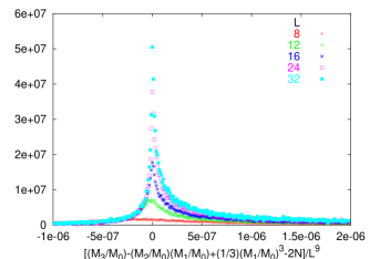
Figure 4: (color online). Distributions, scaled with a factor $L$, for the third term in the specific heat. Each includes $10^{5}$ disorder realizations.

We have also checked distributions for second excitations. The most likely value of $\frac{M_{2}}{M_{0}}-N$ scales as $L^{6}$. We have subtracted off here the (infinite) total number of spins $N$. Single spin flips can occur anywhere and it is sensible to measure the internal energy relative to the unfrustrated system. However, the appropriate contribution to the internal energy is $\frac{M_{2}}{M_{0}}-\frac{1}{2}(\frac{M_{1}}{M_{0}})^{2}-N$. As shown in Fig. 3, the most likely value is close to zero. We note that the mode of $\frac{1}{2}(\frac{M_{1}}{M_{0}}\frac{1}{L^{3}})^{2}$ is roughly $0.002$; indicating a close cancellation. Note also that the shapes of the distributions show clearly the dominant effect of the first excitations. The distributions for third excitations, that is of $\frac{M_{3}}{M_{0}}-\frac{M_{2}}{M_{0}}\frac{M_{1}}{M_{0}}+\frac{1}{3}(\frac{M_{1}}{M_{0}})^{3}-2N$, also show a most likely value close to zero as shown in Fig. 4. Here, the mode of $\frac{M_{3}}{M_{0}}-2N$ scales as $L^{9}$ and the unfrustrated system has $M_{3}=2N$. It is unlikely that higher excitations will interfer with our arguments based on first excitations.

In conclusion, we have reported exact results for the excitations of the bimodal two-dimensional Ising spin glass by expanding in arbitrary temperature from the ground state. All other treatments, except Ref. SK93 , have required extrapolation from definite finite temperatures. We have argued that an energy gap of $2J$ is consistent with $\xi\sim\exp(2J/kT)$ as found from Monte Carlo simulations. The manner in which our model is arranged excludes the possibility of any $2J$ excitation for a finite system. Nevertheless, it should also be interesting to study systems with obvious $2J$ excitations, for example the hexagonal lattice or square lattice with open boundaries or diluted bonds, and investigate the distributions.

W. A. thanks the Commission on Higher Education Staff Development Project, Thailand for a scholarship. J. P. acknowledges fruitful conversations with J. A. Blackman. Some of the computations were performed on the Tera Cluster at the Thai National Grid Center.

References

- (1) A. K. Hartmann and A. P. Young, Phys. Rev. B 64, 180404(R) (2001).
- (2) J. Houdayer, Eur. Phys. J. B 22, 479 (2001).
- (3) J.-S. Wang and R. H. Swendsen, Phys. Rev. B 38, 4840 (1988).
- (4) J. Lukic, A. Galluccio, E. Marinari, O. C. Martin, and G. Rinaldi, Phys. Rev. Lett. 92, 117202 (2004).
- (5) J.-S. Wang, Phys. Rev. E 72, 036706 (2005).
- (6) H. G. Katzgraber, L. W. Lee, and I. A. Campbell, cond-mat/0510668 (2005).
- (7) L. Saul and M. Kardar, Phys. Rev. E 48, R3221 (1993); Nucl. Phys. B 432, 641 (1994).
- (8) T. Jörg, J. Lukic, E. Marinari, and O. C. Martin, Phys. Rev. Lett. 96, 237205 (2006).
- (9) R. Fisch, J. Stat. Phys. 128, 1113 (2007).
- (10) H. G. Katzgraber and L. W. Lee, Phys. Rev. B 71, 134404 (2005).
- (11) R. Sungthong and J. Poulter, J. Phys. A 36, 6347 (2003).
- (12) H. G. Katzgraber, L. W. Lee, and I. A. Campbell, Phys. Rev. B 75, 014412 (2007).
- (13) H. S. Green and C. A. Hurst, Order-Disorder Phenomena (Interscience, London, 1964).
- (14) J. A. Blackman, Phys. Rev. B 26, 4987 (1982).
- (15) J. A. Blackman and J. Poulter, Phys. Rev. B 44, 4374 (1991).
- (16) J. Poulter and J. A. Blackman, Phys. Rev. B 72, 104422 (2005).
- (17) It is convenient to use the bond basis where and are as shown in Fig. 4. of BP91 .
- (18) J. Villain, J. Phys. C 10, 1717 (1977).
- (19) G. André, R. Bidaux, J.-P. Carton, R. Conte, and L. de Seze, J. Phys. (Paris), 40, 479 (1979).
- (20) J. Lukic, E. Marinari, and O. C. Martin, Europhys. Lett. 73, 779 (2006).
- (21) S. Wiseman and E. Domany, Phys. Rev. Lett. 81, 22 (1998).