Interaction of the single-particle and collective degrees of freedom in non-magic nuclei: the role of phonon tadpole terms

Abstract

A method of a consistent consideration of the phonon contributions to mass and gap operators in non-magic nuclei is developed in the so-called $g^{2}$ approximation, where $g$ is the low-lying phonon creation amplitude. It includes simultaneous accounting for both the usual non-local terms and the phonon tadpole ones. The relations which allow the tadpoles to be calculated without any new parameters are derived. As an application of the results, the role of the phonon tadpoles in the single-particle strength distribution and in the single-particle energies and gap values has been considered. Relation to the problem of the surface nature of pairing is discussed.

I introduction

In the last two decades, the progress was achieved in the many-body nuclear theory AB ; Schuck in going beyond the standard RPA or the Theory of Finite Fermi Systems (TFFS) by means of accounting for coupling of the single-particle degrees of freedom with the low-lying collective excitations (“phonons”). For magic nuclei Refs. KhS ; bbb1983 ; ETFFS2004 ; litvaring could be cited, and for nuclei with pairing these are Refs. baranco1999 ; avekaevlet1999 ; milan2 ; avekaev1999 ; tselyaev2007 . For the first studies in this field the use of the phenomenological Saxon-Woods mean field is typical. In this case, a double set of the phenomenological parameters is necessary, the first one for the effective force and the second one for the mean field. Note that in Ref. KhS the main terms of the mean field potential well, i.e. the ones without the phonon corrections, were found in a self-consistent way, within the self-consistent version of the TFFS. However, the phonon characteristics were calculated with the use of the Saxon-Woods potential, thereby the double set of the parameters was used, too.

The characteristic feature of the modern developments in this field is the complete refusal from the phenomenological mean field when both the field and the phonon characteristics are calculated self-consistently, with the use of only one set of parameters for the forces to calculate the mean field. The HFB calculations with the Skyrme forces sarchi ; ave2007 should be cited here and the ones, for magic nuclei only, within the relativistic mean field theory litvaring ; litvaringvret2007 . Article litvaring is an expressive example. Here, in the framework of the old dynamic scheme of ringwerner1973 , the Saxon-Woods mean field was changed by the relativistic mean field. In both studies the authors solved the Dyson equation for the mass operator in the so-called g² approximation, g being the phonon-particle coupling amplitude. Properties of the odd nuclei nearby ²⁰⁸Pb were considered, including the single-particle strength distribution and characteristics of the single-particle levels.

A consistent generalization of the g² approximation to the nuclei with pairing has been performed in avekaev1999 . There Eliashberg’s approach eliashberg1961 , which was developed originally for superconductivity in the solid state physics, has been used and the realistic calculations have been performed for ¹²¹Sn and ¹²³Sn nuclei. In Refs. avekaev1999 ; avekaevlet1999 the problem of evaluating the phonon contribution to the single-particle energies and gap values was consistently formulated and the equations obtained were solved.

The problem of the phonon contribution to the nuclear gap value is, probably, one of the most interesting at present because it is in a close relation to the problem of nature of the nuclear superfluidity. Note that it is also of great interest for the astrophysics, see, e.g., Refs. milan1 ; Baldo05 . As to atomic nuclei themselves, the old problem exists whether the nuclear superfluidity has a volume or surface nature. In the latter case, a question remains in what extent it appears due to a special form of the initial pairing force or to an additional contribution induced by exchange with the collective low-energy surface phonons. The calculations in avekaevlet1999 have shown that we deal with an intermediate case: the phonon contribution to the gap value $\Delta$ for the tin region is about 30% of the experimental gap value, the rest of about 70% being due to the “main” pairing force.

Simultaneously and independently, the problem of nuclear pairing was attacked by the Milan group. They combined an ab initio calculation of the gap starting with the Argonne v₁₄ NN-force, Refs. milan0 ; milan2 , with evaluating the phonon contribution to $\Delta$, Refs. baranco1999 ; milan2 . Their conclusion was that about 50% of the gap value for the tin region appears due to the initial NN-force and the other 50% due to the phonon contribution. Note that the alternative ab initio calculation of the gap was carried out recently in Refs. Pankratov1 (Paris NN-force) and Pankratov2 (Argonne v₁₈ NN-force) on the basis of the method developed in zverevsap2004 . Omitting the discussion of the two methods of solving the ab initio gap equation, note only that a close agreement with the experimental value of $\Delta$ was obtained in Refs. Pankratov1 , Pankratov2 , leaving a room of not more than 20%for the phonon corrections. It agrees qualitatively with the results avekaev1999 ; avekaevlet1999 , but significantly contradicts those of Refs. baranco1999 ; milan2 . It is worth mentioning that in the cited papers by the Milan group the phonon contribution to the gap of Ca and Ti isotopes reaches almost 100%. Thus, a conflicting situation remains in the problem under discussion and new investigations are required to clear up the situation.

However, in all of the above-mentioned papers, and in many other studies dealing with evaluation of the low-lying phonon contribution to nuclear characteristics, a term was lost, which is of the same $g^{2}$ order as the usual non-local pole term of the mass operator taken into account. We mean the so-called tadpole term. It was evaluated firstly in the pioneering paper by V.A. Khodel khod1 and named as the local term. Now we name it, in accordance with the particle physics terminology, as the tadpole diagram. This approach is closely related to the interpretation of the low-lying surface phonons as members of the Goldstone branch which appear due to spontaneous breaking of the translation invariance in nuclei. The ghost $1^{-}$-state with the frequency $\omega_{1}=0$ is the head of this branch, being the exact solution of the self-consistency equation of the TFFS. Therefore, for the simplest version of the TFFS effective force, the corresponding eigenfunction is $g_{1}=\frac{dU}{dr}$, where $U(r)$ is the mean field potential. The TFFS equations for the natural parity excitations will yield small excitation energies $\omega_{L}$ and eigenfunctions $g_{L}$ close to $g_{1}$, provided the self-consistency relation is fulfilled. The main idea of Ref. khod1 was to develop such a scheme of evaluating the surface phonon corrections to nuclear characteristics that they should vanish for the ghost phonon. As it turned out, that is impossible without taking into account the tadpole term.

For magic nuclei the tadpole term was considered in detail in Ref. KhS , see also references therein. As it turned out, the tadpole contribution to the single-particle energies, splitting of the particle-vibration multiplets and other properties of magic nuclei and their odd neighbors are, as a rule, important and are often of the opposite sign as compared with the the usual non-local terms. Development of an analogous approach for non-magic nuclei is a problem of great interest.

The present paper is the first step in this direction. In Section II we derive a closed set of equations for the tadpole operators in nuclei with pairing, which doesn’t contain any new parameters in addition to those used for calculating the mean-field mass operators. In Section III we consider possible approximations to make this set more handy. Closed and transparent relations for the particle-hole (ph) and particle-particle (pp) tadpole terms are obtained. As an application, modifications of the results of Refs. avekaev1999 ; avekaevlet1999 for the single-particle strength distribution and single-particle energies and gap values of superfluid nuclei due to inclusion of the tadpoles are carried out. The relevance of the tadpole terms to the problem of the nature of nuclear pairing is discussed.

II Phonon corrections to the mass and gap operators

In this paper, we deal with the nuclei with weak phonon-particle coupling when the phonon admixture to the one-particle degrees of freedom could be accounted for within a perturbation theory scheme. More specifically, the quantity

$$\alpha=\frac{\bar{g}_{L}^{2}}{(2j+1)\omega_{L}^{2}}$$ (1)

plays the role of the perturbation parameter, and it should be small. Here $\bar{g}_{L}$ is the average value of the matrix element of the $L$-phonon creation amplitude at the Fermi surface, $\omega_{L}$ is its excitation energy, and $j$ is a typical value of the single-particle angular momentum ($j\propto A^{1/3}$). In other words, the coupling strength should be not too high and the excitation energy not too low. We call this as the $g^{2}$ approximation for mass operators.

Such a situation takes place in magic and semi-magic nuclei. There is no pairing at all in the first case and partially, in the magic subsystem, in the second one. For the magic nuclei, the problem under consideration was consistently solved in KhS , see also references therein. Our aim is to develop a similar approach for semi-magic nuclei, with pairing in the non-magic subsystem taken into account.

In the general case of nuclei with pairing it is necessary to consider four one-particle generalized Green functions, i.e. two Green functions, $G$ and $G^{h}$, and two Gor’kov functions $F^{(1)}$ and $F^{(2)}$. In addition to two normal mass operators, $\Sigma$ and $\Sigma^{h}$, their two anomalous counterparts appear. In the textbook Landau they are denoted as $\Sigma_{02}$ and $\Sigma_{20}$, in Refs. avekaevlet1999 ; avekaev1999 as $\Sigma^{(1)}$ and $\Sigma^{(2)}$. Here we use the notation AB , where they are denoted as $\Delta^{(1)}$ and $\Delta^{(2)}$. Therefore we will often name them as the gap operators. Sometimes we use the term ”mass operators“ for all the four quantities under discussion.

The main part of the mass operators is determined by the mean field contribution. In the $g^{2}$ approximation, for the single-particle energy ${\varepsilon}_{\lambda}$ and the average gap value ${\Delta}_{\lambda}$ we have:

$${\varepsilon}_{\lambda}=\Sigma_{\lambda\lambda}={\varepsilon}^{(0)}_{\lambda}+\delta^{(2)}\Sigma_{\lambda\lambda}(\varepsilon_{\lambda}),\hskip 28.45274pt\Delta_{\lambda}=\Delta_{\lambda\lambda}=\Delta_{\lambda\lambda}^{(0)}+\delta^{(2)}\Delta_{\lambda\lambda}(\varepsilon_{\lambda}),$$ (2)

with the obvious notation. In general, the main, mean field, parts of $\Sigma$ and $\Delta$, in the approach discussed, are supposed to be calculated within a self-consistent method, say, the HFB one or the self-consistent TFFS. However, in practice the phenomenological Woods-Saxon potential and pairing force are often used. It should be emphasized that in the latter case it is necessary to use the so-called “refinement” procedure avekaev1999 ; ETFFS2004 in order to avoid a double counting of phonon contribution into the terms ${\varepsilon}^{(0)}_{\lambda}$ and the gap ${\Delta}^{(0)}_{\lambda}$ and to extract the “refined” values from the phenomenological ones. In principle, analogous precautions should be made in the case of the self-consistent calculation with the use of phenomenological forces, too. Indeed, the force parameters should be chosen in such a way that the total expressions (2) (not the ”zero“ ones) would reproduce the experimental values. Note that this very idea was utilized in KhS .

With the use of the $g^{2}$ approximation one can write down the phonon corrections, e.g., to the operators $\Sigma$ and $\Delta^{(1)}$, see Fig.1 and Fig.2, as follows:

+             +             +             +      

Figure 1: Phonon $g^{2}$ corrections to the mass operator $\Sigma(\varepsilon)$ in non-magic nuclei (general case).

+             +             +             +      

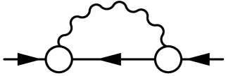
Figure 2: Phonon $g^{2}$ corrections to the gap operator $\Delta^{(1)}(\varepsilon)$ in non-magic nuclei (general case).

$$\delta^{(2)}\Sigma(\varepsilon)={M}(\varepsilon)+K^{ph}\,,$$ (3)

$$\delta^{(2)}\Delta^{(1)}(\varepsilon)={M}^{(1)}(\varepsilon)+K^{pp}\,.$$ (4)

The set of diagrams and the relation for $\delta^{(2)}\Delta^{(2)}$ are absolutely similar to Fig.2 and Eq. (4). In Fig. 1 and Fig. 2 the empty circles denote the phonon creation amplitudes (vertexes). To distinguish between the $g$- and $d$-vertexes it is necessary just to look at the direction of ingoing and outgoing arrows. In the case of one ingoing and one outgoing arrow we deal with the $g$- (or $g^{h}$-) vertex. If there are two ingoing arrows, we deal with the $d^{(1)}$-vertex, two outgoing arrows mean the $d^{(2)}$-vertex. The terms with two phonon creation amplitudes are the energy dependent non-local operators, the sums of them being denoted as $M$ and $M^{(1)}$. The last terms are the corresponding ph- and pp-phonon tadpoles. The essential property of these tadpoles is that they do not depend on the energy $\varepsilon$.

The explicit expressions for the phonon tadpoles K^ph and K ^pp are given by

$$K^{ph}=\int\frac{d\omega}{2\pi i}D(\omega)\delta g(\omega)\,,$$ (5)

$$K^{pp}=\int\frac{d\omega}{2\pi i}D(\omega)\delta d^{(1)}(\omega)\,,$$ (6)

where D is the phonon Green function and $\delta g$ and $\delta d^{(1)}$ are the changes of the ph- and pp-phonon creation amplitudes in the external field of another phonon with the same quantum numbers as the one whose contribution we analyze.

II.1 Magic nuclei

To begin with, let us first outline briefly the method for magic nuclei, following to KhS . In this case there is no pairing and only the first and the last terms in Fig. 1 for the corrections to the mass operator $\Sigma$ survive. The first term is the usual pole diagram, where the Green function G, of course, does not contain pairing effects. The last term means the sum of all the irreducible diagrams. In the problem under consideration, as it was mentioned in the Introduction, this sum was evaluated firstly in Ref. khod1 . We name it, in accordance with the particle physics terminology, as the tadpole diagram.

The second order in $g_{L}$ correction to the mass operator $\Sigma$ reads

$$\delta_{LL}^{(2)}\Sigma(\varepsilon)=\int\frac{d\omega}{2\pi i}S_{LL}(\varepsilon,\omega)D_{L}(\omega),$$ (7)

where $D_{L}$ stands for the $L$-phonon $D$-function and $S_{LL}$ is the phonon-particle scattering amplitude. As usual, the symbolic multiplication means the integration over intermediate coordinates and summation over the spin variables. In accordance with Fig.1, $S_{LL}$ is the sum

$$S_{LL}=g_{L}Gg_{L}+\delta_{L}{g_{L}}\,,$$ (8)

where $\delta_{L}{g_{L}}$ is the tadpole term. Obviously, it is of the second order correction to $\Sigma$, as far as the first order correction to $\Sigma$ is the particle-phonon interaction amplitude, $g_{L}=\delta_{L}\Sigma$. According to the recipe of KhS , it can be found by the direct variation of the equation for the vertex $g_{L}$,

$$g_{L}={\cal F}Ag_{L},$$ (9)

where ${\cal F}$ is the Landau–Migdal effective NN-interaction amplitude AB and $A=GG$ is the particle-hole propagator. After the variation of Eq.(9) over the phonon creation amplitude one obtains:

$$\delta_{L}g_{L}=({\delta_{L}\cal F})Ag_{L}+{\cal F}(\delta_{L}A)g_{L}+{\cal F}A\;\delta_{L}g_{L}.$$ (10)

This is an integral equation for the quantity $\delta_{L}g_{L}$ with the inhomogeneous term

$$m_{LL}=(\delta_{L}{\cal F})Ag_{L}+{\cal F}(\delta_{L}A)g_{L}.$$ (11)

The procedure of finding the second term of the inhomogeneous term is quite obvious. The direct variation of the particle-hole propagator yields:

$$(\delta_{L}A)=2G(\delta_{L}G)=2GGg_{L}G.$$ (12)

Up to now, we have used a symbolic notation. To obtain the explicit relations, let us, for simplicity, suppose that the mass operator $\Sigma$ is momentum independent. In this case, we have for the first order correction

$$\delta_{LM}^{(1)}\Sigma({\bf r})=g_{LM}({\bf r})=g_{L}(r)Y_{LM}({\bf n}).$$ (13)

Note that within the Bohr–Mottelson (BM) liquid drop model one has

$$g_{L}^{\rm BM}(r)=\alpha_{L}\frac{dU(r)}{dr},$$ (14)

where $U(r)$ stands for the nuclear mean field potential and $\alpha_{L}$ is the constant which determines the amplitude of the surface vibration. As it was demonstrated in KhS , the direct solution of the RPA-like equation (9) for a low-lying excitation in an even-even nucleus is very close to the BM model prescription (14). Therefore, for qualitative estimations, one can use this simplified form of the particle-phonon vertex.

To obtain the second term in (11) we could fold the quantity (12) with $g_{L}$. Let us introduce the notation $T=\delta_{L}Ag_{L}$. In the explicit form, with the help of (12), we obtain

$$T_{LM_{1}LM_{2}}({\bf r},\omega) = \int\frac{d\varepsilon}{2\pi i}d{\bf r}_{1}d{\bf r}_{2}G({\bf r},{\bf r}_{1};\varepsilon)g_{LM_{1}}({\bf r}_{1})$$ (15)

$$\times \left[G({\bf r}_{1},{\bf r}_{2};\varepsilon-\omega)+G({\bf r}_{1},{\bf r}_{2};\varepsilon+\omega)\right]g_{LM_{2}}({\bf r}_{2})G({\bf r}_{2},{\bf r};\varepsilon).$$

The problem of finding the first term of (11) looks less obvious. To find it, an ansatz was used in KhS based on the density dependence of the Landau–Migdal amplitude $\cal{F}$,

$$\delta_{L}{\cal F}=\frac{\delta{\cal F}}{\delta\rho}\delta_{L}\rho,$$ (16)

where $\delta_{L}\rho$ is the transition density associated with the $L$-phonon excitation. It obeys the relation

$${\delta_{L}\rho}=Ag_{L}.$$ (17)

In the approximation similar to (14), we have

$$({\delta_{L}\rho})^{\rm BM}(r)=\alpha_{L}\frac{d\rho(r)}{dr}.$$ (18)

Thus, the equation for the ph-tadpole in magic nuclei reads

$$K^{ph}=\delta_{L}{\cal F}AgD+{\cal F}(\delta_{L}A)g_{L}D+{\cal F}AK^{ph}.$$ (19)

In the graphic form this equation is shown in Fig. 3.

= + +

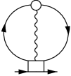
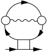
Figure 3: Equation for the tadpole in magic nuclei

II.2 Non-magic nuclei

As it was discussed above, in the general case of nuclei with pairing, in addition to the one-particle Green function $G$, two Gor’kov functions $F^{(1,2)}$ enter the TFFS relations, and two gap functions $\Delta^{(1,2)}$ appear in addition to the mass operator $\Sigma$. They are related to each others,

$$\Delta^{(1,2)}={\cal F}^{\xi}F^{(1,2)},$$ (20)

in terms of the interaction amplitude ${\cal F}^{\xi}$ irreducible in the particle-particle channel. It should be noted that hereafter we mean that the Green function $G$ takes the superfluidity effects into account.

In the systems with pairing, Eq.(9) for the phonon-particle vertex is generalized and two new amplitudes appear AB :

$$d^{(1,2)}_{LM}({\bf r})=\delta_{LM}\Delta^{(1,2)}({\bf r})=d^{(1,2)}_{L}(r)Y_{LM}({\bf n}).$$ (21)

Let us omit for a while the subscripts and upper indices. As far as the amplitude ${\cal F}^{\xi}$ in the TFFS is considered to be density dependent SapTr ; ZverSap ; Fay , two terms in (21) appear:

$$d={\cal F}^{\xi}\delta F+\delta{\cal F}^{\xi}F.$$ (22)

It is worth pointing out that usually the first term in (22) is only taken into account. V.A. Khodel khod2 was, evidently, the first who turned attention to the second one. It is natural to use for it the ansatz analogous to (16):

$$\delta_{L}{\cal F}^{\xi}=\frac{\delta{\cal F}^{\xi}}{\delta\rho}\delta_{L}\rho,$$ (23)

but now, due to pairing effects, the transition density obeys the equation which is more complicated than Eq. (17). It will be written down below.

To introduce the standard TFFS notation, let us omit for a while the second term in Eq. (22). As far as we deal with the low-lying excitations of natural parity, contributions of spin-dependent forces could be neglected in the equations for g and g^h AB . As the result, the relation $g^{h}=g$ is valid. In this case, the quantities $g_{L}$ and $d^{(1,2)}$ obey the set of equations AB , which could be written in the form similar to (9),

$${\hat{g}}={\hat{\cal F}}{\hat{A}}{\hat{g}},$$ (24)

but now all the ingredients of (24) are matrices:

$${\hat{g}}=\left(\begin{array}[]{c}g\\ d^{(1)}\\ d^{(2)}\end{array}\right)\,,$$ (25)

$${\hat{\cal F}}=\left(\begin{array}[]{ccc}{\cal F}&0&0\\ 0&{\cal F}^{\xi}&0\\ 0&0&{\cal F}^{\xi}\end{array}\right),$$ (26)

$${\hat{A}}=\left(\begin{array}[]{ccc}{\cal L}&{\cal M}^{(1)}&{\cal M}^{(2)}\\ {\cal O}&{\cal N}^{(1)}&{\cal N}^{(2)}\\ \tilde{\cal O}&\tilde{\cal N}^{(1)}&\tilde{\cal N}^{(2)}\end{array}\right)\,.$$ (27)

Here ${\cal L},\;{\cal M}^{(1)}$, and so on, denote integrals over $\varepsilon$ of different double products of the Green function $G(\varepsilon)$ and Gor’kov functions, $F^{(1)}(\varepsilon)$ and $F^{(2)}(\varepsilon)$. They could be found in AB and we write down now explicitly only two of them,

$${\cal L}(\omega)=\int\frac{d\varepsilon}{2\pi i}\left[G(\varepsilon)G(\varepsilon+\omega)-F^{(1)}(\varepsilon)F^{(2)}(\varepsilon+\omega)\right],$$ (28)

and

$${\cal O}(\omega)=-\int\frac{d\varepsilon}{2\pi i}\left[G(\varepsilon)F(\varepsilon+\omega)+F(\varepsilon)G(-\varepsilon-\omega)\right].$$ (29)

Let us come back to the second term of (23). With the help of the above short notation the transition density could be written in a compact form similar to (17):

$${\delta\rho}=\sum_{i}A_{1i}g_{i}.$$ (30)

Using this relation, we may express the term under consideration in terms of the “generalized vertex function” $\hat{g}$:

$$\delta{\cal F}^{\xi}=\frac{\delta{\cal F}^{\xi}}{\delta\rho}\sum_{i}A_{1i}g_{i}.$$ (31)

By substituting this relation to (23) we find that the general structure of Eq. (24) remains valid, but now the “interaction matrix” $\hat{\cal F}$ becomes more complicated, in particular, non-diagonal. To be more exact, the first line of (26) remains unchanged, but new non-diagonal terms appear in two other lines. To simplify their explicit form, let us use the approximation for the effective pairing interaction amplitude ${\cal F}^{\xi}$ which is usually utilized in the TFFS (e.g., see Fay ). Namely, it is considered as an energy independent delta-force with a density dependent strength ${\cal F}^{\xi}(\rho({\bf r}))$. In this case, the second term of (22) is reduced to

$$\delta{\cal F}^{\xi}F=\frac{d{\cal F}^{\xi}}{d\rho}\;{\delta\rho}({\bf r})\;\chi({\bf r}),$$ (32)

where

$$\chi({\bf r})=\int\frac{d\varepsilon}{2\pi i}F(\varepsilon,{\bf r},{\bf r})$$ (33)

is the anomalous density. Combining the above relations, one can readily find two new non-diagonal terms of the matrix $\hat{\cal F}$,

$${\cal F}_{21}={\cal F}_{31}=\frac{d{\cal F}^{\xi}}{d\rho}\;\chi({\bf r}).$$ (34)

Thus, we obtain the matrix equation (24) for $\hat{g}$ in the general case where both terms of Eq. (22) are taken into account. After variation of this equation over the field of the surface $L$-phonon under consideration we find the matrix equation for the tadpole term in a superfluid nucleus:

$$\delta_{L}\hat{g}_{L}=(\delta_{L}\hat{\cal F})\hat{A}\hat{g}_{L}+\hat{\cal F}(\delta_{L}\hat{A})\hat{g}_{L}+\hat{\cal F}\hat{A}\;\delta_{L}\hat{g}_{L}.$$ (35)

In principle, this set of equations solves the problem of finding the tadpole terms under discussion. In accordance with Eqs. (3),(4), they should be obtained by folding the solutions of Eq. (35) with the phonon $D$-function. However, the explicit form of this equation is quite cumbersome. The second term on the r.h.s. of Eq. (35) is the most complicated. To find $\delta{\cal L}$ and variations of other components of the $\hat{A}$ matrix, one can use the well known expressions for $\delta G$, $\delta G^{h}$, $\delta F^{(1,2)}$ AB . In the result, one obtains a lot of integrals of triple combinations of the Green and Gor’kov functions of the type of Eq. (15). To obtain more handy relations, some approximations should be made.

III Small $d$ approximation

As it was discussed in the Introduction, the collectivity of the low-lying ph-phonons, i.e. the surface vibrations, exceeds significantly that of the pp-phonons, i.e. the pairing vibrations. Therefore, we concentrate here on the contributions to the mass and gap operators of the phonons of the first type. In this case, the $g_{L}$ component of the generalized vertex $\hat{g}_{L}$ dominates in Eqs. (24) and (35) and the inequality $g\gg d^{(1,2)}$ is valid. For this reason, we can omit the terms with the pairing phonon creation amplitudes $d^{(1,2)}$ in these equations and, correspondingly, in Figs. 1,2. In this approximation, the diagrams depicted in Figs. 4,5 should only be taken into account . In addition, we assume that we deal with the “developed pairing” case when pairing properties of neighboring even-even nuclei should be considered identical. In this case, we have $\Delta^{(1)}=\Delta^{(2)}=\Delta$ and $d^{(1)}(\omega)=\pm d^{(2)}(-\omega)=d(\omega)$AB . The sign “+” takes place for the states of natural parity we consider. The appropriate explicit expressions for $M(\varepsilon)$=$M^{h}(-\varepsilon)$ and $M^{(1)}(\varepsilon)$=$M^{(2)}(\varepsilon)$ are given in avekaev1999 .

+      

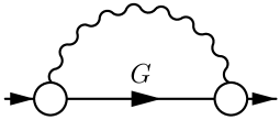
Figure 4: Phonon $g^{2}$corrections to the mass operator $\Sigma(\varepsilon)$ in non-magic nuclei in the small $d$ approximation (the Green function G contains pairing effects).

+      

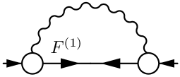
Figure 5: Phonon $g^{2}$corrections to the gap operator $\Delta^{(1)}(\varepsilon)$ in non-magic nuclei in the small $d$ approximation.

In the approximation under consideration, instead of the set (24), we obtain the closed equation for $g$,

$$g={\cal F}{\cal L}g\,,$$ (36)

and the closed expression for the $d$-vertex in terms of $g$:

$$d(\omega)=\left({\cal F}_{21}{\cal L}(\omega)+{\cal F}^{\xi}{\cal O}(\omega)\right)g.$$ (37)

Sometimes the initial equation (22) for the $d$-vertex is more convenient. In the small $d$ approximation, it reads:

$$d(\omega)={\cal F}^{\xi}{\cal O}(\omega)g+\delta{\cal F}^{\xi}F\,.$$ (38)

The set of Eqs. (35) for the tadpole terms is also simplified. It could be obtained either by omitting terms containing $d^{(1)},d^{(2)}$ in (35) or by the direct variation of Eqs. (36) and (37). In the result, one receives:

$$\delta g=\delta{\cal F}{\cal L}g+{\cal F}\delta{\cal L}g+{\cal F}{\cal L}\delta g,$$ (39)

$$\delta d=\delta{\cal F}_{21}{\cal L}g+{\cal F}_{21}\delta{\cal L}g+\delta{\cal F}^{\xi}{\cal O}g+{\cal F}^{\xi}\delta{\cal O}g+\left({\cal F}_{21}{\cal L}+{\cal F}^{\xi}{\cal O}\right)\delta g\,.$$ (40)

Thus, we obtained the integral equation (39) for $\delta g$ with the inhomogeneous term, which is similar to the $m_{LL}$ term (11) for magic nuclei, and expression (40) for $\delta d$. The latter contains $\delta g$ and four terms, which are analogous to the inhomogeneous terms of the equation for the $\delta g$. Let us consider them in detail.

An alternative relation for $\delta d$ could be found by variation of Eq. (38). It is as follows:

$$\delta d=\delta{\cal F}^{\xi}{\cal O}g+{\cal F}^{\xi}\delta{\cal O}g+\delta{\cal F}^{\xi}\delta F+(\delta^{2}{\cal F}^{\xi})F+{\cal F}^{\xi}{\cal O}\delta g\,.$$ (41)

To obtain the quantities $\delta{\cal L}$ and $\delta{\cal O}$ in the equations discussed above in the explicit form, one should variate the propagators ${\cal L}$ and ${\cal O}$:

$$\delta{\cal L}=\delta(GG-F^{(1)}F^{(2)})\,,$$ (42)

$$\delta{\cal O}=\delta(GF^{(1)}+F^{(1)}G^{h}),$$ (43)

and use the small $d$ approximation, omitting the terms with $d^{(1)},d^{(2)}$ in the general expressions for the variation of the Green functions AB . One obtains:

$$\delta G=GgG-F^{(1)}gF^{(2)},\hskip 28.45274pt\delta G^{h}=G^{h}gG^{h}-F^{(2)}gF^{(1)}\,,$$ (44)

$$\delta F^{(1)}=GgF^{(1)}+F^{(1)}g^{h}G^{h},\hskip 28.45274pt\delta F^{(2)}=F^{(2)}gG+G^{h}g^{h}F^{(2)}\,.$$ (45)

For a time, we come back to the notation $F^{(1)},F^{(2)},G^{h}$ to avoid an explicit specification of the energy variables in the integrals similar to that in Eq. (15), which appear after folding expressions (42) and (43) with $g$. They could be obtained by combining Eqs.(42)-(45) and, in the symbolic form, are as follows:

$$\delta{\cal L}g= g(GGG-F^{(1)}F^{(2)}G+GGG-GF^{(1)}F^{(2)}-$$ (46)

$$GF^{(1)}F^{(2)}-F^{(1)}GF^{(2)}-F^{(1)}F^{(2)}G-F^{(1)}G^{h}F^{(2)})g\,,$$

and

$$-\delta{\cal O}g=g(GGF^{(1)}-F^{(1)}F^{(2)}F^{(1)}+GGF^{(1)}+GF^{(1)}G^{h}+$$

$$GF^{(1)}G^{h}+F^{(1)}G^{h}G^{h}+F^{(1)}G^{h}G^{h}-F^{(1)}F^{(2)}F^{(1)})g\,.$$ (47)

Thus, even for the simplified case under consideration, we obtained eight terms for $\delta{\cal L}g$ instead of the one in Eq. (10). In addition to them, eight new terms for $\delta{\cal O}g$ appear in the expression for $\delta d$. The explicit form of each integral entering Eqs. (46),(47) is similar to that of Eq. (15).

III.1 Final relationships for the tadpoles

For magic nuclei, equation (19) for the tadpole term was solved in the coordinate representation KhS . Even in this case the procedure turned out to be quite cumbersome. In principle, this method could be generalized to the systems with pairing, using the coordinate representation for the Green and Gor’kov functions fayansbelyaev . However, as it is clear from the above formulas, in this case it will be much more complicated. For this reason, we prefer to use the representation of the single-particle wave functions, the so-called $\lambda$-representation. To make the final equations for the tadpoles more transparent, we also use the diagonal in $\lambda$ approximation. The matter is that the set $\{\lambda\}$ is chosen in such a way that the mean field mass operator $\Sigma^{(0)}$ and the corresponding Green function $G^{(0)}$ are diagonal in $\lambda$. We use the approximation supposing that the mean field gap function $\Delta^{(0)}$, the Green function $G$ with pairing and Gor’kov functions $F^{(1,2)}$ are also diagonal in $\lambda$ AB . In this approximation, ${\cal L},{\cal O}$ and other two-particle propagators contain two $\lambda$-subscripts, ${\cal L}_{\lambda_{1}\lambda_{2}}$ and so on, whereas in the general case we have ${\cal L}_{\lambda_{1}\lambda_{2}}\to{\cal L}_{\lambda_{1}\lambda_{2}\lambda_{3}\lambda_{4}}$, etc. The corresponding generalization of the equations written down below is quite obvious.

The equations for the tadpoles are obtained by substitution of Eqs. (39) and (40) (or (41)) into Eqs. (5) and (6). The final equation for the K^ph tadpole, in the obvious short notation, has the form:

$$K^{ph}_{12}=\sum_{3,4}\int\frac{d\varepsilon}{2\pi i}\frac{d\omega}{2\pi i}\;\delta{\cal{F}}_{1234}(\omega){\cal L}_{34}(\varepsilon,\omega)g_{34}D_{L}(\omega)+$$

$$\sum_{3,4}{\cal{F}}_{1234}\int\frac{d\varepsilon}{2\pi i}\frac{d\omega}{2\pi i}(\delta{\cal{L}}g)_{34}(\varepsilon,\omega)D_{L}(\omega)+$$

$$\sum_{3,4}{\cal{F}}_{1234}\int\frac{d\varepsilon}{2\pi i}{\cal{L}}_{34}(\varepsilon,\omega_{L})K^{ph}_{34}\,.$$ (48)

For the K^pp tadpole, let us first use Eq. (41) for $\delta d$. We find:

$$K^{pp}_{12}=2\sum_{3,4}\int\frac{d\varepsilon}{2\pi i}\frac{d\omega}{2\pi i}\delta{\cal{F}^{\xi}}_{1234}(\omega){\cal O}_{34}(\varepsilon,\omega)g_{34}D_{L}(\omega)+$$

$$\sum_{3,4}{\cal F}^{\xi}_{1234}\int\frac{d\varepsilon}{2\pi i}\frac{d\omega}{2\pi i}(\delta{\cal{O}}g)_{34}(\varepsilon,\omega)D_{L}(\omega)+$$

$$\sum_{3}\int\frac{d\varepsilon}{2\pi i}\frac{d\omega}{2\pi i}\delta^{(2)}{\cal{F}^{\xi}}_{1233}(\omega)F_{3}(\varepsilon)D_{L}(\omega)+$$

$$\sum_{3,4}{\cal{F}^{\xi}}_{1234}\int\frac{d\varepsilon}{2\pi i}{\cal{O}}_{34}(\varepsilon,\omega_{L})K^{ph}_{34}\,.$$ (49)

The factor 2 in the first term in Eq. (49) appears due to the fact that, in the small $d$ approximation, the terms $\delta{\cal F}^{\xi}{\cal O}g$ and $\delta{\cal F}^{\xi}\delta F^{1}$ in Eq. (41) are equal to each other.

= + +

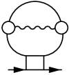
Figure 6: Equation for the tadpole $K^{ph}$ in non-magic nuclei in the small $d$ approximation.

= 2 + + +

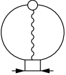
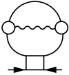
Figure 7: Expression for the tadpole $K^{pp}$ in non-magic nuclei in the small $d$ approximation.

In the graphic form, Eqs. (48) and (49) are illustrated in Fig. 6 and Fig. 7 respectively. For the sake of simplicity, contrary to Fig. 3, here we do not draw all the internal Green functions and omit arrows for those which are drawn. The arrows are only conserved in the cases where it is necessary for understanding. In particular, in the last diagrams of both figures the arrows show that we deal with the tadpole $K^{ph}$. Remember that the second term on the r.h.s. of Eq. (48) in the detailed presentation includes 8 particular diagrams, in accordance with Eq. (46). In the case of $K^{pp}$ tadpole, the number of diagrams is even larger. Therefore the detailed diagram representation of Eqs. (48) and (49) is rather complicated.

Eq. (49) is convenient for the graphical representation, but it possesses one drawback: it contains the term with $\delta^{(2)}{\cal{F}^{\xi}}$ with the “hidden” tadpole $K^{ph}$. To separate the latter one explicitly it is necessary to use Eq. (40) instead of (41). In the result, we find:

$$K^{pp}_{12}=\sum_{3,4}\int\frac{d\varepsilon}{2\pi i}\frac{d\omega}{2\pi i}(\delta_{L}{\cal F}_{21})_{1234}(\omega){\cal L}_{34}(\varepsilon,\omega)g_{34}D_{L}(\omega)+$$

$$\sum_{3,4}\int\frac{d\varepsilon}{2\pi i}\frac{d\omega}{2\pi i}\delta{\cal{F}^{\xi}}_{1234}(\omega){\cal O}_{34}(\varepsilon,\omega)g_{34}D_{L}(\omega)+$$

$$\sum_{3,4}({\cal F}_{12})_{1234}\int\frac{d\varepsilon}{2\pi i}\frac{d\omega}{2\pi i}(\delta{\cal{L}}g)_{34}(\varepsilon,\omega)D_{L}(\omega)+$$

$$\sum_{3,4}{\cal F}^{\xi}_{1234}\int\frac{d\varepsilon}{2\pi i}\frac{d\omega}{2\pi i}(\delta{\cal{O}}g)_{34}(\varepsilon,\omega)D_{L}(\omega)+$$

$$\sum_{3,4}\left[({\cal F}_{21})_{1234}\int\frac{d\varepsilon}{2\pi i}{\cal{L}}_{34}(\varepsilon,\omega_{L})+{\cal{F}^{\xi}}_{1234}\int\frac{d\varepsilon}{2\pi i}{\cal{O}}_{34}(\varepsilon,\omega_{L})\right]K^{ph}_{34}\,.$$ (50)

One remark should be made concerning the integrals over $\omega$ in the above equations for the tadpoles. The poles of the $D$-function should be taken into account only because they lead to the terms which strongly depend on the low-laying phonon frequency $\omega_{L}$ and other phonon characteristics. They could change significantly from one nucleus to another. On the other hand, the terms appearing due to poles of ${\cal L}$, ${\cal O}$ and other two-particle propagators do not practically depend on $\omega_{L}$. They are smooth functions of all the variables under consideration and should be included into the corresponding mean-field quantities.

The solution of the integral equations (48) and (49) (or (50)) yields the tadpole values which, according to Eqs. (2) and (3), should be added to the usual non-local terms. Note that in the approach discussed there is no need for any new parameters. Below we consider some applications of the results obtained.

III.2 Applications to description of the single-particle characteristics of non-magic nuclei

In Refs. avekaev1999 ; avekaevlet1999 the approach to describe the the single-particle strength distribution for non-magic odd nuclei and to take into account the phonon contributions to the single-particle energies and gap values has been developed on the basis of generalization of the Eliashberg theory eliashberg1961 to nuclei, with the first application of the Eliashberg theory to nuclei made in kadmluk1989 . The general set of equations of Refs. avekaev1999 ; avekaevlet1999 for the energy and gap operators, with account for the dynamic spread of a single-particle level (the “dynamic” case), has been derived in the diagonal approximation for the mass and gap operators. (Arguments in favor of such an approximation could be found in avekaev1999 ; avekaevlet1999 ). The equations are as follows :

$$\varepsilon_{\lambda\eta}=\frac{\varepsilon_{\lambda}^{(0)}+M^{\rm even}_{\lambda}(E_{\lambda\eta})}{1+q_{\lambda\eta}(E_{\lambda\eta})}\,,$$

$$\Delta_{\lambda\eta}=\frac{\Delta_{\lambda}^{(0)}+M^{(1)}_{\lambda}(E_{\lambda\eta})}{1+q_{\lambda\eta}(E_{\lambda\eta})}\,,$$

$$E_{\lambda\eta}=\sqrt{\varepsilon_{\lambda\eta}^{2}+\Delta_{\lambda\eta}^{2}}\,,$$ (51)

where

$$q_{\lambda\eta}=-\frac{M^{\rm odd}_{\lambda}(E_{\lambda\eta})}{E_{\lambda\eta}}\,.$$ (52)

Here $M^{\rm even}$ and $M^{\rm odd}$ are even and odd in energy components of the non-local mass operator $M$ ($M=M^{\rm even}+M^{\rm odd}$), which enters the r.h.s. of Eq. (3), and $M^{(1)}$ is the same as in Eq. (4). The subscript $\eta$ numerates solutions of the set of Eqs.(51),(52). This yields the distribution of the single-particle strength in non-magic nuclei.

In order to obtain the single-particle energies and gap values (the “static” case) from Eqs. (51),(52), it is necessary, for each $\lambda$, to separate the dominant solution $\eta$ from the set $\{\lambda\eta\}$. For this aim, the spectroscopic factors should be analyzed. They are given avekaev1999 with

$$S^{\pm}_{\lambda\eta}=\frac{(1+q_{\lambda\eta})(E_{\lambda\eta}\pm\varepsilon_{\lambda\eta})}{\dot{\Theta}_{\lambda}(E_{\lambda\eta})}\,,$$ (53)

where

$$\Theta_{\lambda}(\varepsilon)=(\varepsilon-\varepsilon^{(0)}_{\lambda}-M_{\lambda}(\varepsilon))(\varepsilon+\varepsilon^{(0)}_{\lambda}+M_{\lambda}^{h}(\varepsilon))-(\Delta^{(0)}_{\lambda}+M^{(1)}_{\lambda}(\varepsilon))^{2}.$$ (54)

The $\eta$-component with the maximal spectroscopic factor should be associated with the experimental single-particle level, the details see in avekaev1999 . Let us denote the observed single-particle energies and gap values as $\varepsilon_{\lambda}$ and $\Delta_{\lambda}$ and the corresponding mean field values as $\varepsilon^{(0)}_{\lambda}$ and $\Delta^{(0)}_{\lambda}$. They are related to each other by Eqs. (51),(52) with $\eta$ equal to the dominant value. Let us rewrite them explicitly, omitting the subscript $\eta$:

$$\varepsilon_{\lambda}=\frac{\varepsilon^{(0)}_{\lambda}+M^{\rm even}_{\lambda}(E_{\lambda})}{1+q_{\lambda}(E_{\lambda})}\,,$$

$$\Delta_{\lambda}=\frac{\Delta_{\lambda}^{(0)}+M^{(1)}_{\lambda}(E_{\lambda})}{1+q_{\lambda}(E_{\lambda})}\,,$$

$$E_{\lambda}=\sqrt{\varepsilon_{\lambda}^{2}+\Delta_{\lambda}^{2}}\,,$$ (55)

where

$$q_{\lambda}=-\frac{M^{\rm odd}_{\lambda}(E_{\lambda})}{E_{\lambda}}\,.$$ (56)

The energies $\varepsilon_{\lambda}$ and $\varepsilon_{\lambda}^{(0)}$ are reckoned from the corresponding chemical potentials $\mu$ and $\mu^{(0)}$. Note that in Refs. avekaev1999 ; avekaevlet1999 the phenomenological Saxon-Woods potential was utilized as the mean field one and the phenomenological pairing forces were used as well. As far as both of them are adjusted to the observed values of $\varepsilon_{\lambda}$ and $\Delta_{\lambda}$, a special “refinement” procedure mentioned above is necessary to find $\varepsilon^{(0)}_{\lambda}$ and $\Delta^{(0)}_{\lambda}$ values. It is described in detail in the cited articles.

Now it is necessary to modify these results in order to include the tadpoles in accordance with Eqs. (3), (4). In fact, there was no specialization of the mass operators in avekaev1999 ; avekaevlet1999 to derive the relations (51) and (55). For this reason, in order to include the tadpoles into consideration we should just change the mass and gap operators of Refs. avekaev1999 ; avekaevlet1999 to the ones from Eqs. (3) and (4). Remember that the tadpole terms K^ph and K^pp do not depend on the energy. Supposing, just as the non-local operators $M,M^{(1)}$, that they are diagonal in $\lambda$, we obtain

$$\varepsilon_{\lambda\eta}=\frac{\varepsilon^{(0)}_{\lambda}+M^{\rm even}_{\lambda}(E_{\lambda\eta})}{1+q_{\lambda\eta}(E_{\lambda\eta})}+\frac{K^{ph}_{\lambda}}{1+q_{\lambda\eta}(E_{\lambda\eta})}\,,$$

$$\Delta_{\lambda\eta}=\frac{\Delta^{(0)}_{\lambda}+M^{(1)}_{\lambda}(E_{\lambda\eta})}{1+q_{\lambda\eta}(E_{\lambda\eta})}+\frac{K^{pp}_{\lambda}}{1+q_{\lambda\eta}(E_{\lambda\eta})}\,,$$

$$E_{\lambda\eta}=\sqrt{\varepsilon_{\lambda\eta}^{2}+\Delta_{\lambda\eta}^{2}}\,,$$ (57)

with

$$q_{\lambda\eta}=-\frac{M^{\rm odd}_{\lambda\eta}(E_{\lambda\eta})}{E_{\lambda\eta}}\,,$$ (58)

instead of Eqs. (51),(52). In the same way, instead of Eqs. (55),(56) for the single-particle and gap values, we find:

$$\varepsilon_{\lambda}=\frac{\varepsilon^{(0)}_{\lambda}+M^{\rm even}_{\lambda}(E_{\lambda})}{1+q_{\lambda}(E_{\lambda})}+\frac{K^{ph}_{\lambda}}{1+q_{\lambda}(E_{\lambda})}\,,$$

$$\Delta_{\lambda}=\frac{\Delta^{(0)}_{\lambda}+M^{(1)}_{\lambda}(E_{\lambda})}{1+q_{\lambda}(E_{\lambda})}+\frac{K^{pp}_{\lambda}}{1+q_{\lambda}(E_{\lambda})}\,,$$

$$E_{\lambda}=\sqrt{\varepsilon_{\lambda}^{2}+\Delta_{\lambda}^{2}}\,,$$ (59)

with

$$q_{\lambda}=-\frac{M^{\rm odd}_{\lambda}(E_{\lambda})}{E_{\lambda}}\,.$$ (60)

We see that both the single-particle energy and gap values are changed due to inclusion of the tadpoles, both in the dynamic and static cases. In the latter case, the solution of the set of Eqs. (59) should answer the question about the total phonon contribution, including the tadpole terms, to the pairing gap, as compared with the mean field, or ”refined“, value $\Delta^{(0)}_{\lambda}$. Up to now, all calculations of the phonon corrections to the gap have ignored the tadpole contributions.

Let us briefly discuss the situation in nuclei without pairing. In this case, the equations of Sect. II A for the phonon corrections to the single-particle energies were solved in the coordinate representation in KhS (see references therein, in particular, platonov1980 ). It turned out that the tadpole contribution to $\varepsilon_{\lambda}$ was, as a rule, significant and comparable with that of the non-local term of the mass operator. For a qualitative analysis, we limit ourselves with the diagonal in $\lambda$ approximation, using Eqs. (57) and (59) without any pairing contribution. For the spread of a single-particle state we have:

$$\varepsilon_{\lambda\eta}=\varepsilon^{(0)}_{\lambda}+M_{\lambda}(\varepsilon_{\lambda\eta})+K^{ph}_{\lambda}\,,$$ (61)

and for the single-particle energies:

$$\varepsilon_{\lambda}=\varepsilon^{(0)}_{\lambda}+M_{\lambda}(\varepsilon_{\lambda})+K^{ph}_{\lambda}\,.$$ (62)

As far as K^ph does not depend on the energy, the shift of the solutions, for a fixed $\lambda$, will be the same for all the values of $\eta$. For the same reason, that is independence of K^ph on energy, the spectroscopic factors which are determined by the residues of the Green function and, therefore, by the energy derivative of the mass operator in Eq. (3), are not changed.

This conclusion about the role of the ph-tadpole in magic nuclei agrees with the results of calculations for single-particle level properties in odd neighbors of ²⁰⁸Pb in Ref. litvaring cited above, where the tadpole contribution was not taken into account. Indeed, as it can be seen from Table III of litvaring , the authors obtained a good agreement with the experiments for the spectroscopic factors, where there is no tadpole contribution, but the agreement for the single-particle energies is considerably worse due to the fact that in this case the tadpole contribution does exist.

Things are different in nuclei with pairing. In this case, in the absence of the tadpole, the single-particle spectroscopic factors are given with Eqs. (53),(54). If the tadpole terms $K^{ph}$ and $K^{pp}$ are included, as it can be easily checked, in addition to a change of $E_{\lambda\eta}$ and $\varepsilon_{\lambda\eta}$, the expression (53) itself is modified. Thus, for non-magic nuclei both the energies and spectroscopic factors should be changed due to inclusion of the tadpoles.

IV Conclusion

In this work, a consistent approach is developed to include the phonon coupling in the $g^{2}$ approximation for mass and gap operators in non-magic nuclei with explicit consideration of the tadpole terms, in addition to the usual non-local terms. The general set of equations for the phonon corrections under discussion is obtained, which doesn’t include any new parameters besides those used in the self-consistent calculation of the “zero” mean field, i.e. the ones without phonon contributions. This set is simplified for the case of corrections induced by low-lying surface phonons in the “small $d$ approximation” ($d^{(1,2)}<<g$). This approximation means that the admixture of pp-phonons with ph-phonons under consideration, i.e. the contribution of the $d^{(1,2)}$-vertexes in comparison with the $g$-vertex, could be neglected . The closed integral equation for the ph-tadpole $K^{ph}$ as well as the integral relation for the pp-tadpole $K^{pp}$ in terms of $K^{ph}$ are obtained. Even for such a simplified case the relations obtained are much more complicated than those for magic nuclei.

As an application of the relations obtained, the role of the phonon tadpoles in single-particle strength distribution, in the single-particle energies and gap values is analyzed. Relations of Refs. avekaev1999 ; avekaevlet1999 , where only usual non-local mass operators (in the $g^{2}$ approximation) have been taken into account, are modified with the explicit inclusion of the tadpole terms. The set of equations obtained is analyzed. Even before numerical calculations, the analysis of the structure of these equations and their comparison with those for magic nuclei, lead us to a conclusion that the tadpole terms should change significantly the nuclear characteristics under consideration. Indeed, on the one hand, this comparison shows that the ph-tadpole $K^{ph}$ in non-magic nuclei should be close to that in magic ones. On the other hand, the expression for the pp-tadpole $K^{pp}$ in terms of $K^{ph}$ shows that the first one has no smallness in comparison with the second one. Therefore, we could rely on the experience of calculations in Ref. KhS for magic nuclei where the contribution of the tadpole term, e.g., to the single-particle energies is significant. Note that, contrary to magic nuclei, in non-magic ones the tadpoles should also change the spectroscopic factors. A preliminary analysis of the modified gap equation shows that here the tadpole could be significant, too. This is important for the problem of pairing nature in finite nuclei.

V Acknowledgment

We thank Prof. S. Krewald for valuable discussions, I. Surkova for her careful reading of the manuscript and M. Doering for his help in drawing the Feynman diagrams. The work was partly supported by the DFG and RFBR grants Nos.GZ:432RUS113/806/0-1 and 05-02-04005, by the Grant NSh-3004.2008.2 of the Russian Ministry for Science and Education and by the RFBR grants 06-02-17171-a and 07-02-00553-a.

References

- (1) A.B. Migdal, Theory of finite Fermi systems and applications to atomic nuclei (Wiley, New York, 1967).
- (2) P. Ring, P. Schuck, The nuclear many-body problem (Springer, Berlin, 1980).
- (3) V.A. Khodel and E.E. Saperstein, Phys. Rep. 92, 183 (1982).
- (4) G.F. Bertsch, P.F. Bortignon, R.A. Broglia, Rev. Mod. Phys. 55, 287 (1983).
- (5) S. Kamerdzhiev, J. Speth, and G. Tertychny, Phys. Rep. 393,1 (2004).
- (6) E. Litvinova, P. Ring, Phys. Rev. C 73, 044328 (2006).
- (7) F. Barranco, R.A. Broglia, G. Gori, E. Vigezzi, P.F. Bortignon, J. Terasaki, Phys. Rev. Lett. 83, 2147 (1999).
- (8) A.V. Avdeenkov, S.P. Kamerdzhiev, JETP Lett. 69, 715 (1999).
- (9) F. Barranco, R.A. Broglia, G. Colo, G. Gori, E. Vigezzi, and P.F. Bortignon. Eur. Phys. J. A 21, 57 (2004).
- (10) A.V. Avdeenkov, S.P. Kamerdzhiev, Phys. At. Nucl. 62, 563 (1999).
- (11) V.I. Tselyaev, Phys. Rev. C 75, 024306 (2007).
- (12) D. Sarchi, P.F. Bortignon, and G. Colo, Phys. Lett. B 601, 27 (2004).
- (13) A. Avdeenkov, F. Gruemmer, S. Kamerdzhiev, S. Krewald, N. Lyutorovich, and J. Speth, Phys. Lett. B 653, 207 (2007)
- (14) E. Litvinova, P. Ring, D. Vretenar, Phys. Lett. B 647, 111 (2007).
- (15) P. Ring, E. Werner, Nucl. Phys. A 211, 198 (1973).
- (16) G. M. Eliashberg, JETP 38, 966 (1960).
- (17) N. Giovarandi, F. Barranco, R. A. Broglia, and E. Vigezzi, Phys. Rev. C 65, 041304(R) (2002).
- (18) M. Baldo, U. Lombardo, E.E. Saperstein, S.V. Tolokonnikov, Nucl. Phys. A 750, 409 (2005).
- (19) F. Barranco, R.A. Broglia, H. Esbensen, and E. Vigezzi, Phys. Lett. B 390, 13 (1997).
- (20) S.S. Pankratov, M. Baldo, U. Lombardo, E.E. Saperstein, and M.V. Zverev, Nucl. Phys. A 765, 61 (2006).
- (21) S.S. Pankratov, M. Baldo, U. Lombardo, E.E. Saperstein, and M.V. Zverev, arXiv: 0801.1903v1 [nucl-th].
- (22) M. Baldo, U. Lombardo, E.E. Saperstein, M.V. Zverev, Phys. Rep. 391, 261 (2004).
- (23) V.A. Khodel, JETP Lett. 20, 419 (1974).
- (24) E.M. Lifshits, L.P. Pitaevsky, Statistical Physics, Vol.2, Pergamon, Oxford, 1980.
- (25) S.A. Fayans, V.A. Khodel, JETP Lett. 17, 633 (1973).
- (26) E.E. Saperstein, M.A. Troitsky, Yad. Fiz. 1, 10 (1965).
- (27) M.V. Zverev and E.E. Saperstein. Sov. J. Nucl. Phys. 42, 683 (1985).
- (28) S.A. Fayans, S.V. Tolokonnikov, E.L. Trykov, and D. Zawischa, Nucl. Phys. A 676, 49 (2000).
- (29) V.A. Khodel, Yad. Fiz. 23, 282 (1976).
- (30) S.T. Belyaev, A.V. Smirnov, S.V. Tolokonnikov, S.A. Fayans, Sov. J. Nucl. Phys. 45, 783 (1987).
- (31) S.G. Kadmensky, P.A. Lukyanovich, Sov. J. Nucl. Phys. 49, 384 (1989).
- (32) A.P. Platonov, Sov. J. Nucl. Phys. 34, 342 (1981).