Spin Waves in the Ferromagnetic Ground State
of the Kagomé Staircase System Co₃V₂O₈

Abstract

Inelastic neutron scattering measurements were performed on single crystal Co₃V₂O₈ wherein magnetic cobalt ions reside on distinct spine and cross-tie sites within kagomé staircase planes. This system displays a rich magnetic phase diagram which culminates in a ferromagnetic ground state below $T_{C}\sim 6$ K. We have studied the low-lying magnetic excitations in this phase within the kagomé plane. Despite the complexity of the system at higher temperatures, linear spin-wave theory describes most of the quantitative detail of the inelastic neutron measurements. Our results show two spin-wave branches, the higher energy of which displays finite spin-wave lifetimes well below $T_{C}$, and negligible magnetic exchange coupling between Co moments on the spine sites.

Magnetic materials in which the constituent magnetic moments reside on networks of triangles and tetrahedra have been of great interest due to their propensity for exotic ground states, a consequence of geometrical frustration Diep . While ferromagnetically-coupled moments on such lattices generally do not result in such ground states, ferromagnets, and materials which display both ferromagnetic (FM) and antiferromagnetic (AFM) interactions, on such lattices remain of great interest, in part due to the relative scarcity of well-studied examples, and in part due to intriguing spin ice Bramwell and multiferroic phenomena multiferroic which characterize some of these ground states.

The kagomé lattice is comprised of a two-dimensional network of corner-sharing triangles. Several realizations of magnetic moments on stacked kagomé lattices with varying degrees of crystalline order have been extensively studied. Recently studied examples include jarosites, such as KFe₃(OH)₆(SO₄)₂ Grohol and herbertsmithite ZnCu₃(OH)₆Cl₂ Helton , both of which show evidence of strong magnetic frustration.

The stacked kagomé staircase materials M₃V₂O₈ (M=Ni,Co) display orthorhombic crystal structures with space group $C\,\!m\,\!c\,\!e$ Sauerbrei . Their kagomé layers are buckled and composed of edge-sharing M²⁺O₆ octahedra. These layers are separated by non-magnetic V⁵⁺O₄ tetrahedra. The buckled kagomé layers are perpendicular to the orthorhombic $b$-axis and form what is known as a stacked kagomé staircase structure. Figure  1 shows the projection of the kagomé staircase onto the $a$-$c$ plane. The two inequivalent M sites are known as spines (M1) and cross-ties (M2). The superexchange interaction between spine and cross-tie sites and between two adjacent spine sites are denoted by $J_{sc}$ and $J_{ss}$, respectively.

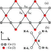
Figure 1: [color online] (a) A schematic diagram of the kagomé staircase structure as reduced to 2D in the $a$-$c$ plane. The cobalt ions are represented by open and solid circles for spine (M1) and cross-tie sites (M2), respectively. Chains of spine sites running parallel to the $a$-direction are alternatively above ($\odot$) and below the plane ($\otimes$). (b) The basis used in the linear spin-wave theory calculation.

One member of this family, Ni₃V₂O₈ (NVO), undergoes a series of phase transitions on lowering temperature Kenzelmann ; Lawes ; Wilson2 ; Rogado ; Lancaster . A very interesting characteristic of this compound is that it exhibits simultaneous ferroelectric and incommensurate AFM order, that is, multiferroic behaviour, in one of its ordered phases. In isostructural Co₃V₂O₈ (CVO), the $S=1$ magnetic moments at the Ni²⁺ site are replaced with $S=3/2$ Co²⁺ moments. CVO also displays a rich low temperature phase diagram, which has been studied using polarized and unpolarized neutron diffraction, dielectric measurements Chen , magnetization and specific heat measurements Szymczak . There is a series of four AFM ordered phases below $T_{N}=11.3$ K which can be characterized by incommensurate or commensurate ordering wavevectors $(0\tau 0)$. In contrast to NVO, the ultimate ground state in CVO is ferromagnetic and the Curie temperature is $T_{C}\sim 6$ K. Earlier powder neutron diffraction measurements Chen on CVO showed ordered magnetic moments of 2.73(2) and 1.54(6) $\mu_{B}$ on the spine and cross-tie sites, respectively, at 3.1 K. All moments are aligned along the $a$-axis direction.

While much work has been performed on the phase diagrams of NVO and CVO, little is known about the excitations and, correspondingly, the underlying microscopic spin Hamiltonian for these topical magnets. The ferromagnetic state in CVO is an excellent venue for such a study, as the ground state itself is very simple and therefore the excitations out of the ground state should be amenable to modeling. In this Letter we report inelastic neutron scattering (INS) measurements of the spin-wave excitations within the kagomé staircase plane in the FM ground state of single crystal CVO. These measurements are compared with linear spin wave theory which shows a surprising sublattice dependence to the exchange interactions.

A large (5 g) and high-quality single crystal of CVO was grown using an optical floating-zone image furnace Szymczak . Thermal INS measurements were performed at the Canadian Neutron Beam Centre at the Chalk River Laboratories using the C5 triple-axis spectrometer. A pyrolytic graphite (PG) vertically-focusing monochromator and flat analyzer were used. Measurements were performed with a fixed final neutron energy of $E_{f}=13.7$ meV and a PG filter in the scattered beam. The collimation after the monochromator was 29’-34’-72’ resulting in an energy resolution of 0.9 meV FWHM.

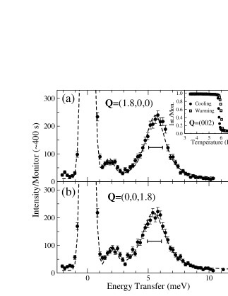
Figure 2: Representative constant-Q INS spectra with (a) Q$=(1.8,0,0)$ and (b) Q$=(0,0,1.8)$ at $T=3$ K (FM phase). The broken line shows the resolution-corrected fits to the data, as described in the text. The solid horizontal bars indicate the instrumental energy resolution. The inset shows heating and cooling scans of the (mainly) magnetic elastic (002) Bragg scattering, characteristic of the FM ground state in CVO.

The crystal was oriented with the $(h0\ell)$ kagomé staircase plane coincident with the scattering plane. Constant-Q energy scans were performed along the high symmetry $(h00)$ and $(00\ell)$ directions in this plane. Figures 2 (a) and (b) show representative constant-Q scans at $T=3$ K and Q=(1.8, 0, 0) and (0, 0, 1.8), respectively. The (002) nuclear Bragg peak is very weak, and is coincident with a strong FM Bragg peak below $T_{C}$. The inset of Fig. 2(a) shows the temperature dependence of this Bragg reflection on independent warming and cooling runs. An abrupt falloff in intensity near $T_{C}\sim 6$ K and accompanying hysteresis indicate the strongly discontinuous nature of this phase transition.

The overall features of the two spectra in Fig. 2 are quantitatively similar at $T=3$ K. Two spin-wave excitations, identified on the basis of their temperature and $Q$-dependencies, are observed and have been modelled using resolution-convoluted damped harmonic oscillator (DHO) lineshapes shirane . The resulting fits are shown as the dashed lines in Fig. 2, and this analysis allows us to conclude that the higher-energy spin wave, near 5.7 meV in both cases, has a substantial intrinsic energy width of $\Gamma$=0.70(8) meV at Q=$(1.8,0,0)$ and $0.90(8)$ meV at Q=$(0,0,1.8)$.

A series of constant-Q scans for $(h00)$ and $(00\ell)$ directions were collected at $T=3$ K and are presented as a color contour map in Figs. 3 (a) and (c). Dispersive features corresponding to two bands of spin waves are seen in both data sets. The top of the upper spin-wave band at $\Delta E\sim 5.7$ meV corresponds to excitations reported earlier using a time-of-flight technique Wilson2 . These constant-Q scans were fit to resolution-convoluted DHO lineshapes, which gave intrinsic energy widths for the higher-energy spin-wave mode at all wavevectors ranging from $\Gamma=0.6$ to 1.1 meV, while the lower-energy spin waves were resolution limited at all wavevectors. This indicates a finite lifetime for the higher-energy spin waves even at temperatures $\sim T_{C}/2$.

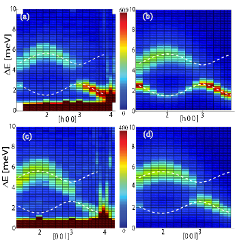
Figure 3: Color contour maps of INS at $T=3$ K [(a) and (c)] and corresponding linear spin-wave theory [(b) and (d)] as described in the text. The broken lines show the dispersion relations resulting from this spin-wave theory analysis.

The spin-wave spectrum evolves rapidly with increasing temperature. Figure 4 (a) shows ${\bf Q}=(3.4,0,0)$ scans at $T=3$ K (FM phase) and $T=20$ K [well into the paramagnetic (PM) phase]. In the FM phase there is a prominent spin-wave peak at $\Delta E=2.0$ meV. A higher energy spin-wave peak is also present in this scan but with a much lower peak intensity and an intrinsic energy width of $\Gamma=0.9$ meV. At 20 K the well-defined low-energy spin wave has disappeared and only broad low-$\Delta E$ scattering remains. The inset of Fig. 4 (a) shows the temperature dependence of spin wave peak intensity at $\Delta E=2.0$ meV in the neighborhood of $T_{C}$. The same rapid falloff as was seen in the magnetic Bragg scattering at $(002)$ is seen in the inelastic intensity, as well as the same hysteresis, indicating that these spin waves are strongly coupled to the ferromagnetic order parameter.

Figure 4 (b) shows the same constant-Q scans as in Fig. 2 but now at 20 K rather than 3 K. The well-defined spin-wave modes are no longer present, and the low-energy inelastic scattering is significantly greater at ${\bf Q}$=$(0,0,1.8)$ as compared with $(1.8,0,0)$ at $T=20$ K. The temperature dependence of this scattering is contrasted in the inset of Fig. 4 (b). The Q=$(1.8,0,0)$ inelastic scattering drops quickly at $T_{C}\sim 6$ K while that at Q= $(0,0,1.8)$ gradually increases with temperature. We attribute this difference to prominent longitudinal easy-axis spin fluctuations along the $a$-axis at high temperatures. Given that the neutron scattering cross-section shirane is sensitive to magnetic fluctuations perpendicular to Q, longitudinal fluctuations would be seen in the Q=$(0,0,1.8)$ spectrum rather than the $(1.8,0,0)$ spectrum. Note that the highest temperature transition, to the paramagnetic state at $T_{N}=11.3$ K, is evident as a change in slope of the temperature dependence shown in the inset of Fig. 4 (b), and both $T_{C}\sim 6$ K and $T_{N}=11.3$ K are indicated by dashed vertical lines in this inset.

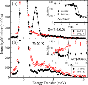
Figure 4: [color online] (a) INS scans at ${\bf Q}=(3.4,0,0)$ for $T=3$ K and $T=20$ K. The inset shows the temperature dependence of the scattering at the inelastic peak position. The lines are guides to the eye. (b) Scans in the PM phase for ${\bf Q}=(1.8,0,0)$ and ${\bf Q}=(0,0,1.8)$. The inset (same legend as main figure) shows the temperature dependence of the inelastic scattering at the spin-wave peak (for $T=3$ K, see Fig. 2) at $\Delta E=1.86$ meV for the different $\bf{Q}$ directions. The vertical dotted lines in the inset indicate $T_{C}$ and $T_{N}$.

We have carried out a linear spin-wave theory analysis of the magnetic excitations observed in Figs. 3 (a) and (c) to understand as much of the relevant microscopic spin Hamiltonian as possible. The full Hamiltonian is potentially complicated if account is taken of the two inequivalent magnetic sites and the 3D kagomé staircase structure. We employed a 2D model in which the magnetic ions in a layer are projected onto the average plane of the layer (Fig. 1) and only near-neighbor exchange and single-ion anisotropy are included.

We change from the conventional centered-rectangular unit cell to a primitive rhombohedral unit cell defined by lattice vectors ${\bf R}_{1}=(\frac{a}{2},\frac{c}{2})$ and ${\bf R}_{2}=(\frac{a}{2},-\frac{c}{2})$ and basis vectors $\delta$${}_{1}={\bf R}_{1}/2$, $\delta$${}_{2}={\bf R}_{2}/2$, and $\delta$${}_{3}=\mbox{\boldmath$0$}$. If ${\bf R}$ describes the set of lattice points and ${\bf S}_{\bf r}$ is the spin operator at a location r we can write

$${\cal H}_{sc} = -J_{sc}\sum_{\bf R}\sum_{\mbox{\boldmath${\scriptstyle\delta}$}=\pm\mbox{\boldmath${\scriptstyle\delta}$}_{1},\pm\mbox{\boldmath${\scriptstyle\delta}$}_{2}}{\bf S}_{\bf R}\cdot{\bf S}_{{\bf R}+{\mbox{\boldmath${\scriptstyle\delta}$}}},$$ (1)

$${\cal H}_{ss} = -J_{ss}\sum_{\bf R}\big{[}{\bf S}_{{\bf R}+\mbox{\boldmath${\scriptstyle\delta}$}_{1}}\!\cdot\!{\bf S}_{{\bf R}-\mbox{\boldmath${\scriptstyle\delta}$}_{2}}+{\bf S}_{{\bf R}-\mbox{\boldmath${\scriptstyle\delta}$}_{1}}\!\cdot\!{\bf S}_{{\bf R}+\mbox{\boldmath${\scriptstyle\delta}$}_{2}}\big{]}.$$ (2)

${\cal H}_{sc}$ and ${\cal H}_{ss}$ are the exchange interactions between spine and cross-tie spins with couplings $J_{sc}$ and $J_{ss}$. The fact that the spine and cross-tie spins are found to be ferromagnetically aligned implies that $J_{sc}$ is positive. We choose the spin $z$-axis parallel to the crystallographic $a$-axis, consistent with the ordered moment direction. Magnetization measurements have established that the crystallographic $b$-axis (spin $x$-axis) is a harder axis than the $c$-axis (spin $y$-axis) Szymczak . The appropriate single-ion anisotropy Hamiltonian, ${\cal H}_{a}$, distinguishes the three orthogonal directions and the inequivalent sites

$${\cal H}_{a}=\sum_{\bf R}\sum_{i=1,2,3}\sum_{\alpha=x,y,z}A_{i}^{\alpha}(S^{\alpha}_{{\bf R}+\mbox{\boldmath${\scriptstyle\delta}$}_{i}})^{2}.$$ (3)

The sequence from hard to easy axis is established by the condition $A_{i}^{x}>A_{i}^{y}>A_{i}^{z}$. We use reduced anisotropies: $\Delta_{i}=(A_{i}^{x}+A_{i}^{y}-2A_{i}^{z})/2$ and $\epsilon_{i}=(A_{i}^{x}-A_{i}^{y})/2$. Since the $i=1$ and $i=2$ sites are equivalent there are 4 independent parameters $\Delta_{s}$, $\Delta_{c}$, $\epsilon_{s}$, and $\epsilon_{c}$.

In linear spin-wave theory holstein the total Hamiltonian ${\cal H}$ may be written in term of spin-wave operators $c_{i}({\bf k})$ and $c^{\dagger}_{i}({\bf k})$

$${\cal H}=\sum_{{\bf k},i,j}h_{ij}({\bf k})c^{\dagger}_{i}({\bf k})c_{j}({\bf k})\ +\frac{1}{2}\sum_{{\bf k},i,j}g_{ij}({\bf k})\left(c^{\dagger}_{i}({\bf k})c^{\dagger}_{j}(-{\bf k})+c_{j}(-{\bf k})c_{i}({\bf k})\right),$$ (4)

$$h({\bf k})=2S\left(\begin{array}[]{ccc}J_{sc}+J_{ss}+\Delta_{s}&-J_{ss}\cos{\bf k}\cdot(\mbox{\boldmath$\delta$}_{1}+\mbox{\boldmath$\delta$}_{2})&-J_{sc}\cos{\bf k}\cdot\mbox{\boldmath$\delta$}_{1}\\ -J_{ss}\cos{\bf k}\cdot(\mbox{\boldmath$\delta$}_{1}+\mbox{\boldmath$\delta$}_{2})&J_{sc}+J_{ss}+\Delta_{s}&-J_{sc}\cos{\bf k}\cdot\mbox{\boldmath$\delta$}_{2}\\ -J_{sc}\cos{\bf k}\cdot\mbox{\boldmath$\delta$}_{1}&-J_{sc}\cos{\bf k}\cdot\mbox{\boldmath$\delta$}_{2}&2J_{sc}+\Delta_{c}\end{array}\right),\qquad g({\bf k})=2S\left(\begin{array}[]{ccc}\epsilon_{s}&0&0\\ 0&\epsilon_{s}&0\\ 0&0&\epsilon_{c}\\ \end{array}\right),$$ (11)

where $i,j=1,2,3$. Although the moments on the different sites are unequal we make the simplifying assumption that $S=3/2$ for all sites.

The unpolarized magnetic neutron scattering cross-section and the spin-spin correlation functions it contains can be related to one spin-wave Green’s functions. The Green’s functions can be calculated by inverting a matrix involving the two matrices, $h({\bf k})$ and $g({\bf k})$ defined above, following Coll and Harris coll . The spin-wave energies are determined by solving for the zeros of a determinant involving matrix elements of the inverse Green’s function. The resulting scattering function ${\cal S}({\bf Q},\Delta E)$ for Q parallel to $(00\ell)$ is proportional to

$${\cal S}({\bf Q},\Delta E)\!\propto\!\sum_{i,j}\mbox{Im}\!\left[(h\!-\!g)(z^{2}I\!-\!h^{2}\!+\!g^{2}\!+\!hg\!-\!gh)^{-1}\right]_{i,j}$$ (12)

where $I$ is the identity matrix, $\bf{k}=\bf{Q}$ and $z=\Delta E-i\Gamma$ is the complex energy, and $i$ and $j$ are summed over the indices of the $3\times 3$ matrix in square brackets. The expression for Q parallel to $(h00)$ has a similar form. The resulting scattering functions are multiplied by the magnetic form factor, the Bose factor, and a single intensity scale factor, and are plotted in Fig. 3 (b) and (d).

Best agreement between the experimental data and the spin-wave theory calculation in Fig. 3 was obtained for magnetic coupling predominantly between the spine and cross-tie Co ions with $J_{sc}=1.25\pm 0.08$ meV, while the spine-spine coupling $J_{ss}$ vanishes. The best fit spin-wave uniaxial anisotropy parameters are $\Delta_{s}=1.5\pm 0.1$ meV, $\Delta_{c}=2.13\pm 0.2$ meV, $\epsilon_{s}=0.6\pm 0.3$ meV, and $\epsilon_{c}=1.2\pm 0.3$ meV.

Figure 3 shows that the spin-wave theory gives a very good description of the dispersion of the two modes (dashed lines) and accounts for the observed trend of the spin waves to trade intensity as a function of $\bf{Q}$. This description is not perfect, however. The calculated dispersion of the lower spin-wave band is low compared with experiment near (200) and (002) where the intensity is very weak. The calculation is not convolved with the instrumental resolution; instead the energy width is manually set in both high and low-energy bands to correspond to the measured width. The broad (in energy) neutron groups corresponding to the upper spin-wave bands are most evident near $(200)$ and $(002)$. The lower energy spin-wave band becomes much more intense near the zone centers of $(400)$ and $(004)$. Steep excitation branches near (400) and (004) with comparitively weak intensity in the experimental data [Figs. 3 (a) and (c)] are identified as acoustic phonons with a speed of sound of $1050\pm 100$ m/s, in both directions.

To conclude, our INS study of the spin-wave excitations in the ferromagnetic ground state of CVO within its kagomé staircase plane reveal two separate spin-wave bands between 1.6 and 5.7 meV. The upper spin-wave band is damped with finite energy widths $\Gamma$ in the range of 0.6 to 1.1 meV. These spin-wave excitations can be accurately described by a simple model Hamiltonian and linear spin-wave theory. The model gives a magnetic coupling that is predominantly between the spine and cross-tie sites of the kagomé staircase.

References

- (1) Frustrated Spin Systems, edited by H.T. Diep (World Scientific Publishing Co. Pte. Ltd., Singapore, 2004).
- (2) S.T. Bramwell and M.J.P. Gingras, Science 294, 1495 (2001).
- (3) T. Kimura et al., Nature 426, 55 (2003); Nicola A. Hill, J. Phys. Chem. B 104, 6694 (2000).
- (4) K. Matan, D. Grohol, D.G. Nocera, T. Yildirim, A.B. Harris, S.H. Lee, S.E. Nagler, and Y.S. Lee, Phys. Rev. Lett. 96, 247201 (2006); D. Grohol, K. Matan, J.H. Cho, S.H. Lee, J.W. Lynn, D.G. Nocera, and Y.S. Lee, Nature Materials 4, 323 (2005).
- (5) J.S. Helton, K. Matan, M.P. Shores, E.A. Nytko, B.M. Bartlett, Y. Yoshida, Y. Takano, A. Suslov, Y. Qiu, J.-H. Chung, D.G. Nocera, and Y.S. Lee, Phys. Rev. Lett. 98, 107204 (2007).
- (6) E.E. Sauerbrei, R. Faggiani and C. Calvo, Acta Cryst.B. (1973) 29, 2304.
- (7) M. Kenzelmann, A.B. Harris, A. Aharony, O. Entin-Wohlman, T. Yildirim, Q. Huang, S. Park, G. Lawes, C. Broholm, N. Rogado, R.J. Cava, K.H. Kim, G. Jorge, and A.P. Ramirez, Phys. Rev. B 74, 014429 (2006).
- (8) G. Lawes, M. Kenzelmann, N. Rogado, K.H. Kim, G.A. Jorge, R.J. Cava, A. Aharony, O. Entin-Wohlman, A.B. Harris, T. Yildirim, Q.Z. Huang, S. Park, C. Broholm, and A.P. Ramirez, Phys. Rev. Lett. 93, 247201, (2004).
- (9) N.R. Wilson, O.A. Petrenko, G. Balakrishman, P. Manuel, and B. Fak, J. Magn. and Magn. Mat. 310, 1334 (2007).
- (10) N. Rogado, G. Lawes, D.A. Huse, A.P. Ramirez, and R.J. Cava, Solid State Comm. 124, 229 (2002).
- (11) T. Lancaster, S.J. Blundell, P.J. Baker, D. Prabhakaran, W. Hayes, and F.L. Pratt, Phys. Rev. B 75, 064427 (2007).
- (12) Y. Chen, J.W. Lynn, Q. Huang, F.M. Woodward, T. Yildirim, G. Lawes, A.P. Ramirez, N. Rogado, R.J. Cava, A. Aharony, O. Entin-Wohlman, and A.B. Harris, Phys. Rev. B 74, 014430 (2006).
- (13) R. Szymczak, M. Baran, R. Diduszko, J. Fink-Finowicki, M. Gutowska, A. Szewczyk, and H. Szymczak, Phys. Rev. B 73, 094425 (2006).
- (14) G. Shirane, S.M. Shapiro, and J.M. Tranquada, Neutron Scattering with a Triple-Axis Spectrometer, (Cambridge University Press, Cambridge, 2002) p.47.
- (15) T. Holstein and H. Primakoff, Phys. Rev. 58, 1098 (1940).
- (16) C.F. Coll III and A.B. Harris, Phys. Rev. B 4, 2781 (1971).