An ACS Survey of Globular Clusters V: Generating a Comprehensive Star Catalog for Each Cluster

Abstract

The ACS Survey of Globular Clusters has used HST’s Wide-Field Channel to obtain uniform imaging of 65 of the nearest globular clusters to provide an extensive homogeneous dataset for a broad range of scientific investigations. The survey goals required not only a uniform observing strategy, but also a uniform reduction strategy. To this end, we designed a sophisticated software program to process the cluster data in an automated way. The program identifies stars simultaneously in the multiple dithered exposures for each cluster and measures them using the best available PSF models. We describe here in detail the program’s rationale, algorithms, and output. The routine was also designed to perform artificial-star tests, and we run a standard set of $\sim$10⁵ tests for each cluster in the survey. The catalog described here will be exploited in a number of upcoming papers and will eventually be made available to the public via the world-wide web.

KEYWORDS: Globular clusters: general — catalogs — techniques: image processing, photometric

1 INTRODUCTION

The Galaxy’s globular clusters hold important clues to a large number of scientific questions, ranging from star formation to stellar structure, galaxy evolution, and cosmology. Many of these questions can be answered only by surveying a significant fraction of the clusters and studying the cluster system as an ensemble. Initial globular cluster surveys (e.g., Zinn 1980, Armandroff 1989) focused on integrated-light properties such as total brightness, colors, metallicity, and reddening. Many subsequent “surveys” have been constructed by assembling various data from the multitude of independent observations of individual clusters (e.g., Djorgovski & King 1986, Djorgovski & Meylan 1993, Trager et al. 1995, Lee et al. 1996, and Harris 1996). However, since each cluster is typically observed with a different instrument and under different conditions, there are limits to how homogeneous such a patched-together data set can be.

In an effort to construct a more homogeneous sample, Rosenberg et al. (2000a, 2000b) surveyed 56 clusters from the ground, producing star catalogs and color-magnitude diagrams (CMDs) that can be directly intercompared to yield relative ages and relative horizontal-branch morphologies. Piotto et al. (2002) used WFPC2 snapshots to image the central regions of 74 clusters and construct CMDs in a uniform photometric system. These surveys have allowed clusters to be studied on a more even footing than ever before, but the data in these surveys still suffer from severe crowding in the cluster cores, irregularities in the sampling, and gaps in the field of view. Thanks to its fine sampling, large dynamic range and wide, contiguous field of view, the Advanced Camera for Survey’s (ACS’s) Wide-Field Channel (WFC) on board the Hubble Space Telescope (HST) is the first instrument that can improve dramatically on all of these shortcomings.

The ACS Survey of Globular Clusters presented here was designed to provide a nearly complete catalog of all the stars present in the central two arcminutes of 65 targeted clusters. Such a uniform data set has many scientific applications, and we are currently in the process of using the catalog for broad studies of: binary-star distributions, absolute and relative ages, horizontal-branch morphology, blue stragglers, isochrone fitting, mass functions, and dynamical models. We are also measuring internal motions and orbits for those clusters that have sufficient archival data. In addition to addressing these major scientific issues, one of the main legacies of this survey will be to provide the community with a definitive catalog of stars in the central regions of these clusters. This data base will serve as a touchstone for studies of these clusters for many years to come, and as such it should be as accurate and comprehensive as possible.

The images that make up this survey consist almost entirely of point sources, but each cluster has a different central concentration and density profile. So, to construct a definitive catalog, we needed a star-finding and measuring routine that works in a variety of crowding situations, often across the same cluster field. With this in mind, we developed a sophisticated computer program that simultaneously analyzes all of the survey exposures for each cluster (one short exposure plus four to five deep exposures for each of the F606W and F814W filters), to construct a single list of detected stars and their measured parameters. The routine was designed to deal well with both crowded and uncrowded situations, and as such it is able to find almost every star that a human could find. At the same time, the routine uses the independence of the pointings and knowledge of the PSF to avoid including image artifacts in the list.

This paper describes the data-reduction procedure we developed and the resulting catalog we produced for each cluster. It is organized as follows: We begin by describing the observations we have available for each cluster (§ 2) and the preliminary set-up steps required before the finding program could be run on the images (§ 3). Before diving into the details of our procedures, we first give an overview of the general considerations that are involved in finding and measuring stars in dithered, undersampled images of globular clusters (§ 4). We then describe in detail our automated finding and measuring program and use it to construct a catalog of the real stars for each cluster (§ 5). We use the same program to perform a standard battery of artificial-star tests for each cluster (§ 6). We also consider the photometric errors that are present in an ACS data set such as that collected here (§ 7). Finally, we describe the photometric and astrometric calibration and the assembly of the final catalog of positions, magnitudes, quality characterizations, etc., for the detected stars for each cluster field (§ 8). We end with a summary of upcoming scientific results and additional studies that will complement this survey (§ 9).

2 OBSERVATIONS

The goal of the ACS Survey of Globular Clusters (GO-10775, PI-Sarajedini) was to image the central regions of a large number of globular clusters in order to generate a homogeneous set of star catalogs. The clusters are all at different distances and all have different central densities and radial profiles, so there is of course no way to obtain identical data for every cluster, but our aim was to come as close to this ideal as possible.

Each cluster was observed for one orbit in F606W ($V$) and one orbit in F814W ($I$), except for M54, which was observed for 2 orbits in each filter. In each orbit, we took one short exposure and either four or five deeper exposures, depending on how many we could fit into the orbit. We chose the exposure times for each cluster so that the horizontal-branch stars would be unsaturated in the short exposure and the turn-off and subgiant branch stars would be unsaturated in the deep exposures. For the typical cluster, we reach about 6 magnitudes below the turn-off, to about 0.2 $M_{\odot}$. Table 1 provides the details of our observations for each cluster.

Table 1: Summary of cluster observations. All observations were taken in 2006.

Cluster	Dataset	Date	RA	Dec	PA_V3	F606W	F814W
Arp2	j9l925	4/22	19:28:44	$-$30:21:14	83.24	40s, 5x345s	40s, 5x345s
E3	j9l906	4/15	09:20:59	$-$77:16:57	245.09	5s, 4x100s	5s, 4x100s
Lynga7	j9l904	4/07	16:11:02	$-$55:18:52	124.32	35s, 5x360s	35s, 5x360s
NGC0104	j9l960	3/13	00:24:05	$-$72:04:51	346.17	3s, 4x 50s	3s, 4x 50s
NGC0362	j9l930	6/02	01:03:14	$-$70:50:54	44.24	10s, 4x150s	10s, 4x170s
NGC0288	j9l9ad	7/31	00:52:45	$-$26:34:43	92.32	10s, 4x130s	10s, 4x150s
NGC1261	j9l909	3/10	03:12:15	$-$55:13:01	294.90	40s, 5x350s	40s, 5x360s
NGC1851	j9l910	5/01	05:14:06	$-$40:02:49	317.14	20s, 5x350s	20s, 5x350s
NGC2298	j9l911	6/12	06:48:59	$-$36:00:19	337.87	20s, 5x350s	20s, 5x350s
NGC2808	j9l947	3/01	09:12:02	$-$64:51:46	205.10	23s, 5x360s	23s, 5x370s
NGC3201	j9l946	3/14	10:17:36	$-$46:24:39	205.05	5s, 4x100s	5s, 4x100s
NGC4147	j9l949	4/11	12:10:06	$+$18:32:31	343.98	50s, 5x340s	50s, 5x340s
NGC4590	j9l932	3/07	12:39:27	$-$26:44:33	142.48	12s, 4x130s	12s, 4x150s
NGC4833	j9l931	6/02	12:59:34	$-$70:52:29	296.05	10s, 4x150s	10s, 4x170s
NGC5024	j9l950	3/02	13:12:55	$+$18:10:08	77.47	45s, 5x340s	45s, 5x340s
NGC5053	j9l902	3/06	13:16:27	$+$17:41:52	73.41	30s, 5x340s	30s, 5x350s
NGC5139	j9l9a7	7/22	13:26:45	$-$47:28:36	290.54	4s, 4x 80s	4s, 4x 90s
NGC5272	j9l953	2/20	13:41:11	$+$28:22:31	81.00	12s, 4x130s	12s, 4x150s
NGC5286	j9l912	3/03	13:46:26	$-$51:22:23	133.74	30s, 5x350s	30s, 5x360s
NGC5466	j9l903	4/12	14:05:27	$+$28:32:04	20.07	30s, 5x340s	30s, 5x350s
NGC5904	j9l956	3/13	15:18:33	$+$02:04:57	92.14	7s, 4x140s	7s, 4x140s
NGC5927	j9l914	4/13	15:28:00	$-$50:40:22	138.13	30s, 5x350s	25s, 5x360s
NGC5986	j9l915	4/16	15:46:03	$-$37:47:09	126.51	20s, 5x350s	20s, 5x350s
NGC6093	j9l916	4/09	16:17:02	$-$22:58:30	101.42	10s, 5x340s	10s, 5x340s
NGC6101	j9l917	5/31	16:25:48	$-$72:12:06	181.91	35s, 5x370s	35s, 5x380s
NGC6121	j9l964	3/05	16:23:35	$-$26:31:31	99.90	1.5s, 2x 25s,	1.5s, 4x 30s
						2x 30s
NGC6144	j9l943	4/15	16:27:14	$-$26:01:29	103.41	25s, 5x340s	25s, 5x350s
NGC6171	j9l933	3/30	16:32:31	$-$13:03:12	93.29	12s, 4x130s	12s, 4x150s
NGC6205	j9l957	4/02	16:41:41	$+$36:27:36	66.23	7s, 4x140s	7s, 4x140s
NGC6218	j9l944	3/01	16:47:14	$-$01:56:51	97.68	4s, 4x 90s	4s, 4x 90s
NGC6254	j9l962	3/05	16:57:08	$-$04:05:57	96.12	4s, 4x 90s	4s, 4x 90s
NGC6304	j9l918	4/14	17:14:32	$-$29:27:44	98.88	20s, 5x340s	20s, 5x350s

Cluster	Dataset	Date	RA	Dec	PA_V3	F606W	F814W
NGC6341	j9l958	4/11	17:17:07	$+$43:08:11	62.25	7s, 4x140s	7s, 4x150s
NGC6352	j9l959	4/10	17:25:29	$-$48:25:22	105.79	7s, 4x140s	7s, 4x150s
NGC6362	j9l934	5/30	17:31:54	$-$67:02:53	106.79	10s, 4x130s	10s, 4x150s
NGC6366	j9l907	3/30	17:27:44	$-$05:04:36	87.53	10s, 4x140s	10s, 4x140s
NGC6388	j9l919	4/06	17:36:17	$-$44:44:06	100.71	40s, 5x340s	40s, 5x350s
NGC6397	j9l965	5/29	17:40:41	$-$53:40:24	148.54	1s, 4x 15s	1s, 4x 15s
NGC6441	j9l951	5/28	17:50:12	$-$37:03:04	122.48	45s, 5x340s	45s, 5x350s
NGC6496	j9l9a9	5/31	17:59:03	$-$44:15:58	134.74	30s, 5x340s
	j9l920	4/01	17:59:03	$-$44:15:58	94.46		30s, 5x350s
NGC6535	j9l935	3/30	18:03:50	$-$00:17:48	86.04	12s, 4x130s	12s, 4x150s
NGC6541	j9l936	4/01	18:08:02	$-$43:42:57	92.60	8s, 4x140s	8s, 4x150s
NGC6584	j9l921	5/27	18:18:37	$-$52:12:54	131.18	25s, 5x350s	25s, 5x360s
NGC6624	j9l922	4/14	18:23:40	$-$30:21:39	90.06	15s, 5x350s	15s, 5x350s
NGC6637	j9l937	5/22	18:31:23	$-$32:20:53	99.28	18s, 5x340s	18s, 5x340s
NGC6652	j9l938	5/27	18:35:45	$-$32:59:24	101.82	18s, 5x340s	18s, 5x340s
NGC6656	j9l948	4/01	18:36:24	$-$23:54:12	86.47	3s, 4x 55s	3s, 4x 65s
NGC6681	j9l939	5/20	18:43:12	$-$32:17:30	96.43	10s, 4x140s	10s, 4x150s
NGC6715	j9l923	5/25	18:55:03	$-$30:28:41	94.18	2x30s,	2x30s,
						10x340s	10x350s
NGC6717	j9l940	3/29	18:55:06	$-$22:42:03	84.61	10s, 4x130s	10s, 4x150s
NGC6723	j9l941	6/02	18:59:33	$-$36:37:54	106.02	10s, 4x140s	10s, 4x150s
NGC6752	j9l966	6/24	19:10:52	$-$59:59:04	119.42	2s, 4x 35s	2s, 4x 40s
NGC6779	j9l905	5/11	19:16:35	$+$30:11:05	59.22	20s, 5x340s	20s, 5x350s
NGC6809	j9l963	4/19	19:39:59	$-$30:57:44	81.46	4s, 4x 70s	4s, 4x 80s
NGC6838	j9l9a8	5/12	19:53:46	$+$18:46:42	65.46	4s, 4x 75s	4s, 4x 80s
NGC6934	j9l927	3/31	20:34:11	$+$07:24:15	89.61	45s, 5x340s	45s, 5x340s
NGC6981	j9l942	5/17	20:53:27	$-$12:32:12	72.88	10s, 4x130s	10s, 4x150s
NGC7078	j9l954	5/02	21:29:58	$+$12:10:01	77.40	15s, 4x130s	15s, 4x150s
NGC7089	j9l952	4/16	21:33:26	$-$00:49:23	78.04	20s, 5x340s	20s, 5x340s
NGC7099	j9l955	5/02	21:40:22	$-$23:10:45	69.63	7s, 4x140s	7s, 4x140s
Pal1	j9l901	3/17	03:33:23	$+$79:34:50	236.85	15s, 5x390s	15s, 5x390s
Pal2	j9l908	8/08	04:46:06	$+$31:22:51	87.56	5x380s	5x380s
Pal12	j9l928	5/21	21:46:38	$-$21:15:03	63.70	60s, 5x340s	60s, 5x340s
Terzan7	j9l924	6/03	19:17:43	$-$34:39:27	99.90	40s, 5x345s	40s, 5x345s
Terzan8	j9l926	6/03	19:41:44	$-$34:00:01	95.01	40s, 5x345s	40s, 5x345s

To give the survey as much spatial uniformity as possible, we stepped our observations so that no star would fall in the inter-chip gap in more than one of the deep exposures. Since the WFC field-of-view is actually quite rhombus-shaped, we also made sideways steps so that the resulting field would be as square as possible. Figure 1 shows the coverage for a typical cluster that had four deep exposures.

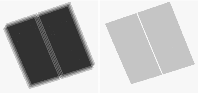
Figure 1: Left: the depth of the deep stack in the case of four deep images. Most parts of the field are covered by all four images. We dithered the observations to ensure that a star will fall in the gap in at most one deep exposure; hence we have at least three images covering all areas but the very edges. Right: the depth of the short stack (1 or 0). Some bright stars will fall in the gap of the short-exposure image and can be measured (albeit poorly) only in the deep exposures.

3 PRELIMINARY SET-UP

The HST pipeline generates two main types of output image. The flt images have been flat-fielded and bias-subtracted, but are otherwise left in the raw WFC CCD frame, which suffers from a lot of distortion. The standard pipeline also generates a drz image for each set of associated exposures. This is a drizzled, composite image of all the exposures that were taken in the same visit through the same filter. The drz images have been resampled into a standard distortion-free frame and tied to an absolute astrometric frame via the guide stars. A careful photometric calibration has also been worked out for them (Sirianni et al. 2005). Thus, the drz images can serve to establish both our astrometric reference frame and photometric zero points. However, because they have been resampled, they are not well suited for high-accuracy PSF-fitting analysis. For this reason, we used the drz images for calibration, but our final measurements came from careful analysis of the individual flt images.

The first step in reducing the data for each cluster was to construct a reference frame and relate each flt exposure to this frame, both astrometrically and photometrically.

3.1 Constructing a reference frame for each cluster

To construct an astrometric frame for each cluster, we first measured simple centroid positions for the bright, isolated stars in the F606W drz image. Using the WCS header information, we converted these positions into a reference frame that has the targeted cluster center at coordinate [3000,3000], the $y$ axis aligned with North, and a scale of 50 mas/pixel. For all cluster orientations, this allows the entire observed field to fit conveniently within a frame that is 6000$\times$6000 pixels.

The next step was to relate each of the individual flt exposures to this reference frame. We started by measuring positions and fluxes for all of the reasonably bright stars in each flt exposure with the program img2xym_WFC.09x10, documented in Anderson & King (2006, AK06). Briefly, the program starts with a library PSF, which was constructed empirically for each filter using GO-10424 observations of the outskirts of NGC 6397. These library PSFs account for the spatial variations in the WFC PSF due to the telescope optics and the variable charge diffusion present in the CCD (see Krist 2005). The PSF in each exposure can differ from this library PSF due to spacecraft breathing or focus changes, so we fitted the library PSF to bright stars in each image and came up with a spatially constant perturbation to the PSF that better represents the star images in each individual exposure. Using the improved PSF, the program then went through each exposure and measured positions and fluxes for the bright, isolated stars. The exposure-specific, improved PSFs were saved for later in the analysis.

We next found the common stars between the reference list and the star list for each exposure. This allowed us to define a general, 6-parameter linear coordinate transformation from the distortion-corrected frame of each exposure into the reference frame. Since the photometry and astrometry are more accurately measured in the flt frames than in the drz frame, we improved the internal quality of the reference frame by iteration. The final reference-frame positions and fluxes for the bright stars should be internally accurate to better than 0.01 pixel and 0.01 magnitude.

Using this reference list of stars for each cluster, we computed the final astrometric transformations and photometric zero points from each short and deep exposure into the reference frame. The photometric system at this stage was kept in instrumental magnitudes, $-2.5\,{\rm log}_{10}({\rm flux}_{\rm DN})$, where the flux corresponds to that measured in the deep flt images for the cluster at hand. It was convenient to keep our photometry in this instrumental system until calibration at the very end (§ 8.3), because instrumental magnitudes make it easier to assess errors in terms of the expected signal to noise.

3.2 Stack construction

The transformations from the individual exposures into the reference frame allowed us to construct a stacked representation of each field. We did not use these stacks in the quantitative analysis, but they were an invaluable tool which enabled us to inspect star lists and evaluate the star-finding algorithm. (It is worth noting that the drz images which were produced in the ACS pipeline were not adequate for this for several reasons: [1] the pipeline uses the commanded POS-TARGs to register the exposures in a common frame, whereas our empirical star-based transformations allow a much more accurate mapping from the exposures into the reference frame; [2] the pipeline is set up to deal with an arbitrary set of images with different exposure times, whereas our stacking algorithm could be optimized for the 3 to 5 deep exposures plus one shallow exposure that we have for each filter; and [3] we wanted the image to be in our reference frame, but did not want to resample the drz image and thus degrade the resolution even further.)

There is no unique way to construct a stacked image from a dithered set of exposures. Our construction of the stacks was analogous to using drizzle (Fruchter & Hook 2002) with pixfrac = 0. We went through the reference frame pixel by pixel and used the inverse coordinate transformations and inverse distortion corrections to map the center of each reference-frame pixel into the frame of each of the individual F606W exposures. We then identified the closest pixel in each of the 3 to 5 exposures and computed a sigma-clipped mean of these pixel values. Finally, we set the value of the reference-frame pixel to this mean, and moved on to the next pixel in the reference frame. This produced a stack of the deep exposures.

To deal with pixels that were saturated in the deep exposures, we generated a similar stack from the short exposure (actually, a stack from just one image is better called a resampling). We then constructed a composite stack by starting with the deep-exposure stack and replacing any pixel that was within 3 pixels of a saturated pixel with the exposure-time-scaled value from the short-exposure stack. Finally, we put the WCS header information into this composite stack for each filter. Figure 2 shows an example of the stacked images for a 100$\times$100-pixel region at the center of 47 Tuc.

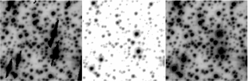
Figure 2: (Left) A 100$\times$100-pixel (5$\times$5-arcsecond) region in the stack from the deep F606W exposures of 47 Tuc; (middle) same for the short F606W exposure; (right) the combination of the long and short exposures.

We constructed such a composite stack for the F606W and the F814W exposures for each cluster. These stacks were not used directly in the reductions discussed in the next sections, but because they are a simple representation of the scene without regard to the locations of stars, they provide a critical sanity test of our finding and measuring routines. They will also serve as excellent finding charts for future spectroscopic projects.

4 GENERAL CONSIDERATIONS FOR THE FINDING AND MEASURING PROCEDURE

In the previous section, we constructed a calibrated reference frame for each cluster and found the photometric and astrometric transformation from each exposure into this frame. These transformations allowed us to construct a composite stacked image for each cluster. The next step was to construct a composite list of stars for each cluster.

Our strategy for finding and measuring stars had to be tailored to the scientific goals of the project and to the specifics of the detector and fields. In this section, we discuss some of the issues involved in constructing a catalog of stars from moderately undersampled images of globular clusters, where the stellar density can vary by orders of magnitude, and where there are both bright giants and faint main-sequence stars together in the same field. In this section, we provide an overview of the reduction; the details will be given in Section 5.

4.1 The goals of the survey

There are many different scientific objectives for this data set: luminosity-function analysis, isochrone fitting, binary studies, etc. Many of these different applications would benefit from different sampling strategies. For instance, luminosity-function (LF) studies do not require precise photometry to sift stars into 0.5-magnitude-wide bins, but LF studies do depend on high completenesses and reliable completeness corrections. On the other hand, when fitting isochrones to CMDs, we do not need a particularly complete sample of stars, but we do need a sample with the smallest possible photometric errors. In order to satisfy these competing requirements, we pursued a two-pronged strategy. Our primary goal was to identify as many stars as possible, so that no future searches would be necessary on these images. At the same time we sought to document which stars were more likely to be better measured. This way, each application can cull from the catalog the sample of stars that is best suited for the analysis at hand.

4.2 The need for automation

While we wanted our catalogs to be as comprehensive as possible, because of crowding and signal-to-noise limitations we could not hope to identify every star in every cluster field. The best we could hope for was to find all the stars that could be found by a careful human. There are hundreds of thousands of stars in many of these fields, so finding stars by hand was not very practical. Add to this the need to run artificial-star tests and it was clear that we had to come up with a completely automated finding and measuring procedure. This procedure had to: (1) be optimized for the WFC detector and globular-cluster fields, (2) find almost everything that a person would find, (3) misidentify a minimum of artifacts as stars, and (4) measure each star as accurately as possible. Below we discuss our general approach to dealing with these issues. In the next section, we will deal with the specifics.

4.3 Finding stars in undersampled images

In well-sampled images, it can be useful to convolve the image with a PSF in order to highlight the signal from the point sources over the random pixel-to-pixel noise. In undersampled images, however, much of the flux of a point source is concentrated in its central pixel. This undersampling makes it counterproductive to convolve the image before finding, because the stars already stand out as starkly as they can in the raw frames (or in frames in which the brighter stars have been subtracted out). An additional complication of undersampling is that it is often difficult to determine from a single undersampled image whether or not a given detection is stellar, so we need some independent way to establish which detections are really stars.

The best way to find stars in undersampled images, then, is to take a set of dithered exposures and look for significant local maxima (or “peaks”) that occur in the same place in the field in several independent exposures. The dithering is critical because it allows us to differentiate real sources from warm pixels or cosmic rays.

4.4 Iterative finding

The stars used in § 3.1 to relate the individual exposures to the reference frame were found with a single pass through each image. The finding routine found only stars that had no brighter neighbors within four pixels. Such an algorithm finds almost all of the bright stars in a field, but it misses many of the obvious faint stars in the wings of the bright ones. If after finding the bright stars, we were then to subtract them out and search for more stars in the subtracted images, we could both find more faint stars and at the same time improve the photometry for the brighter stars (by subtracting the fainter stars before our final measurement of the brighter ones).

There are two ways to perform such an iterative search. The first approach is to make multiple passes through the entire field. This has the advantage that it treats the field as a contiguous unit, but it is extremely memory intensive and requires maintaining many large, intermediate images (the raw images, subtracted images, model images, etc).

An alternative strategy is to reduce one patch of the field at a time, doing multiple passes on that patch before moving on to the next patch. Such a patch must be larger than the distance over which stars can influence each other, but it can be small enough to allow the transformations to be linear and to treat the PSFs as spatially constant within the patch. The patch approach also has an advantage for doing artificial-star (AS) tests. When reducing the entire field as a unit, AS tests must be done in parallel. To ensure that artificial-stars will not affect the crowding they are intended to measure, we can add at most one test star every 20$\times$20 pixels and are thus limited to about $\sim$40,000 stars per run. On the other hand, with a patch-based approach we can do AS tests in series, one after another, with no worry of them ever interfering with each other. This allows the number of tests per run to be limited only by computing time. For all these reasons, we chose to reduce each field using a mosaic of local patches. The details of this will be fleshed out in § 5.1.

4.5 Avoiding artifacts

One of the complications of studying globular clusters is that there are almost always very bright stars and very faint stars in the same field, and we want to study them both. The bright stars affect the faint stars in two ways. First, they dominate the region closest to them, making it hard to find faint stars that are too close. But the extremely bright stars also affect an even larger region around them because of the mottled wings of the PSF, which are very hard to model accurately.

To ensure that false detections, such as PSF artifacts or residuals from imperfect subtraction of bright stars, would not enter into our sample, we ended up insisting that any new stellar detection must stand above a conservative estimate of the error in the subtraction of the previously identified brighter stars. In practice, this means that there is a limit to how close to a brighter star a given fainter star can be reliably found. We determined that while such a requirement does exclude a small number of stars that could have marginally been found by hand, it does an excellent job of excluding non-stellar artifacts from the sample (see Fig. 3 and § 5.2). The region of exclusion as a function of brightness can easily be quantified by artificial-star tests.

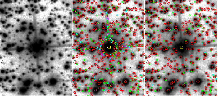
Figure 3: The stars found in a 120$\times$160-pixel region of NGC 6715 in the vicinity of a bright star. The left panel shows the scene without any stars indicated. The middle panel shows all the “stars” that would be found if we did not consider the influence of the bright star. The right panel shows the stars that were found to be bright enough to be distinct from the profile of the bright star (see § 5.2). The different colors and sizes of the circles correspond to the different passes through the data. The large yellow circles are stars that were found in the first pass. These stars are saturated in the deep exposures. The red symbols were found in the first deep-exposure pass, with the increasingly smaller green, cyan, and magenta symbols indicating stars found in subsequent passes.

4.6 Measuring stars in undersampled images

Once stars were found, we had to measure fluxes and positions for them, and our measuring algorithms also had to be tailored to the particulars of the detector and fields. Most of the signal from stars in undersampled images is concentrated in the stars’ central few pixels, so our fits clearly had to focus on those pixels.

There are two ways to measure stars in multiple exposures. We can either measure each star independently in each exposure and later combine these observations, or we can fit for a single flux and position for each star simultaneously to all the pixels in all the exposures. The first approach is generally better for bright stars, where each exposure presents a well-posed problem with an obvious stellar profile to fit. The latter approach is better for very faint stars, which cannot always be robustly found and measured in every individual exposure. In our procedures, we ended up computing the flux for each star both ways. The vast majority of stars we found were bright enough to be measured well using the first approach, so our basic catalog reports just the independently fitted fluxes. We did, however, save the simultaneous-fitted fluxes in auxiliary files.

It is worth noting that although our aim was to construct a uniform sample, it was not possible to measure all stars with the same quality. Some stars were bright and isolated and could be measured with a large, generous fitting radius. Other stars were crowded or faint, and only their core pixels could be fitted. In a sense, each star presented a special circumstance, and our general measuring algorithm had to be able to adapt as much as possible to minimize the most relevant errors for each star. The PSF provided the unifying measuring stick that enabled us to evaluate a consistent flux for all the stars, even though the fit to different stars sometimes had to focus on different pixels.

4.7 Summary of the considerations

In summary, our finding and measuring strategy had to take into account the nature of the data set and the goals of the survey. We clearly needed an automated procedure that could find stars simultaneously in multiple dithered exposures. The procedure would have to be able to use multiple iterative passes to identify faint stars in the midst of brighter ones, and it would also have to be robust against inclusion of PSF artifacts or subtraction residuals as stars. Finally, we needed to come up with a way to measure a flux and position for each star, taking into consideration its particular local environment.

5 THE REDUCTION PROGRAM

We designed a sophisticated computer program (multi_phot_WFC) that could deal with all of the above requirements in a generalized way, so that the same program could be used to reduce the data for every cluster in the sample, no matter how much crowding or saturation the cluster might suffer at its center. The program takes as input the 10 to 12 raw flt images in each cluster’s data set and the background information about how each exposure is related to the reference frame. It then analyzes the images simultaneously and outputs a list of stars that it found, including a position, $V$ and $I$ photometry, and some data-quality parameters for each star. It was set up to run in two different modes: finding real stars and running artificial-star (AS) tests. In this section we describe the mechanics of the real-star search. In § 6 we discuss the AS operation, which differs only in the set-up and the output stages.

5.1 The patch

We chose to reduce each cluster field one patch at a time, both to conserve memory and to facilitate artificial-star tests. The size of the patch was a compromise between the desire to cover as much field as possible in each patch in the real-star runs without covering too much unnecessary field in the artificial-star runs. We thus arrived at a patch size of 25$\times$25 pixels. Since stars at the edge of a patch often have significant neighbors outside of the patch, each patch allowed us to fully treat only its central 11$\times$11-pixel region. We centered a patch every 10$\times$10 pixels, so the entire 6000$\times$6000-pixel reference frame for each cluster was covered by an array of 600$\times$600 patches.

To set up each patch for analysis, we used the transformations from § 3.1 to map the location of the central pixel of the patch into each of the exposures, and extracted a local 25$\times$25-pixel raster from each exposure. We constructed a PSF model for each exposure using the appropriate library PSF for that location on the chip and the perturbation component found in § 3.1.

We also determined the linear transformation from the patch frame into the raster for each exposure. Using these transformations, we intercompared the pixels for the individual $F606W$ and $F814W$ rasters and flagged as bad any pixels that were discordant by more than $5\sigma$ with the other images for that filter. We inspected a large sample of the resulting rasters and verified that the obvious cosmic rays and warm pixels were identified. This procedure enabled us to do simultaneous fits to all the exposures without having to check each time for bad pixels.

5.2 Setting up the bright-star mask

One of the challenges in constructing a catalog from this data set was to avoid including PSF artifacts as stars. Stars brighter than an instrumental magnitude of $-12.5$ ($10^{5}$ $e^{-}$ total) often have knots and ridges in their PSFs that can be confused with stars. These features are hard to model accurately, and therefore cannot be subtracted off well. The best we could do was to conservatively estimate their contaminating influence and make sure that the stars we found stood out clearly above the bright-star halos.

To do this, we identified several bright, isolated stars that were highly saturated in the deep exposures and examined their radial profiles. Since we had a flux for each bright star from the short exposures, we could examine the radial profile for the star with a scaling matched to the PSF. Ignoring for now the diffraction spikes, we looked at the envelope of the trend with radius and drew by eye a curve that encompassed all of the obvious halo structure. Since the halo structure is largely due to scattered light, it should have the same level in F606W and F814W, though the detailed structure will be different for the different filters. Table 2 gives the upper-envelope profile we found in the $f_{\rm any}$ column.

Table 2: The profile in the vicinity of a bright star below which a fainter star is likely to be confused with a PSF artifact. Outside of the core, this is essentially a generous upper limit for the PSF as a function of radius. The PSF is normalized to have a flux of 1.0 within 10 pixels. The “any” column refers to the general radial trend, while the “spike” column tracks how the PSF intensity varies with radius along the spikes.

Radius	$f_{\rm any}$	$f_{\rm spike}$	Radius	$f_{\rm any}$	$f_{\rm spike}$
0	0.005000	0.005000	55	0.000000	0.000015
5	0.002500	0.002500	60	0.000000	0.000010
10	0.000300	0.000300	65	0.000000	0.000008
15	0.000075	0.000100	70	0.000000	0.000006
20	0.000035	0.000050	75	0.000000	0.000005
25	0.000020	0.000042	80	0.000000	0.000004
30	0.000010	0.000035	85	0.000000	0.000003
35	0.000005	0.000030	90	0.000000	0.000002
40	0.000003	0.000025	95	0.000000	0.000001
45	0.000002	0.000022	100	0.000000	0.000000
50	0.000001	0.000020

To make use of this profile, before we began the finding procedure for each patch, we first identified all the bright stars that might generate artifacts that could be confused with stars in the patch by determining which stars in the bright reference list (§ 3.1) were within 100 pixels of the patch. For each of these nearby bright stars, we used Table 2 to evaluate this upper-limit estimate for each pixel in the raster for each exposure, based on the radial distance and total flux of the bright star. This was recorded in a separate raster called the “mask” raster. Later, when we searched for stars, we required that a star stand out above this level to be considered a possible stellar detection.

The above treatment did not address the diffraction spikes. Without masking them out also, an automated, multi-pass routine would tend to find beads of false stars along the spikes. The spikes are complicated to deal with since that they emanate from the bright stars at different angles with respect to the undistorted flt pixel grid at different locations in the field (due to the large distortion in the WFC camera). Since the changes in angle were small, the spikes were still largely directed along $x$ and $y$, at least over the short distance of a patch. So when there was an extremely bright star within 100 pixels directly to the left or right or directly above or below the current patch, we looked for a linear ridge in the patch that was directed towards the bright star. Once the exact location of the spike was identified, we used the $f_{\rm spike}$ column of Table 2 to mask out the relevant pixels. The entries in this column were also constructed by examining the radial profiles of spikes around bright stars.

(We note that while the above approach successfully prevented diffraction spikes from being identified as stars, we were dissatisfied with the somewhat imprecise treatment of the spikes. So in the time since the GO-10775 reduction, we have done a more thorough characterization of the spikes’ angles with chip location. We verified that the spikes are fixed relative to the detector and that their orientation changes linearly with location on the chip such that, for example, the spike along $x$ will be directed at $-4.0^{\circ}$ at the upper-left corner of the 4096$\times$4096 detector, and at $-2.3^{\circ}$ at the upper-right corner. We have now folded this more precise spike treatment into the reduction routine, so that when it is used on future data sets, the spike treatment will be more rigorous. We reiterate, though, that the star lists presented here should be free of spike contamination.)

An additional step in the set-up was to deal with saturated stars. Our routines were designed to find stars by looking for local maxima in images. Saturated stars tend to have a plateau of saturated pixels at their centers, so they cannot be automatically identified as detections by peak-based algorithms. So, in a pre-processing stage for each exposure, we examined each contiguous region of saturation and artificially added a peak at the center, so that the automated routine would know to find a star there. The routine then fit the wings of the PSF to the unsaturated pixels, allowing us to include the bright stars in the star lists and luminosity functions. While this wing-fitting approach is the only way to measure positions for saturated stars, we show in § 8.1 that there is a better way to measure accurate fluxes.

Finally, in addition to correcting the centers of saturated stars, we also made a “saturation map,” which showed how many of the deep images were saturated at each location within the patch. The saturation could be either because of direct illumination or because of charge blooming. The saturation map helped us to know where in the patch we should trust the short exposures more than the deep ones.

5.3 Finding stars in the patch

Once the rasters, transformations, PSFs, and other background information had been assembled for each patch, we were finally ready to find the stars. As we mentioned in § 4.4, our aim was to construct as comprehensive a catalog as possible, so we could not afford to find just the “easy” stars, but rather we needed to find all the stars that could be reliably found. Thus the finding process would have to involve multiple iterative passes in which we first found the brightest stars, subtracted them, then searched for additional stars in the residuals. The goal during this finding process was not to measure the most accurate flux and position possible. At this stage, we simply needed a good basic idea of where all the stars were in the patch, and roughly how bright they were, so that when we later made our final measurements, we could measure each star better by removing a good model for the contribution of its neighbors.

At the beginning of each finding iteration, we constructed a model for the raster for each exposure, using the current list of stars and the appropriate PSF. We subtracted this model from the original raster and also subtracted a sky value as determined from the entire raster. This was the “residual” raster, and there was one for each exposure. (The residual rasters for the first iteration were just the sky-subtracted raw images, since there were not yet any sources to subtract.)

In each iteration, we constructed a map of potential new sources in the patch by going through the residual raster for each exposure, pixel by pixel. If we found a peak that had: (1) at least 10$\times$ the sky sigma in its brightest 2$\times$2 pixels, (2) no unsubtracted brighter neighbors or saturated or bad pixels within 3.5 pixels, (3) at least 25% more flux in its brightest 2$\times$2 pixels than the model of the previously found stars predicted, and (4) more flux than the bright-star mask at that point, then we considered it a possible stellar detection. We added a ‘1’ to the new-source map at the appropriate location in the patch. We also kept track of the particularly high-quality detections (those that had a distinctively PSF shape) in a separate high-quality-source map.

Once we had gone through all the exposures, we scanned the new-source map to see where in the patch multiple exposures might have detected the same stars. For parts of the field where we had all 10 deep exposures available, a star had to be detected independently in at least 5 of them to qualify for the list. At the edges of the field, where we had coverage from only one or two F606W and F814W exposures, we could not rely on an abundance of coincident detections to validate each star. Yet we still wanted to find the obvious stars in the outer regions. So, we allowed for a lower threshold number of detections but insisted that the detections be “high-quality” (having a good fit to the PSF). Table 3 gives the number of detections required as a function of how many images were available.

Table 3: Number of regular and high-quality individual-exposure detections that are required to constitute a formal stellar detection as a function of $N_{\rm deep}$, the number of deep images that cover a given point in the field. (A detection must satisfy one or the other.)

$N_{\rm deep}$	$N_{\rm peak}$	$N_{\rm qual}$
1	—	—
2	—	2
3	3	2
4	3	2
5	4	3
6	4	3
7	4	3
8	5	3
9	5	4
10	5	4

After identifying a star in the patch, we then measured it by fitting the PSF to the star simultaneously in all the exposures, solving for four parameters: an $x$ and a $y$ position, and a flux in each of F606W and F814W. Identifying a new star next to a previously found star can affect the old star’s flux, so we iterated the fitting process until we converged on a position and a $V$ and $I$ flux for each of the stars in the current list. These simultaneous-fit positions are not the best way to measure all stars, but they do give us a robust starting point. The iteration was completed when we had converged on flux and position estimates for all the currently known stars in the patch.

5.4 The multiple passes through the patch

The above narrative describes what happened each time we passed through the patch looking for new stars. During the first two passes, we searched only the short exposures, looking exclusively at the parts of the patch that were saturated in the deep exposures. Thanks to the pre-processing of the saturated regions (see § 5.2) the automated procedure was able to identify saturated stars as well as unsaturated stars. In the third pass, we looked at parts of the patch that were saturated in the deep exposures, but which had no short-exposure coverage (for example, if the patch happened to fall in the inter-chip gap of the short exposures, see Fig. 1). This way, we did not miss any of the brightest stars. Finally, in the fourth and subsequent passes, we focused on unsaturated stars in the deep exposures. We performed up to ten additional passes through the patch. Usually, all of the stars were found after very few passes, but sometimes there were particularly crowded regions that required up to ten passes. Once no additional stars were found at the end of a pass, we moved on to the measurement stage.

Figure 3 shows an example of the stars found in a region of NGC 6715. In the left panel, we show all the sources that would be found by our algorithm if we were to find everything that generated a significant number of peaks, without regard to the bright-star mask. On the right, we show how well our bright-star mask rejected the non-stellar artifacts around bright stars. The multiple-pass approach typically found two to three times more stars than the single-pass procedure that was used to identify the bright isolated stars in § 3.1.

5.5 The measurement stage

Once we had a final list of stars, we sought to measure each one as accurately as possible. The simultaneous-fitting method used above works best for very faint stars (see § 4.6), but the vast majority of stars in our catalog were bright enough to be found and measured well in the individual exposures. So, we measured each star in each of the individual exposures where it could be found, after first subtracting off its neighbors. We measured a sky value from an annulus between 3 and 7 pixels for the fainter stars and between 4 and 8 pixels for the brighter stars (an estimate of the star’s own contribution is subtracted before the sky is measured). We then fit the PSF to the star’s central 5$\times$5 pixels, in the manner of AK06. This worked well for isolated stars, but if the known neighbors contributed more than 2.5% of the flux in the 25-pixel aperture, we found it was better to concentrate the fit on the centermost pixels. Such a weighted fit is more susceptible to errors in the PSF, but it is less susceptible to errors in modeling of the neighbors.

In this way, we obtained between three and five independent estimates for each star’s position and flux in each of the two filters. From these multiple estimates we computed an average position and flux and an empirical estimate of the errors. We also constructed a few diagnostics related to the quality of each measurement. We recorded $o_{V}$ and $o_{I}$, the fraction of flux in the aperture coming from known neighbors, and $q_{V}$ and $q_{I}$, which are derived from the fractional residuals in the fit of the PSF to the pixels. The first pair of parameters can help to select a subset of stars that are more isolated from nearby contaminating neighbors, and hence presumably better measured. The second pair can also help to select isolated stars, but this time by highlighting the stars that are not parts of barely resolved, but not-easily-separable blends. Section 7 will illustrate some ways to use these quality parameters.

5.6 Generating the output catalog

Only the stars in the central region of each patch could be optimally measured, since stars at the edges could have unaccounted-for neighbors just outside the patch. So we added to our final list of sources all the stars within the central 11$\times$11 pixels of the 25$\times$25-pixel patch. We used the transformations from § 5.1 to convert the local positions into the reference frame. To ensure that no star near the border of the patch would be counted twice, we only added stars to the final list that were not already in the list.

For each star, the main output file records:  (1) a position in the reference frame, (2) an instrumental F606W and F814W magnitude, (3) errors in the positions and fluxes, (4) the number of images where the star could have been found, and the number in which it was actually found, (5) an estimate of the flux in the aperture coming from other stars, (6) an estimate of the quality of the PSF fit, and (7) the simultaneous-fit fluxes. We also record how the star was found: whether (best-case scenario) it was found unsaturated in the multiple deep exposures, unsaturated in the short exposure, saturated in the short exposure, or (the worst-case scenario) it could only be found as saturated in the deep exposures, because it fell in the gap of the short exposure.

Note that for each star we kept track of both the average fluxes from the individual-exposure measurements and the fluxes obtained from the simultaneous fitting to all exposures at once. Since the vast majority of stars were bright enough to be measured well in each individual exposure, in the main catalog we report only the average fluxes. But we do record the simultaneous-fit fluxes in auxiliary files. In addition, we also preserve in auxiliary files the photometry from the individual exposures so that variable stars can be identified and studied.

6 ARTIFICIAL-STAR TESTS

The patch-based approach made it very easy to perform artificial-star tests. The standard way of performing AS tests is to do them in parallel: several sets of images are doped with an array of artificial stars, which are far enough apart not to interfere with each other; the images are then reduced blindly and the output lists are matched against the input lists, to see which stars were found. The patch-based approach allows us to do AS tests in serial, one artificial star at a time. This allows us to do the whole set of AS tests in completely automatic fashion, and requires no auxiliary image files.

6.1 One artificial star at a time

An artificial-star test asks the question: If a star of a particular magnitude and color is added at a particular location in the field, will it be found, and if so, what will its measured magnitude and color be? To answer this question, we simply define a patch that is centered at the target location (as in § 5.1) and then add the star, with the appropriate scaling, PSF, and noise, into the raster for each exposure. The patch is then reduced in a completely automatic way using the procedures described in the preceding section; this generates a list of all sources that were found and measured. The AS routine then reports the star that was found closest to the inserted position. Once this has been completed, the procedure can be repeated for the next artificial star. These artificial stars can never interfere with each other, because each one is added only to the rasters, which are temporary copies of the exposures.

Each artificial-star test thus consists of a set of input parameters (x_in, y_in, mv_in, and mi_in), and the same output parameters as in § 5.6 for the nearest found star. The end user will later have to determine whether the recovered star corresponds to the inserted star. Typically, if the input and output positions agree to within 0.5 pixel and the fluxes agree to within 0.75 magnitude, then the star can be considered found. If the star was recovered much brighter, then that means it was inserted on top of a brighter star and was not found as itself. Also, if it was recovered more than 0.5 pixel away, then it is likely that the star itself was not found, but a brighter nearby neighbor was. It is of course equally necessary to deal with such issues in the “parallel” way of doing AS tests.

6.2 The standard run of tests

We generated a standard set of artificial-star tests for each cluster in order to probe our finding efficiency and measurement quality from the center to the edge of the field. We inserted the artificial stars with a flat luminosity function in F606W, with instrumental magnitudes from $-5$ ($10^{2}\,e^{-}{\rm\ total})$, to $-17$, and with colors that placed the stars along the fiducial cluster sequence, which followed the main sequence up the giant branch. Stars brighter than about $-13.75$ are saturated in the deep images. The exposure times for the deep images for each cluster were chosen so that saturation would occur above the sub-giant branch (SGB). In the AS tests, when an added star pushed a pixel above the saturation limit, we treated that pixel as saturated in our finding procedure, but we made no attempt to model how the added charge would bleed up and down the columns. Thus, brighter than the SGB, the artificial-star tests should be treated more qualitatively than quantitatively. Nonetheless, the qualitative tests indicate that the completeness is essentially 100% above the SGB throughout almost all the clusters. For the few clusters that are crowded and saturated at their centers, more sophisticated artificial-star tests may be required, but the fact that our data set has only one short exposure in each filter does limit what can be done when the bright stars are crowded.

In order to sample the cluster radii evenly, we inserted the stars with a spatial density that was flat within the core, and declined as $r^{-1}$ outside of the core. In this way, we performed the same number of tests in each radial bin. Our standard artificial-star run had about $10^{5}$ stars and will be made available along with the real-star run for each cluster when we release the catalog.

6.3 Using the artificial-star tests

The most obvious use of artificial-star tests is to assess completeness. Figure 4 shows the completeness fractions as a function of radius for four clusters in our sample. NGC 2808 has a very crowded core, and even stars near the turnoff (F606W $\sim\!-13$, in instrumental magnitudes) have moderately low completeness in the core. NGC 5139 ($\omega$ Cen) has moderate crowding, but a very broad core, and so the completeness does not vary much with radius within our field. In NGC 5272, the completeness is almost 100% for the brighter stars in the core, but fainter stars are lost there. Finally, in the sparse Palomar 2 the completeness is almost 100% everywhere for all but the very faintest stars.

Figure 4: The completeness fraction as a function of radius for four clusters. The lines show the completeness for bins 1.0 magnitude tall centered on mv = $-5$ through $-15$. The faintest bin, at mv=$-5$, is shown as a heavy line with filled-triangle symbols. The middle bin, at mv=$-10$, is shown as a heavy line with filled-square symbols. The brightest bin, at mv=$-15$, is shown as a heavy line with filled circles. The cluster main-sequence turn-off is typically at instrumental magnitude $-12.5$.

Most symbols in Figure 4 represent about 2000 AS tests, so they should be accurate to about 2%. However, because the field is square, the outer two bins contain fewer stars and should have errors of 3% and 7%, respectively. Also, the bottom curve (for mv=$-5$) contains only half as many stars as the others, since the stars were inserted with a flat LF between $-5$ and $-17$. Thus, the turndown for the faintest and furthest points in NGC 5139 and Pal 2 can be traced to small-number statistics.

Artificial-star tests can also be used to tell us about photometric biases in the sample. Some fraction of sources in the field are superpositions of two stars that happen to lie nearly along the same line of sight. Sometimes, if the stars are not too close to one another, the two can be disentangled by means of our multiple-pass finding. Other times, the quality-of-fit parameter can help to identify blended stars that had a broadened profile, yet were too close to separate. Nonetheless, some superpositions are hard to identify and will masquerade as photometric binaries. The artificial-star tests can be used to evaluate directly the contributions from these various kinds of blends.

7 PHOTOMETRIC ERRORS

In § 4 we made the point that different scientific objectives are sensitive to different kinds of photometric errors. Unfortunately, it is hard to come up with a single number to characterize the photometric error for each star. When we combined the independent measurements for each star in § 5.5, the agreement among the independent measurements gave us some handle on the measurement errors ($\sigma_{V}$ and $\sigma_{I}$). However, there are some systematic errors that cannot be detected in this way. For instance, a particular star will be found in the same place relative to the same neighbors in all the exposures, so any error related to that crowding will be the same for all measurements, and it will not show up in the r.m.s. deviation, There are two main things that prevented us from measuring each star as well as the r.m.s. errors would imply: the presence of other stars and errors in the PSF. In this section, we discuss ways to identify and mitigate these sources of error.

7.1 Errors related to crowding

The first way the magnitudes of a star can be compromised is by the presence of neighbors. Thanks to our multiple-pass finding approach, we were able to find essentially any star that a careful human could find. This enabled us to subtract off a good model of the neighbors of each star before we measured the star itself. This certainly improved our photometry, but neighbor subtraction can never be done perfectly, and it is invariably the case that isolated stars are measured better than stars with near neighbors.

In the course of computing the four basic parameters for each star (the $x$ and $y$ positions and $V$ and $I$ fluxes), we also came up with several additional diagnostic parameters that can be used to tell us how well each star was measured. The most useful of these are: (1) $\sigma_{V}$ and $\sigma_{I}$, the r.m.s. deviation of the independent flux measurements made in the different exposures, (2) $q_{V}$ and $q_{I}$, derived from the absolute value of the residuals of the PSF fit for each star (scaled by the flux), (3) $o_{V}$ and $o_{I}$, the amount of flux in the aperture from neighboring stars relative to the star’s own flux, and (4) $n_{V}$ and $n_{I}$, the number of images in which the star was found.

These additional parameters can be used in two ways. One way to use them is on a star-by-star basis. If there is a particular star of interest in an unusual place in the CMD, then we can compare its measurement parameters against those of stars of similar brightness nearby to see if there may issues that might explain the photometric peculiarities of the star. Another way to make use of the additional parameters is to identify a subset of stars that are more likely to be better measured. The left panels of Figure 5 show the trends for the quality-of-fit and $\sigma$ parameters as a function of magnitude for NGC 6093. In each plot there is a locus of well-measured stars near the bottom, and a more distended distribution of stars with larger errors. We drew in discrimination lines by eye to separate the stars that were clearly poorly measured from those that were close to the well-measured distribution. A star had to be above the line in only one of the four plots to be considered suspect. The selections we have made put about half the stars into the well-measured sample and half into the more suspect sample. On the right, we show CMDs for the two samples. It is clear that many stars that have photometry which places them off the main sequence in the CMD also have larger internal errors and/or poorer PSF fits. This is the case both for stars well off the sequence and for stars that are just a little off the sequence. (The sequence is much broader in the left CMD.)

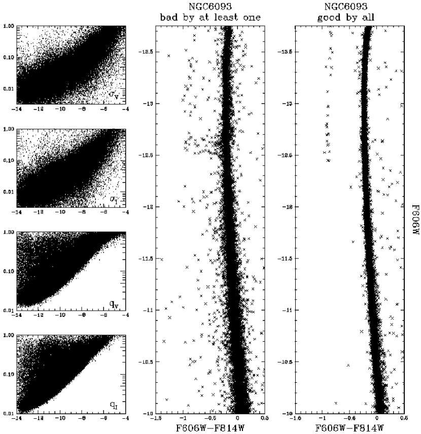
Figure 5: In the left panels, we show from top to bottom $\sigma_{V}$, $\sigma_{I}$, $q_{V}$, and $q_{I}$ as a function of instrumental magnitude for the stars in NGC 6093. The lines delineate the well-measured stars (those below the lines) from those that are less well measured (above the lines). The CMD in the middle panel shows those stars that fell above the line in at least one of the four plots. The CMD on the right shows the stars that appear to be well measured according to all the parameters.

Figure 6 shows the same selection strategy for six different clusters, with a variety of central concentrations. For all the clusters, the quality-selection algorithm from the previous figure is able to identify stars that are not measured well. We note that in crowded centers there is often a tuft of poorly measured stars at around F606W $\sim-12.5$ and F814W $\sim-12.5$ (the diagonal tufts in NGC 6388 and NGC 6441). We have visually inspected these stars in the images and found that these are stars near the crowded centers of clusters with nearby saturated neighbors that have bled into the star’s aperture in one of the filters. Our modeling of the neighbors was not able to simulate such complicated artifacts, therefore a small number of stars suffered unavoidable contamination. Thankfully, these stars can be identified by their large photometric errors.

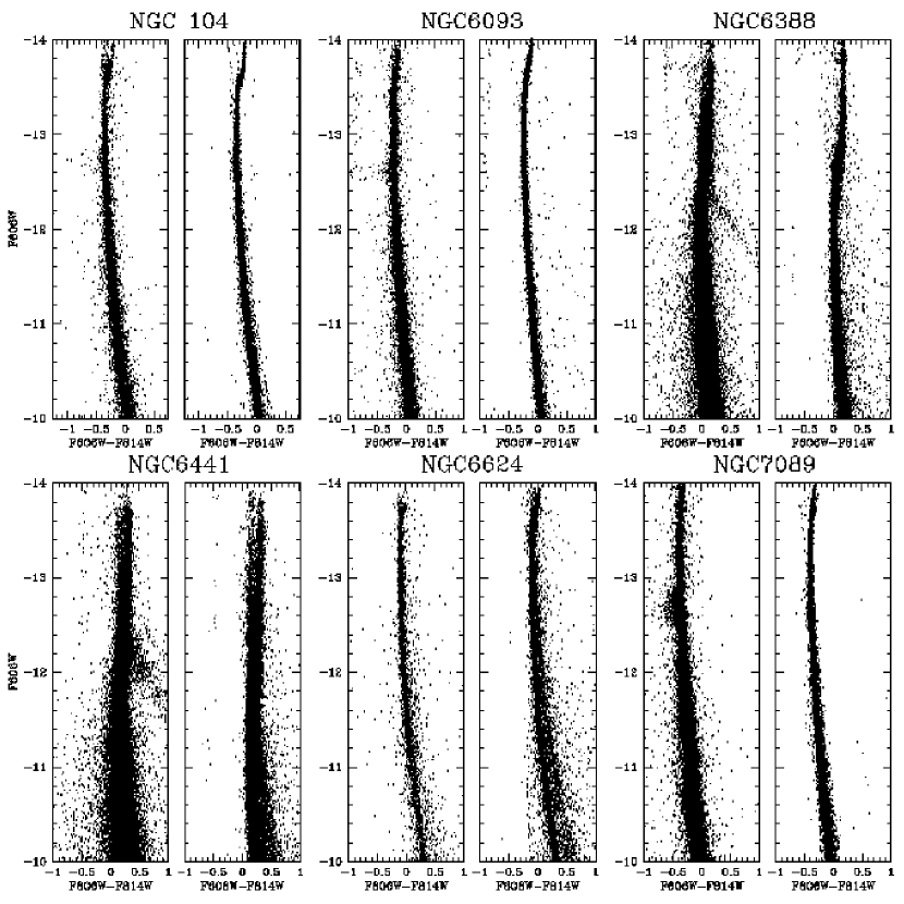
Figure 6: We show the low-quality (left) and high-quality (right) samples for six selected clusters. In NGC 6441 and NGC 6624, we see that the second sequence is not an artifact of the photometry but represents real, well-measured stars—likely a young, foreground population.

Despite these clear improvements in the diagrams, the quality parameters should not be thought of as a panacea. Imposing quality cuts on the data often implicitly imposes other selections as well. For instance, stars that are more isolated are often better measured, so the quality cuts naturally select for stars in the less crowed outskirts of the clusters. If the scientific goal is to study a feature in the CMD that should have no radial dependence (such as the turnoff morphology), then this will not affect the science. But if the goal is to study blue stragglers or binaries, then any radial correlation between these populations and the quality parameters may well produce a biased sample. An examination of the quality parameters as a function of radius could mitigate these selection effects.

7.2 PSF-related errors

The other kind of non-random error that can affect our photometry comes from the PSF itself. Ideally, we would like to measure each star with a large fitting radius or aperture (e.g., $\sim 5$ pixels radius), so that our flux measurement for each star would have as little sensitivity as possible to the details of the PSF model. Unfortunately, almost all of the stars in our fields have neighbors within this radius, and it would be very difficult to disentangle the light from overlapping star images over such a large area. It was obviously necessary to use a smaller fitting region in order to focus on the most relevant pixels for each star. Our standard fitting aperture was 5$\times$5 pixels, corresponding to a radius of $\sim 2.5$ pixels. When there was crowding, we often had to focus even more on the PSF core (see § 5.5). This necessary focus on the central regions of the PSF made us particularly vulnerable to any variations in the PSF that affected what fraction of light fell within the adopted fitting radius.

To understand how PSF variation may have affected our photometry, it is important to consider how the WFC PSF can vary with position or with time. Even if the PSF were perfectly constant over time, it would still have a different shape in different places on the detector due both to distortion and to spatial variations in the chip’s charge-diffusion properties caused by variations in chip thickness (Krist 2005). On account of both of these effects, the fraction of light in the central pixel of the F606W PSF varies from 18% to 22% from location to location on the detector. If this is not accounted for, then fluxes measured by core-fitting can vary by up to 10% (0.1 magnitude). On top of this, spacecraft breathing can introduce an additional 5% variation in the PSF core intensity. To deal with these variations, our PSF model had a temporally constant component that varied with position, and a spatially constant component that accounted for how the PSF in each exposure differed from the library PSF.

Our two-component PSF model did a good job generating an appropriate PSF for each star in each exposure, but the model is not perfect. Unfortunately, when the telescope changes focus, the PSF does not change in exactly the same way everywhere on the detector, and there are residual spatially dependent variations of a few percent in the fraction of light in the core. We considered constructing more elaborate PSF models, but there were simply not enough bright, isolated stars in these fields to allow us to solve for an array of corrections to the library PSF for each exposure. To improve the PSF this way, we would have had to measure the PSF profile out to at least 5 pixels for a large number of stars distributed throughout the field. The centers of most of our clusters were simply too crowded to permit us to model the PSF’s spatial variation empirically. Thus, there is a limit to how well we can know the PSF in each exposure, and this uncertainty naturally impacts our ability to measure accurate fluxes for the stars. It is interesting to note that the same crowding that prevents us from using large apertures when we measure stars also prevents us from measuring much more than the core of the PSF in the centers of clusters. This further limits the accuracy of our measurements.

The main effect that unmodelable PSF variations have on our photometry is to introduce a slight shift in the photometric zero point as a function of the star’s location in the field. On average this shift is zero (thanks to the spatially-constant-adjustment part to the PSF), but the trend with position can be as large as $\pm$0.02 magnitude. These small systematic errors will not be important at all for luminosity-function-type analyses, where stars are counted in wide bins. But the errors can be important for high-precision analyses of the intrinsic width of CMD sequences or for studies of turnoff morphology. In general, the PSF variation affects the F606W and F814W filters differently, so the most obvious manifestation of this systematic error is a slight shift in the color of the cluster sequence as a function of location in the field. This variation, in fact, is very hard to distinguish from a variation in reddening with position, which is certainly present in many of the clusters.

In an effort to examine these color residuals, we first modeled the main-sequence ridge line (MSRL), as in the left panel of Figure 7 by tabulating the observed F606W$-$F814W color as a function of F606W magnitude. We next subtracted from each star’s observed color the MSRL color appropriate for its F606W magnitude. This gave us a vertically straightened sequence (next panel of Fig. 7), with a color residual for each star. In the right array of panels in Figure 7, we examine the location of the observed sequence relative to the MSRL for different places within the field. We see that in some places the cluster sequence systematically lies a little to the red or to the blue of the average MSRL.

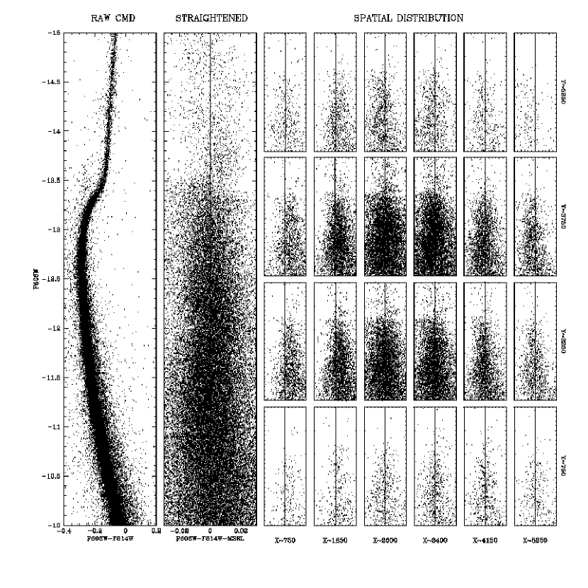
Figure 7: Left: CMD for NGC 5272. Next panel: CMD straightened by MSRL. Right set of panels: the straightened sequence for an array of locations on the detector.

In Figure 8 we plot these color residuals for four clusters as a function of location on the chip. For the first three, we see systematic residuals of $\pm$0.01 magnitude or so. We know that these errors are often related to the PSF because when we have explicitly measured bright stars with larger apertures, the systematic trends were reduced (even though the spread about the MSRL is often greater, because of the stray light that enters a larger aperture). These systematic errors may seem quite small, but from the r.m.s. spread of the independent and artificial-star tests we would expect color errors of less than 0.005 magnitude for each well-exposed star, so the systematic trends do limit how well we can evaluate the intrinsic width of the sequence for each cluster.

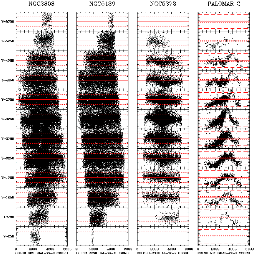
Figure 8: The spatial dependence of the color residuals for four clusters. We divide the 6000$\times$6000 field for each cluster into 12 horizontal slices, each 500 pixels tall in $y$ (the center is marked on the right). Within each panel, we show the color residual from the MSRL as a function of $x$ coordinate. In each of the first three panels the dotted lines represent a color difference of $\pm 0.025$ mag. In the rightmost panel the dashed lines correspond to $\pm 0.25$ mag.

The cluster on the right (Pal 2) exhibits color residuals of $\sim 0.20$ mag, more than ten times those for our typical cluster. These residuals are due to variable reddening for this low-latitude cluster and are largely unrelated to the PSF. Reddening has a similar effect to that of the PSF-related shifts, except that stars affected by reddening should be shifted along the reddening vector, while PSF-related shifts do not necessarily have their $V$ and $I$ shifts correlated.

One way to mitigate the color effect is to introduce an array of empirical corrections across the field and adjust the color for each star according to this table. This procedure does tend to tighten up the CMD and allows us to see more structure (see Milone et al. 2007 for a study of the NGC 1851 CMD), but it is hard to do highly accurate work this way.

8 THE FINAL CATALOG

The procedures described thus far have produced instrumental magnitudes, and positions in an adopted reference frame for each cluster. For our final catalog, however, we need to put the magnitudes onto correct zero points, and give positions in an absolute frame. In addition, improvements are needed in the photometry of the saturated stars, and corrections must be made for the effects of CTE.

8.1 Improving the brightest stars

In designing this project, we chose the length of the short exposures in each cluster in such a way that the horizontal branch would be well exposed but not saturated. Even though the brighter RGB stars were also of interest, it was not efficient to take more than one short exposure for each cluster. The automated finding program discussed in § 5 did find the saturated stars, and it measured a flux for each one by fitting the wings of the PSF to the unsaturated pixels; but such measurements tend to have large errors, both random and systematic.

There is a better way of measuring the saturated stars. Gilliland (2004, G04) has found that when a star saturates in the WFC, its electrons bleed into other pixels, but the total number of electrons due to that star is conserved. If the gain is set to 2, then this information is preserved in the flt image. We were able to verify that the procedure recommended in G04 works for our images, by using it on the stars that are saturated in our long-exposure images, and comparing the resulting fluxes with the accurate fluxes that we had measured for those same stars in our short exposures. The technique that we used was to measure each star in an aperture of 5-pixel radius and include in addition the contiguous saturated pixels that had bled even farther. We found that the fluxes that we measured in this way agreed well with those measured from the unsaturated images in the short exposures. Thus we felt confident in our use of the G04 technique to measure the saturated images in the short exposures, and used these measurements for our final instrumental magnitudes of those stars.

Figure 9 shows a comparison between the CMD obtained from PSF-fitting and the one obtained from the G04 approach. The improvement in the upper parts of the CMD is dramatic, both in the continuity of the sequences and in the photometric spread. Note that towards the bottom of the middle plot the photometric errors increase significantly. This is because the 5-pixel aperture often includes more than just the target star, even for these bright giant-branch stars. PSF-fitting is clearly much better than aperture photometry when stars are not saturated, since most of our accuracy comes from the few central pixels, with their high signal-to-noise ratio. The final photometry uses the better measurement for each star: for stars that are unsaturated in the short exposures, we use the PSF-fit result, but for saturated stars we substitute the aperture-based result.

Figure 9: (Left) The upper part of the CMD for NGC 2808 for stars measured with the wings of the PSF. (Center) The same stars, but with the aperture-based approach. (Right) Combination of the two: PSF-fitting for unsaturated stars, and the aperture-based approach for the saturated stars. Magnitudes are instrumental; saturation sets in at around $-13.75$.

We became aware of the G04 approach only after a large number of the clusters had already been measured. If we had known of it from the beginning, we would have incorporated it directly into our procedures instead of making it a separate post-processing step.

8.2 CTE corrections

The background in many of our short exposures is low enough to raise concerns about the impact of CTE effects on our photometry. The standard corrections for CTE effects are provided for aperture photometry with several aperture sizes, by Riess & Mack (2004, RM04). Since our photometry comes from PSF fitting to the inner 5$\times$5 pixels rather than from aperture photometry, it is unclear which aperture is the most appropriate match to our measurements. In the light of this ambiguity, we proceeded as follows:

We used Eq. 2 of RM04,

$$YCTE=10^{A}\times SKY^{B}\times FLUX^{C}\times{y_{\rm readout}\over{2048}}\times{(MJD-52333)\over{365}},$$

to estimate the CTE correction for each star, given the local sky background, the $y$-position of the star in the flt images, the Modified Julian Date (MJD) of the observation, and the flux of each star as determined from the PSF magnitude. The quantity $y_{\rm readout}$ is the number of $y$ shifts experienced by the pixel; it is simply $y$ for the bottom chip and 2049-$y$ for the top chip.

RM04 provide values of the exponents $A$, $B$, and $C$ for various sizes of the photometric aperture. We chose the values for a 5-pixel aperture, and made those corrections, typically $\sim 0.02$ mag, to our PSF photometry. We then compared the short- and long-exposure photometry for the same stars, after both had been CTE corrected. We then examined the the magnitude differences between the short- and long-exposure photometry, and for almost all clusters the mean difference was zero, with no significant trend as a function of the input parameters $y$-position, sky background, and stellar flux. (See Figure 10 for an example.) In a few cases there was a systematic variation as a function of $y$-position; for these clusters we adopted an aperture size of 7 pixels in the calculation of the CTE corrections, and that eliminated the trend.

Figure 10: The left panel shows the difference between the instrumental magnitudes on the long-exposure frames and the short exposures, for stars in common, as a function of y-position, before the application of the CTE correction for the F606W observations of NGC 6809. The right panel shows the same stars after the CTE correction has been applied.

8.3 Photometric calibration

Thus far we have kept our photometry in instrumental magnitudes, because of their simple relation to counted electrons. (As stated in § 3.1, instrumental magnitudes are simply $-2.5\log N$, where $N$ is the number of counted electrons in the first deep flt image.) We now need to put our magnitudes on a correct zero point.

Unfortunately, our instrumental magnitudes refer to flt images, but the zero point definitions provided by STScI refer to drz images. We therefore measured a few dozen isolated bright stars in the the drz images, using the procedure detailed in Bedin et al.  (2005). We then used the encircled-energy corrections and the zero points given by Sirianni et al.  (2005, S05) to arrive at calibrated VEGAMAG photometry:

$$m_{\rm filter}=-2.5~{}\log_{10}\frac{I_{\rm e^{-}}}{exptime}+Zp^{\rm filter}-\Delta m_{AP_{0.\!\!^{\prime\prime}\!5}-AP_{\infty}}^{\rm filter}-\Delta m_{PSF-AP_{0.\!\!^{\prime\prime}\!5}}^{\rm filter},$$

where “filter” refers to either F606W or F814W. The first term on the right refers to the PSF-fitting photometry in the flt images, the second term is the zeropoint (from S05’s Table 10), and the third term is the correction from the 0$\buildrel\prime\prime\over{.}$5 aperture to the nominally infinite aperture (from S05’s Table 5). The final term must be measured empirically as the difference between our PSF-fitting photometry and the 0$\buildrel\prime\prime\over{.}$5-aperture photometry in the drz image. This is typically close to zero, since our PSFs have been normalized to have unit volume within a radius of 10 flt pixels.

Figure 11 shows the flt$-$drz term (the fourth term) for several clusters for which it was easy to measure. Several of our clusters were so crowded—even in the outskirts—that we could not find enough isolated, unsaturated stars to measure an uncontaminated flux within the 0$\buildrel\prime\prime\over{.}$5 calibration radius. Since the offset appears to be constant (as it should be), we simply adopted the average value over all the clusters ($-0.02$ magnitude). We expect the absolute calibration to be accurate to about 0.01 magnitude for the typical cluster, but because of focus variations that affect the PSF (see § 7.2), the zero-point errors can approach 0.02 magnitude and can vary with position in the field.

Figure 11: The zero-point difference between the PSF-fitting photometry on the flt images and the 0$\buildrel\prime\prime\over{.}$5-aperture on the drz images, determined empirically for several clusters. The error bars indicate the range of stars measured for that cluster, reflecting both random errors and possible systematic errors with position. The dashed line shows the $-0.02$ value adopted as the average. The PSF for the E3 images was observed to be more out of focus than for any other cluster. Also, the E3 field is sparse, which makes it hard to improve the PSF model with an accurate perturbation PSF.

8.4 Absolute astrometric frame

The reference frame we adopted for each cluster was based on the WCS information that the reduction pipeline had placed in the header of the drz image. (See § 3.1.) We expect the absolute astrometric zero point for this frame to be accurate only to 1–2″, since that is what can be expected from errors of the absolute positions of HST’s guide stars (Koekemoer et al.  2005).

To get zero points that were more accurate, we downloaded the 2MASS point-source survey for for the region of each cluster, and found between 40 and 1500 reference stars that we were able to match up with stars in our lists.

We then compared our absolute positions against the absolute positions of the same stars in the 2MASS catalog, and found that the two frames were typically offset by $\sim$1.5″. Figure 12 shows the distribution of offsets for the ensemble of clusters. The typical shift is consistent with the expected astrometric accuracy of HST’s guide-star catalog. Each measured shift came from averaging many tens of stars, each with a typical residual of 0$\buildrel\prime\prime\over{.}$15. Thus our final absolute frame for each cluster should have an absolute accuracy much better than this. (The absolute accuracy of 2MASS positions is given as 15 mas in Skrutskie et al.  2006.) We adjusted the WCS header in each of our stacked images (which will be included with the catalog), to reflect the improved absolute frame.

Figure 12: Offsets between absolute positions constructed from the WCS header of the drz-frame and positions given in the 2MASS catalog. Each point represents one cluster. The dotted circle corresponds to 1″  (20 pixels). Positions in our final catalog have been shifted to agree with the 2MASS zero points.

The relative positions of stars in our field should be much more accurate than their absolute zero point (15 mas corresponds to 0.3 pixel). The non-linear part of the WFC distortion solution is accurate to better than 0.01 pixel (0.5 mas) in a global sense (see Anderson 2005), which is about the random accuracy with which we can measure a bright star in a single exposure. Recently, it has been discovered that the linear terms of the distortion solution have been changing slowly over time (see Anderson 2007). Since our reference frames were based on the drz images (which had not been corrected for this effect), our final frames contain an error of about 0.3 pixel in the off-axis linear terms. Users are therefore cautioned to adopt general 6-parameter linear transformations when relating our frame to other frames. If such transformations are made, our positions should be globally accurate to 0.01 pixel across the field.

8.5 The main catalog

Our entire catalog contains over 6 million stars for 65 clusters, with a median number of 67,000 stars per cluster. Our procedures generated a large amount of information for each star in each cluster, but most users will need only the high-level data for each star. So for each cluster we produced a single file called NGCXXXX.RDVIQ.cal, which has one line for each star found. The columns give reference-frame position, calibrated (i.e., zero-pointed) magnitudes, errors, calibrated RA and Dec, and some general measurement-quality information. The column by column description for this file is given in Table 4.

Table 4: Information in the .RDVIQ.cal file.

Col	Name	Explanation
1	ID	ID number for each star (same as line number)
2	xref	average ref-frame $x$ position
3	yref	average ref-frame $y$ position
4	${\tt V}_{\tt VEGA}$	calibrated F606W magnitude (in the VEGA-mag system)
5	$\sigma_{\tt V}$	RMS error in F606W photometry
6	${\tt VI}_{\tt VEGA}$	calibrated F606W-F814W color
7	$\sigma_{\tt VI}$	RMS error in color
8	${\tt I}_{\tt VEGA}$	calibrated F814W magnitude
9	$\sigma_{\tt I}$	RMS error in F606W photometry
10	${\tt V}_{\tt gnd}$	photometry calibrated to ground-based $V$
11	${\tt I}_{\tt gnd}$	photometry calibrated to ground-based $I$
12	${\tt N}_{\tt V}$	number of $V$ exposures star was found in
13	${\tt N}_{\tt I}$	number of $I$ exposures star was found in
14	wv	source of $F606W$ photometry
		1=unsaturated in deep ; 2=unsaturated in short;
		3=saturated in short ; 4=saturated in deep
15	wi	source of $F814W$ photometry
16	ov	fraction of light in F606W aperture due to neighbors
17	oi	fraction of light in F814W aperture due to neighbors
18	qv	quality of F606W PSF-fit (smaller is better)
19	qi	quality of F814W PSF-fit
20	RA	Right ascension for the star, in degrees
21	Dec	Declination, in degrees

In addition, for each cluster we generated several auxiliary files, which contain the simultaneous-fit fluxes, the exposure-by-exposure photometry, and much more. Finally, we also put together a similar set of files for the artificial-star tests, along with the list of input parameters (x_in, y_in, mv_in, and mi_in). The stacked image in each color will be made available along with the catalog for each cluster.

9 SUMMARY

The ACS Survey of Globular Clusters is the first truly uniform, deep survey of the central regions of a large number of Galactic globular clusters. The observations for each of the 65 clusters were carefully planned in order to provide even spatial coverage of a 3$\times$3-arcminute region near the center of each cluster. To make use of the uniformity of the observations, we developed a reduction strategy that would reduce the data set for each cluster in an automated way, finding as many stars as possible while at the same time minimizing the inclusion of false detections. The stars found were measured as accurately as possible with the best available PSF models.

We adjusted the exposure times for individual clusters in such a way that the final catalog of stars is largely complete down to 0.2 $M_{\odot}$ for the less crowded clusters. We hope that our nearly definitive list of stars will make it easier for future researchers to cross-identify stars in past and future cluster observations.

In addition to the catalog of real stars, we also constructed a standard catalog of artificial-star tests for each cluster that can help assess any incompleteness or photometric biases in the sample. We plan to make this catalog public in the near future with full access to the photometric and astrometric data for each of the 65 clusters via the world-wide web.

Even a cursory glance at the many CMDs in this survey shows that while the clusters all have the same general features, each cluster contains a unique population of stars, representative of its particular star-formation and dynamical history. An early version of this catalog has already led to several papers, including: (1) a study of clusters with no previous HST observations (Sarajedini et al. 2007); (2) the creation of a set of stellar evolutionary tracks matching our photometric system (Dotter  al.  2007); (3) population analysis of the M54/Sgr Color-Magnitude Diagram (Siegel et al. 2007); and (4) discovery of the multiple subgiant branch of NGC 1851 (Milone et al. 2007).

Additional papers are in preparation to study radial profiles, relative ages, cluster mass functions and mass segregation, the Sagittarius clusters, horizontal-branch morphology, the binary populations and their radial gradients, blue stragglers, internal proper motions, and dynamical families of clusters.

References

- (1)
- (2) Anderson, J. & King, I. R. 2006, ACS/ISR 2006-01, PSFs, Photometry, and Astrometry for the ACS/WFC
- (3) Anderson, J. 2007, ACS/ISR 2007-08, Variation of the Distortion Solution of the WFC.
- (4) Armandroff, T. E. 1989, AJ, 97, 375
- (5) Bedin, L. R., Cassisi, S., Castelli, F., Piotto, G., Anderson, J., Salaris, M., Momany, Y., & Pietrinferni, A. 2005, MNRAS, 357, 1038
- (6) Bedin, L. R., Piotto, G., King, I. R., & Anderson, J. 2003, AJ, 126, 247
- (7) Djorgovski, S., & Meylan, G. 1993, Structure and Dynamics of Globular Clusters (eds. S. Djorgovski & G. Meylan), ASPCS, vol. 50 (San Francisco: Astron. Soc. Pacific)
- (8) Djorgovski, S., & King, I. R. 1986, ApJ, 305, L61
- (9) Dotter, A., Chaboyer, B., Jevremovic̀ D., Baron, E., Ferguson, J. W., Sarajedini, A., & Anderson, J. 2007, AJ, 134, 376
- (10) Fruchter, A. S., & Hook, R. N. 2002 PASP 114 792
- (11) Gilliland, R. 2004, ACS/ISR 2004-01, CCD Gains, Full Well Depths, and Linearity up to and Beyond Saturation
- (12) Harris, W. E. 1996, AJ, 112, 1487
- (13) Koekemoer, A. M., McLean, B., McMaster, M., & Jenkner, H. 2005, ACS/ISR 2005-06, Demonstration of a Significant Improvement in the Astrometric Accuracy of HST Data
- (14) Lee, Y. -W., Demarque, P., & Zinn, R. 1994, ApJ, 423, 248
- (15) Milone, A. P., Villanova, S., Bedin, L. R., Piotto, G., Carraro, G., Anderson, J., King, I. R., & Zaggia, S. 2006, A&A, 456, 517
- (16) Milone, A. P., et al. 2007, ApJ, in press
- (17) Piotto. G., et al. 2002, A&A, 391, 945
- (18) Riess, A., & Mack, J. 2004. ACS/ISR 2004-06, Time Dependence of ACS CTE Corrections for Photometry and Future Predictions
- (19) Rosenberg, A., Piotto, G., Saviane, I., & Aparicio, A. 2000a, A&AS, 144, 5
- (20) Rosenberg, A., Aparicio, A., Saviane, I., & Piotto, G. 2000b, A&AS, 145, 451
- (21) Sarajedini, A., et al. 2007, AJ, 133, 1658
- (22) Siegel, M. H., et al. 2007 ApJL 667 57
- (23) Skrutskie, M. F., et al. 2006, AJ, 131, 1163
- (24) Trager, S. C., King, I. R., & Djorgovski, S. 1995, AJ, 109, 218
- (25) Zinn, R. 1980, ApJS, 42, 19
- (26)
- (27)
- (28)