Abstract

We propose a cosmological model which exhibits the phenomenon of self-acceleration: the Universe is attracted to the phase of accelerated expansion at late times even in the absence of the cosmological constant. The self-acceleration is inevitable in the sense that it cannot be neutralized by any negative explicit cosmological constant. The model is formulated in the framework of brane-world theories with a warped extra dimension. The key ingredient of the model is the brane-bulk energy transfer which is carried by bulk vector fields with a $\sigma$-model-like boundary condition on the brane. We explicitly find the 5-dimensional metric corresponding to the late-time de Sitter expansion on the brane; this metric describes an AdS₅ black hole with growing mass. The present value of the Hubble parameter implies the scale of new physics of order 1 TeV, where the proposed model has to be replaced by putative UV-completion. The mechanism leading to the self-acceleration has AdS/CFT interpretation as occurring due to specific dynamics of conformal matter interacting with external “electric” fields. The Universe expansion history predicted by the model is distinguishable from the standard $\Lambda$CDM cosmology.

1 Introduction and summary

One of the open questions of the contemporary physics is the nature of dark energy. The latter term is conventionally used for the unknown substance which is believed to be responsible for the observed acceleration of the cosmological expansion. In the minimal scenario, the dark energy is identified with the cosmological constant (CC). However, the energy scale associated with the value of the CC required to explain the observed dark energy density [1],

$$\rho_{DE}=(0.43\cdot 10^{-10}~{}\mathrm{GeV})^{4}\;,$$ (1)

is much smaller than any other fundamental energy scale existing in particle physics. Thus, one faces the problem of explaining this strong hierarchy [2]. All particle condensates (i.e., those associated with spontaneous symmetry breaking) contribute to CC but have to almost cancel out. Moreover, the CC receives contributions from quantum fluctuations of all fields so that a natural value for it would be

$$\rho^{(\mathrm{natural})}_{\Lambda}\sim\Lambda_{UV}^{4}\;,$$ (2)

where $\Lambda_{UV}$ is the ultra-violet cutoff of the theory. The validity of the Standard Model of particle physics up to energies of order 1 TeV implies that $\Lambda_{UV}\gtrsim 1$ TeV. The latter value of $\Lambda_{UV}$ when substituted into (2) gives the natural value of the CC much larger than the one consistent with observations.

Of course, Eq. (2) is not rigorous: quantum corrections to CC are divergent and can be formally put to any value by renormalization. There exist several proposals to cancel the CC (for reviews see, e.g., Refs. [2, 3, 4]). They can be split in two groups. One group involves proposals based on relaxation mechanisms [5, 6, 7, 8, 9]. These proposals suffer from the “empty Universe” problem (see, e.g., [4]): the relaxation mechanisms drive the Universe to the state practically devoid of matter which is inconsistent with the Hot Big Bang. It is not clear for the moment whether this problem can be consistently resolved without invoking anthropic selection [10]. Another group involves symmetry [11] or quantum gravity [12, 13] arguments. However, these proposals adjust the CC somewhat too well: they predict that the CC is exactly zero. The problem is now reversed: obtaining the Universe undergoing the late-time de Sitter expansion requires fine-tuning.

In this context one would like to construct a setup which excludes the Minkowski space-time from the possible asymptotics of the history of the Universe irrespectively of the value of the CC. Namely, we envisage the following picture. The Universe is driven to the de Sitter phase at late times not by the CC but by some dynamical mechanism. The Hubble parameter of the asymptotic de Sitter space-time may depend on the value of the CC but is always bounded from below by a tiny positive value. This reduces the CC problem to its old form: the need to explain the cancellation of the CC (admittedly, this is the most difficult task) without the risk of being over-precise. An additional requirement one would like to impose on the dynamical mechanism leading to the late-time acceleration of the Universe is that it should not invoke the small energy scale entering Eq. (1) as an input and should not require any particular initial conditions for the evolution of the Universe. It is natural to refer to the scenario described above as “self-accelerated cosmology”.

The model that came closest to the realization of the self-accelerated scenario is the DGP model [14]. It is formulated in flat (4+1)-dimensional space-time with our Universe being represented by a 3-dimensional brane; the key ingredient of the model is the induced gravity term on the brane. Still, the self-accelerated branch of this model suffers from the presence of ghost fields [15, 16], i.e. excitations with negative kinetic term which signal inconsistency of the theory.

In this paper we propose another model which realizes the idea of self-accelerated cosmology. The model is formulated in the context of brane-world scenario with warped extra dimensions [17]. We do not consider the induced gravity term on the brane. Instead, we introduce an energy exchange between the brane and the bulk carried by a triplet of $U(1)$ bulk vector fields [18]. Then, the self-acceleration mechanism can be summarized as follows. As the brane expands, it gives rise to an energy flow from the brane into the bulk. This energy flow, in its turn, results in the formation of a bulk black hole with growing mass. The latter back-reacts on the brane and maintains the brane Hubble parameter constant at late times. Similar ideas were expressed previously in Ref. [20]; our model provides explicit realization of these ideas in the framework of field theory. The brane-bulk energy exchange is kept at the level sufficient to provide the self-accelerated cosmology by a specific Dirichlet boundary condition for the vector fields which forces their squared values on the brane to be equal to a fixed parameter $M^{2}$, see Eq. (5). Note that existence of a continuous energy flux from the brane implies violation of the null energy condition by the brane energy-momentum tensor. This property is dangerous as it can lead to instabilities [21]. Below we briefly discuss this problem and a possible way to resolve it. A more detailed treatment of this issue will be presented elsewhere [22]. In the present paper we concentrate on the cosmological applications of our model.

When the explicit CC on the brane vanishes, the self-accelerated expansion regime at late times corresponds to the value of the would-be CC given by the seesaw formula,

$$\rho_{\Lambda_{eff}}\sim\left(M^{2}/M_{Pl}\right)^{4}\;.$$ (3)

The present dark energy density (1) corresponds to $M$ of order 1 TeV. It is important to stress that self-acceleration mechanism we propose is not equivalent to an implicit introduction of a small positive CC. We check this in two ways. First, we find that in the absence of an explicit CC and matter on the brane the system admits, apart from the self-accelerated solution, also a static solution with Minkowski metric on the brane. However, in contrast to the self-accelerated solution, the Minkowski solution is unstable and is not an attractor of the cosmological evolution. This solves the problem of naturalness of the initial conditions leading to late-time acceleration: in our model the Universe always approaches the de Sitter space at late times. Second, we show that the self-acceleration mechanism cannot be compensated by an explicit introduction of a negative CC on the brane. Namely, depending on the value of the negative CC, the Universe either undergoes the accelerated expansion with essentially the same Hubble parameter corresponding to (3), or collapses. The latter behavior, the collapse for large and negative explicit CC, is similar to the collapse of the Universe in the case of negative CC in the standard Friedman cosmology. Presumably, a (yet unknown) mechanism which cancels the large positive CC, excludes the collapsing cosmological solutions as well, cf. [12, 13].

The self-acceleration mechanism realized in our model has a transparent interpretation in term of the AdS/CFT correspondence [23]. In this language the acceleration is driven by the conformal matter. The cooling of this matter due to the expansion of the Universe is compensated by an energy inflow due to work done by external “electric” fields on the CFT. The latter do not decay rapidly in the expanding Universe in our model. Technically, this is achieved by the specific $\sigma$-model-like conditions on the vector fields, Eq. (5). The CFT interpretation of the self-acceleration mechanism suggests phenomenological generalizations of the model. The cosmological expansion equation in this class of models is distinct from the standard $\Lambda$CDM case, thus providing falsifiable predictions. A careful analysis of this and other phenomenological consequences of our model and its generalizations is left for future work.

The paper is organized as follows. In Sec. 2 we introduce the setup and identify its features that are relevant for cosmology. Section 3 contains qualitative analysis of the cosmological evolution in the model. A more rigorous analysis is performed in Sec. 4 where an explicit solution describing a self-accelerated universe is given. In Sec. 5 we describe the interpretation of this cosmological solution in the spirit of the AdS/CFT correspondence. In Sec. 6 we discuss open issues related to our work. Appendix A presents an explicit example of a brane Lagrangian giving rise to the self-accelerated cosmology. Appendices B and C contain technical details.

2 Setup

We consider a brane-world model based on the setup analogous to that of Ref. [17]. All the fields describing the observable matter are supposed to be localized on a 3-brane. The action of the model is the sum of bulk and brane parts,

$$S=S_{bulk}+S_{brane}\;.$$

The bulk sector consists of gravity described by the standard Einstein–Hilbert action with negative cosmological constant $\Lambda_{5}$ and of a triplet of Abelian bulk vector fields $A_{M}^{a}$, $a=1,2,3$. Thus, for the bulk action we have,

$$S_{bulk}=\int d^{5}x\sqrt{g}\left(-\frac{R}{16\pi G_{5}}-\Lambda_{5}-\frac{1}{4e^{2}}F_{MN}^{a}F^{a\,MN}\right)\;,$$

where

$$F_{MN}^{a}=\partial_{M}A_{N}^{a}-\partial_{N}A_{M}^{a}\;.$$

The brane action is taken in the following form,

$$S_{brane}=\int d^{4}x\sqrt{-\bar{g}}\,\big{(}-\sigma+{\cal L}_{SM}+{\cal L}_{HS}[A_{\mu}^{a},\ldots]\big{)}\;.$$ (4)

Following [17] we impose $Z_{2}$ reflection symmetry across the brane. In the above brane action $\sigma$ is the tension of the brane, ${\cal L}_{SM}$ represents the Standard Model Lagrangian (possibly, including dark matter sector), and ${\cal L}_{HS}$ is a boundary Lagrangian for the vector fields. The dots represent possible dependence of ${\cal L}_{HS}$ on some additional fields localized on the brane. We will refer to the sector described by ${\cal L}_{HS}$ as the “hidden sector”: we assume that there are no direct interactions of the vector fields $A^{a}_{\mu}$ as well as of the other fields entering into ${\cal L}_{HS}$ (except the metric $g_{\mu\nu}$) with the Standard Model fields.

For the brane tension we write

$$\sigma=\sqrt{-3\Lambda_{5}/4\pi G_{5}}+\rho_{\Lambda}\;.$$

As we will see shortly $\rho_{\Lambda}$ plays the role of the 4-dimensional CC. We assume that there is some mechanism ensuring that $\rho_{\Lambda}$ is much smaller than its natural value (2). Without knowledge of the details of this mechanism we cannot be more concrete and say what value of $\rho_{\Lambda}$ it predicts. A reasonable possibility is that $\rho_{\Lambda}$ is set equal to zero but other options cannot be excluded. So we will keep $\rho_{\Lambda}$ explicitly in the formulas in order to be able to control its effect on the cosmological evolution.

The precise form of the hidden sector Lagrangian is not important for our purposes. For the study of cosmology it is sufficient to require the following properties:

(1) Variation of ${\cal L}_{HS}$ gives the following boundary condition for the vector fields on the brane:

$$\bar{g}^{\mu\nu}A^{a}_{\mu}A^{b}_{\nu}\Big{|}_{brane}=-M^{2}\delta^{ab}\;,$$ (5)

where $\bar{g}^{\mu\nu}$ is the induced metric on the brane, and $M$ is some parameter of dimension of mass. Though the condition (5) has a generally covariant form it can be satisfied only if the vector fields are non-zero so that the local Lorentz symmetry is spontaneously broken. Note also that Eq. (5) explicitly breaks the $U(1)$ gauge symmetries of the bulk action. Having in mind an analogy with $\sigma$-models of particle physics one expects that the use of the condition (5) is justified at energies below $M$ which are relevant for late-time cosmology. On the other hand, at energies above $M$ some UV-completion of the theory is required.

(2) The energy density of the hidden sector matter dilutes, $\rho_{HS}\to 0$, as the brane undergoes the cosmological expansion. In other words, we assume that the hidden sector as well as the Standard Model sector does not contain any CC. In order not to contradict the observational data $\rho_{HS}$ should dilute at the same rate or faster than the energy density of dust.

An explicit example of the Lagrangian ${\cal L}_{HS}$ satisfying the requirements (1), (2) is presented in appendix A.

We make the following assumptions about the order-of-magnitude values of the parameters of our setup. The bulk physics is governed by the energy scale of order or slightly below the Planck mass. Thus, we have

$$G_{5}\sim M_{Pl}^{-3}~{},~{}~{}~{}e^{2}\sim M_{Pl}^{-1}~{},~{}~{}~{}\Lambda_{5}\sim M_{Pl}^{5}\;.$$ (6)

On the other hand, the scale $M$ entering into Eq. (5) is assumed to be much smaller than the Planck mass. Below we will take $M\sim\text{1 TeV}$ in order to fit the observed acceleration rate of the Universe.

3 Cosmology: qualitative discussion

3.1 Cosmological Ansatz

We now turn to the discussion of cosmology in the model described above. The general Ansatz for the metric and vector fields, invariant under 3-dimensional translation and rotations, has the form

$$ds^{2}=F(t,\zeta)(dt^{2}-d\zeta^{2})-r^{2}(t,\zeta){(dx^{i})}^{2};$$ (7)

$$A^{a}_{i}=MA(t,\zeta)\,\delta^{a}_{i}~{},~{}~{}~{}~{}~{}A^{a}_{t}=A^{a}_{\zeta}=0.$$ (8)

Equations (8) imply that the vector fields $A^{a}_{M}$ form an orthogonal spacelike triad; such a configuration is invariant under 3-dimensional rotations supplemented by simultaneous rotations in the internal space. Embedding of the brane into the space with metric (7) is described by a set of functions $x^{M}(y^{\mu})$. Choosing $x^{i}=y^{i}$ one is left with two functions, $t_{B}(\tau)$ and $\zeta_{B}(\tau)$, describing the trajectory of the brane on the $(t,\zeta)$ plane. Here $\tau$ is a time parameter on the brane, see Fig. 1.

Figure 1: The coordinate frame used in the text. Thick curve shows the trajectory of the brane. The space-time considered in the text consists of two copies of white region (above the thick curve) glued across the brane trajectory and related by $Z_{2}$ symmetry. Gray region is cut off.

It is convenient to choose $\tau$ to be the cosmological time. Then the induced metric on the brane takes the Robertson–Walker form

$$d\bar{s}^{2}=d\tau^{2}-a^{2}(\tau)(dx^{i})^{2}\;.$$ (9)

Here $a(\tau)=r(t_{B}(\tau),\zeta_{B}(\tau))$, and the functions $t_{B}$, $\zeta_{B}$ obey the condition

$$F(t_{B},\zeta_{B})\big{(}\dot{t}_{B}^{2}-\dot{\zeta}_{B}^{2}\big{)}=1\;,$$

where dot denotes derivative with respect to $\tau$. The motion of the brane is affected by the bulk metric via the junction conditions. Imposing $Z_{2}$ reflection symmetry across the brane one obtains,

$$4\pi G_{5}T_{(br)\,\tau}^{\tau}=-3\left(\frac{\partial_{t}r}{r}\dot{\zeta}_{B}+\frac{\partial_{\zeta}r}{r}\dot{t}_{B}\right)\;,$$ (10a)

$$4\pi G_{5}T_{(br)\,i}^{j}=-\left[\left(\frac{2\partial_{t}r}{r}+\frac{\partial_{t}F}{2F}\right)\dot{\zeta}_{B}+\left(\frac{2\partial_{\zeta}r}{r}+\frac{\partial_{\zeta}F}{2F}\right)\dot{t}_{B}+\frac{1}{\sqrt{F}\dot{t}_{B}}\frac{d}{d\tau}(\sqrt{F}\dot{\zeta}_{B})\right]\delta_{i}^{j}\;.$$ (10b)

Finally, the boundary conditions (5) relate the boundary value of the function $A(t,\zeta)$ to the scale factor of the brane metric,

$$A(t_{B}(\tau),\zeta_{B}(\tau))=a(\tau)\;.$$ (11)

This equation implies that the cosmological expansion of the brane acts as a source for the bulk vector fields. As we will see, this lies at the origin of the self-acceleration mechanism in our model.

The junction conditions (10) are simplified if the Hubble parameter $H\equiv\dot{a}/a$ on the brane is small compared to the curvature of the bulk. In this case one expects the distortion of the bulk due to the vector fields emitted by the brane to be small near the brane. Then the metric in the vicinity of the brane is approximately that of AdS₅:

$$F=\frac{1+2\phi(t,\zeta)}{(k\zeta)^{2}}~{},~{}~{}~{}~{}r=\frac{1+\psi(t,\zeta)}{k\zeta}\;,$$ (12)

where $k\equiv\sqrt{-4\pi G_{5}\Lambda_{5}/3}$ is the inverse AdS radius, and $\phi,\psi\ll 1$. Expanding Eqs. (10) to the linear order in $\phi,\psi$ and to quadratic order in $H/k$ one finds the equations governing the cosmological expansion of the brane,

$$H^{2}=\frac{8\pi G_{N}}{3}(\rho_{\Lambda}+\rho)+2k^{2}(\phi+\zeta\partial_{\zeta}\psi)\big{|}_{brane}\;,$$ (13)

$$\dot{H}=-4\pi G_{N}(\rho+p)+k^{2}(\zeta\partial_{\zeta}\phi-\zeta\partial_{\zeta}\psi)\big{|}_{brane}\;.$$ (14)

Here $G_{N}=G_{5}k$ is the four-dimensional Newton constant, and $\rho$, $p$ are the energy density and pressure of the brane matter (including both the Standard Model and hidden sector fields). Without the terms on the r.h.s. containing the functions $\phi$, $\psi$, equations (13), (14) would describe the standard cosmology with the cosmological constant $\rho_{\Lambda}$. The above terms are responsible for the modification of the brane cosmology in our model; they are to be found from the bulk dynamics.

Let us comment on the validity of the approximation (12). We will check below that it is indeed valid in the vicinity of the brane if

$$H/k\ll 1\;.$$

The latter inequality is readily satisfied in the regime of interest: eventually we want $H$ to be comparable to the present Hubble parameter of the Universe, while $k$ is assumed to be of order $M_{Pl}$. On the other hand the form (12) is inapplicable far from the brane: we will see shortly that the effect of the vector fields on the space-time geometry increases deep into the bulk and leads to strong deviation of the metric from that of AdS₅.

3.2 Vector fields in external metric

Let us analyze the behavior of the vector fields in the curved metric (7). Using the cosmological Ansatz (8) one derives their equation of motion

$$\partial_{t}(r\partial_{t}A)-\partial_{\zeta}(r\partial_{\zeta}A)=0$$ (15)

and the expressions for the components of their energy–momentum tensor:

$$T_{tt}=T_{\zeta\zeta}=\frac{3M^{2}}{2e^{2}r^{2}}\big{(}(\partial_{t}A)^{2}+(\partial_{\zeta}A)^{2}\big{)}\;,$$ (16a)

$$T_{t\zeta}=\frac{3M^{2}}{e^{2}r^{2}}\partial_{t}A\partial_{\zeta}A\;,$$ (16b)

$$T_{ij}=\delta_{ij}\frac{M^{2}}{2e^{2}F}\big{(}(\partial_{t}A)^{2}-(\partial_{\zeta}A)^{2}\big{)}\;.$$ (16c)

Note that non-vanishing value of $T_{t\zeta}$ implies non-vanishing energy flux along the $\zeta$-direction carried by the vector fields.

It is instructive to neglect for the moment the backreation of the vector fields on the metric and consider their evolution in the external AdS₅ geometry. Accordingly, one sets

$$F=\frac{1}{(k\zeta)^{2}}~{},~{}~{}~{}r=\frac{1}{k\zeta}\;.$$ (17)

Let us also forget about the brane for a while and consider the Dirichlet boundary condition for the vector field at the AdS boundary,

$$A(t,\zeta)\to A^{(0)}(t)~{},~{}~{}~{}\zeta\to 0^{+}\;.$$ (18)

The relevance of this problem for the original cosmological setup will become clear shortly. Performing the Fourier decomposition,

$$A(t,\zeta)=\int\frac{d\omega}{2\pi}\tilde{A}(\omega,\zeta){\rm e}^{-i\omega t}\;,$$

and solving Eq. (15) one finds

$$\tilde{A}(\omega,\zeta)=\frac{i\pi}{2}\omega\zeta H_{1}^{(1)}(\omega\zeta)\tilde{A}^{(0)}(\omega)\;.$$ (19)

This expression suggests two important observations.

First, the vector fields are almost constant at distances $\zeta\ll 1/\omega$ from the AdS boundary,

$$\frac{\tilde{A}(\omega,\zeta)-\tilde{A}(\omega,0)}{\tilde{A}(\omega,0)}\ll 1~{},~{}~{}~{}\text{for}~{}~{}\omega\zeta\ll 1\;.$$

The latter condition is satisfied by the position $\zeta_{B}$ of the brane in our cosmological setup. Indeed, the characteristic frequency entering the problem can be estimated as

$$\omega\sim\frac{1}{A(t_{B},\zeta_{B})}\frac{dA(t_{B},\zeta_{B})}{dt_{B}}\;.$$ (20)

Using the relation (11) between the boundary value of the vector field and the scale factor on the brane one obtains,

$$\omega\zeta_{B}\sim\frac{\zeta_{B}}{a}\frac{da}{dt_{B}}=\zeta_{B}\frac{da}{d\tau}=\frac{H}{k}\ll 1\;,$$ (21)

where in the last equality we substituted $a=1/(k\zeta_{B})$. Therefore one can simplify the set of equations determining the cosmological solution by replacing Eq. (11) with

$$A(t_{B}(\tau),0)=a(\tau)\;.$$ (22)

Instead of being formulated on the moving brane, the boundary condition for the vector field is now imposed on the fixed timelike surface — the AdS boundary.

Second, the formula (19) can be used to estimate the backreaction of the vector fields on the metric. For example, let us consider the trace of energy–momentum tensor of these fields. From Eqs. (16) one obtains that the contribution of a given harmonic at $\omega\zeta\gg 1$ has the form

$$T_{M}^{M}=-\frac{3\pi M^{2}k\omega|\tilde{A}^{(0)}(\omega)|^{2}}{64e^{2}}(k\zeta)^{3}\;.$$

We see that $T_{M}^{M}$ grows into the bulk. Thus, at large distance from the AdS boundary the backreaction of the vector fields on the space–time geometry gets large and should be properly taken into account. We proceed to this task.

3.3 Account for backreaction

The above analysis suggests the following physical picture. The cosmological expansion of the brane generates the bulk vector fields. The $T_{t\zeta}$ component of the energy–momentum tensor of these fields is non-zero, so they carry a flux of energy out of the brane. Due to the warping of the bulk metric the energy density of the flux grows into the bulk leading to formation of a black hole. It is known [19] that the presence of a constant mass black hole in the bulk affects the cosmology on the brane via the so called “dark radiation” term which dilutes as $1/a^{4}$ at late times. In our case the mass of the black hole is not constant: it grows with time due to the continuous inflow of energy from the brane. This leads to nontrivial consequences at late times.

To determine the growth rate of the black hole mass rigorously, one needs to solve the system consisting of equations of motion for the vector fields and the bulk Einstein equations. This will be done in the next section for the case of the self-accelerated cosmological Ansatz. For the moment we adopt a simplified strategy which allows to catch the qualitative features of the resulting cosmology. Namely, we will solve for the vector fields in the background of a static black hole. The energy flux given by this solution will be then inserted into the energy conservation equation in order to calculate the dependence of the black hole mass on time. Finally, we will use the metric of the black hole with time dependent mass to evaluate the bulk terms in the effective Friedman equation (13) on the brane.

A bulk black hole with mass ${\cal M}$ is described by the AdS–Schwarzschild metric,

$$ds^{2}=F(r)dt^{2}-\frac{dr^{2}}{k^{2}F(r)}-r^{2}dx_{i}^{2}\;,$$ (23)

where

$$F(r)=r^{2}-\frac{r_{h}^{4}}{r^{2}}\;,$$ (24)

and the Schwarzschild radius $r_{h}$ is related to the black hole mass ${\cal M}$ as follows,

$$r_{h}=\left(\frac{8G_{5}k^{2}{\cal M}}{3\pi}\right)^{1/4}\;.$$ (25)

This metric can be cast into the form (7) with $\zeta$ determined by the differential equation

$$\frac{d\zeta}{dr}=-\frac{1}{kF}\;.$$

Explicitly,

$$\zeta=-\frac{1}{4kr_{h}}\mathop{\rm ln}\nolimits\left[\frac{r-r_{h}}{r+r_{h}}\right]-\frac{1}{2kr_{h}}\left[\mathop{\rm arctg}\nolimits{\frac{r}{r_{h}}}-\frac{\pi}{2}\right]\;.$$ (26)

In this background the vector equation (15) takes the form

$$-\partial_{\zeta}^{2}A-\frac{d\mathop{\rm ln}\nolimits r}{d\zeta}\partial_{\zeta}A+\partial_{t}^{2}A=0\;.$$ (27)

To understand the structure of the solutions to this equation let us solve it with the Dirichlet condition on the AdS boundary,

$$A(t,\zeta=0)=A_{\omega}^{(0)}{\rm e}^{-i\omega t}\;.$$ (28)

One looks for the solution in the form $A=A_{\omega}(\zeta){\rm e}^{-i\omega t}$. Let us consider the case of small frequencies,

$$\omega\ll kr_{h}\;.$$ (29)

Then, the solution can be constructed in the following way: one solves Eq. (27) in two regions, $\zeta\ll 1/\omega$ and $\zeta\gg 1/kr_{h}$, and matches the solutions in the intersection of these regions, $1/kr_{h}\ll\zeta\ll 1/\omega$. At small values of $\zeta$ the function $A_{\omega}(\zeta)$ varies slowly with $\zeta$ and one can approximate its time derivatives by their values on the AdS boundary,

$$\partial_{t}^{2}A_{\omega}\approx-\omega^{2}A_{\omega}^{(0)}\;.$$ (30)

Equation (27) yields

$$\partial_{\zeta}A_{\omega}=-\frac{\omega^{2}A^{(0)}_{\omega}}{4kr}\left(-\mathop{\rm ln}\nolimits\left[\frac{r^{4}}{r^{4}_{h}}-1\right]+C_{\omega}\right)\;,$$ (31)

where $C_{\omega}$ is the integration constant. The range of validity of this formula is restricted by the condition (30) which translates into

$$\zeta\ll\frac{1}{\omega}~{},~{}\frac{1}{\omega\sqrt{C_{\omega}}}\;.$$ (32)

In the region $\zeta\gg 1/kr_{h}$ the expression (31) takes the form,

$$\partial_{\zeta}A_{\omega}=-\frac{\omega^{2}A_{\omega}^{(0)}}{4kr_{h}}\left(-3\mathop{\rm ln}\nolimits 2-\frac{\pi}{2}+C_{\omega}\right)-\omega^{2}A_{\omega}^{(0)}\zeta\;.$$ (33)

On the other hand, at $\zeta\gg 1/kr_{h}$ the radial function $r(\zeta)$ gets stabilized at the value of the Schwarzschild radius, and the second term in Eq. (27) vanishes. So, in this region the solutions of Eq. (27) are free waves. We take the outgoing solution

$$A_{\omega}(\zeta)=A_{\omega}^{(1)}{\rm e}^{i\omega\zeta}\;.$$

At $\zeta\ll 1/\omega$ this formula gives

$$\partial_{\zeta}A_{\omega}=i\omega A^{(1)}_{\omega}-\omega^{2}A^{(1)}_{\omega}\zeta\;.$$

Comparing this expression with Eq. (33), one obtains

$$A_{\omega}^{(0)}=A_{\omega}^{(1)}\;,$$ (34a)

$$C_{\omega}=-i\frac{4kr_{h}}{\omega}+3\mathop{\rm ln}\nolimits 2+\frac{\pi}{2}\approx-i\frac{4kr_{h}}{\omega}\;.$$ (34b)

Note, that though $C_{\omega}$ is large, $|C_{\omega}|\gg 1$, the second inequality in (32) is still compatible with $\zeta\gg 1/kr_{h}$. Substitution of (34b) into Eq. (31) yields at $\zeta\ll 1/\omega$,

$$\partial_{\zeta}A_{\omega}=\frac{\omega^{2}A^{(0)}_{\omega}}{4kr}\mathop{\rm ln}\nolimits\left[\frac{r^{4}}{r^{4}_{h}}-1\right]+\frac{i\omega r_{h}}{r}A^{(0)}_{\omega}\;.$$ (35)

Due to the condition (29) the first term on the r.h.s. of Eq. (35) is small in comparison with the second one if the logarithm is not too large. We will see below that this condition is satisfied by the solution we are interested in.

It is straightforward to generalize the formula (35) to the case of an arbitrary dependence of the Dirichlet boundary condition on time,

$$A(t,\zeta=0)=A^{(0)}(t)\;.$$

Omitting the first term on the r.h.s in Eq. (35) one obtains

$$\partial_{\zeta}A=-\frac{r_{h}}{r}\partial_{t}A^{(0)}\;.$$ (36)

This expression is valid when the characteristic frequency $\omega\sim\partial_{t}A^{(0)}/A^{(0)}$ satisfies the inequality (29).

The next step is to determine the change of the metric due to the inflow of energy from the brane into the black hole. The increase of the black hole mass is given by the formula

$$\partial_{t}{\cal M}=\frac{2\pi^{2}}{k^{3}}\sqrt{g}\,T^{\zeta}_{t}\;.$$

It is convenient to evaluate the r.h.s. of this equation on the brane. Using Eqs. (16b), (22) and (36) one obtains

$$\partial_{t}{\cal M}=\frac{6\pi^{2}M^{2}}{k^{3}e^{2}}r_{h}(\partial_{t}a)^{2}\;.$$

Substitution of the relation (25) yields the following time-dependence of the Schwarzschild radius,

$$r_{h}=\left(\frac{3\lambda}{2k}\int dt\,(\partial_{t}a)^{2}\right)^{1/3}\;,$$ (37)

where we introduced

$$\lambda=\frac{8\pi G_{5}M^{2}}{e^{2}}\;.$$ (38)

Note that with our assumptions about the hierarchy among the model parameters discussed in Sec. 2, we have $\lambda\sim(M/M_{Pl})^{2}\ll 1$.

One proceeds by extracting the functions $\phi$ and $\psi$ defined in Eq. (12) from the metric (23) and by substituting them into the effective Friedman equation (13). One obtains,

$$H^{2}=\frac{8\pi G_{N}}{3}(\rho_{\Lambda}+\rho)+\frac{k^{2}r_{h}^{4}}{a^{4}}\;,$$

where we made use of the relation $a=1/(k\zeta_{B})$. Finally, Eq. (37) gives,

$$H^{2}=\frac{8\pi G_{N}}{3}(\rho_{\Lambda}+\rho)+\delta\;,$$ (39a)

where

$$\delta=\frac{k^{2}}{a^{4}}\left(\frac{3\lambda}{2k}\int d\tau\,a\dot{a}^{2}\right)^{4/3}\;.$$ (39b)

In the last formula we changed the integration variable from the conformal time $t$ to the proper time $\tau$ on the brane using $d\tau=adt$.

Let us discuss our result. Equations (39) describe the cosmological evolution in terms of brane variables alone. The contribution of the bulk is encoded in the term (39b) which is nonlocal in time. This feature of our setup makes it different from other models of dark energy. In particular, the expansion history of the Universe at the epoch of transition from matter to dark energy domination is expected to be distinguishable from the standard $\Lambda$CDM case.

The non-locality of Eq. (39a) somewhat complicates its exact solution. However, the qualitative effect of (39b) is easy to work out. Let us first consider the case when $\delta$ is small and the cosmological evolution is dominated by matter with equation of state $p=w\rho$, $w<1$. Then one has,

$$\rho\propto a^{-3(1+w)}\;,$$

and

$$a\propto\tau^{\frac{2}{3(1+w)}}\;.$$

Substituting this expression into Eq. (39b) one notices that the integral is saturated at the upper limit. This implies that the choice of the integration constant is irrelevant at the late stages of the cosmological evolution. One obtains,

$$\delta=\left(\frac{2\lambda}{3(1-w^{2})k}\right)^{4/3}\frac{k^{2}}{\tau^{4/3}}=\left(\frac{\lambda^{2}k}{(1-w)^{2}H}\right)^{2/3}H^{2}\;.$$

We see that the $\delta$ term dilutes slowlier than the contribution of the ordinary matter,

$$\delta\propto a^{-2(1+w)}\;.$$

Thus eventually it starts to dominate the cosmological expansion. To figure out what happens in this case we consider the opposite limit of small ordinary matter density, $\frac{8\pi G_{N}}{3}\rho\ll~{}H^{2}$. The solution to Eq. (39a) is approximately given by exponential expansion, $a\propto{\rm e}^{H\tau}$ and the Friedman equation takes the form,

$$H^{2}=\frac{8\pi G_{N}}{3}(\rho_{\Lambda}+\rho)+\left(\frac{\lambda^{2}k}{4H}\right)^{2/3}H^{2}\;.$$ (40)

One concludes that as the matter on the brane dilutes the cosmological expansion is attracted to the self–accelerated fixed point.

The asymptotic Hubble parameter depends on the explicit cosmological constant $\rho_{\Lambda}$, see Fig. 2.

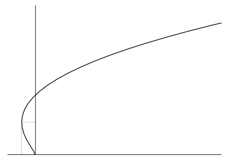
Figure 2: Dependence of the asymptotic Hubble parameter on the explicit cosmological constant $\rho_{\Lambda}$. Only the solutions from the branch $BC$ are stable and can be reached in the course of the cosmological evolution.

For the case $\rho_{\Lambda}=0$ it takes the value

$$H_{c}=\lambda^{2}k/4\;.$$

Recalling the assumptions (6) about the parameters of the model one observes that $H_{c}$ corresponds to the effective energy density given by the seesaw formula (3). The present value of the Hubble parameter is obtained if $M\sim\text{1 TeV}$.

We stress that the self-acceleration mechanism described above is not equivalent to an implicit introduction of the CC. Indeed, for $\rho_{\Lambda}=\rho=0$ equations (39) admit, apart from the exponentially expanding solution, a static solution with $H=0$. However, inspection of Eqs. (39) shows that this solution is unstable: addition of a small amount of matter drives it to the self-accelerating regime. Moreover, one cannot neutralize self-acceleration by introducing a negative $\rho_{\Lambda}$. Let us discuss this issue in more detail. If the matter density $\rho$ is zero and the cosmological constant is negative but not too large,

$$0\geq\rho_{\Lambda}\geq\rho_{min}\equiv-\frac{H_{c}^{2}}{18\pi G_{N}}\;,$$

equations (39) have two branches of solutions, see Fig. 2. However, one can show that the solutions of the branch $AB$ are unstable: they are destroyed by the introduction of matter. Thus, only the solutions of the branch $BC$ can be reached in the course of the cosmological evolution. The Hubble parameter on this branch is bounded from below by $H_{min}=(2/3)^{3/2}H_{c}$. If $\rho_{\Lambda}<\rho_{min}$ there are no solutions to Eqs. (39) unless there is some matter on the brane, $\rho\neq 0$. We solved Eqs. (39) numerically in the case of nonrelativistic matter and $\rho_{\Lambda}<\rho_{min}$ and found that the Universe eventually collapses. Thus, the fate of the Universe is restricted to two possibilities, depending on the value of $\rho_{\Lambda}$: the Universe either undergoes a de Sitter phase with the Hubble parameter greater than $H_{min}$ or collapses. In other words, if the Universe is not collapsing it is inevitably self-accelerating.

Let us check various approximations we made in deriving Eqs. (39). Using Eq. (37) we observe that the condition (29) is satisfied if

$$H\ll\sqrt{\lambda}k\;.$$ (41)

For our choice of parameters $\sqrt{\lambda}k\sim M$ and the requirement (41) is indeed satisfied for most stages of the cosmological evolution. A problem arises with the quasistationary approximation for the bulk metric. Indeed, from Eq. (37) one concludes that $\partial_{t}r_{h}/r_{h}\sim\partial_{t}a/a$ and therefore the metric evolves at the same rate as the vector fields. A priori, this means that the formulas of this section should be taken with a grain of salt and are valid only qualitatively. However, we expect the final result, Eqs. (39) to be correct. This is supported by the explicit solution of the time-dependent Einstein equations for the case of self-accelerated cosmology in Sec. 4 and the interpretation in terms of AdS/CFT correspondence in Sec. 5.

4 Self-accelerated solution

In this section we explicitly solve the system of bulk equations for the metric (7) with Ansatz (8) for the vector fields and show that the model possesses a self-accelerated solution. It is convenient to write the equations of motion in the light–cone coordinates

$$u=k(t-\zeta)~{},~{}~{}~{}v=k(t+\zeta)\;.$$ (42)

A straightforward calculation yields the Einstein equations,

$$-\frac{\partial_{v}^{2}r}{r}+\frac{\partial_{v}F\partial_{v}r}{Fr} =\frac{\lambda}{r^{2}}(\partial_{v}A)^{2}\;,$$ (43a)

$$-\frac{\partial_{u}^{2}r}{r}+\frac{\partial_{u}F\partial_{u}r}{Fr} =\frac{\lambda}{r^{2}}(\partial_{u}A)^{2}\;,$$ (43b)

$$-\partial_{u}\partial_{v}\mathop{\rm ln}\nolimits{F}-\frac{\partial_{u}\partial_{v}r}{r}+\frac{4\partial_{u}r\partial_{v}r}{r^{2}} =\frac{\lambda}{r^{2}}\partial_{u}A\partial_{v}A\;,$$ (43c)

$$\frac{\partial_{u}\partial_{v}r}{r}+\frac{2\partial_{u}r\partial_{v}r}{r^{2}} =-F\;.$$ (43d)

The equation for the vector fields takes the form

$$\partial_{u}(r\partial_{v}A)+\partial_{v}(r\partial_{u}A)=0\;.$$ (44)

One notices that the system (43), (44) is invariant under dilatations,

$$A(u,v)\mapsto\gamma A(\gamma u,\gamma v)\;,~{}~{}~{}r(u,v)\mapsto\gamma r(\gamma u,\gamma v)\;,~{}~{}~{}F(u,v)\mapsto\gamma^{2}F(\gamma u,\gamma v)\;,$$ (45)

where $\gamma$ is an arbitrary constant. In general, this symmetry is broken by embedding of the brane and by the boundary condition (11).

An exception from this rule, which is of primary interest to us, is the case of inflating brane. As discussed in Sec. 3.1 the metric in the vicinity of the brane is close to the metric of AdS₅, see Eqs. (12). The inflating brane is embedded into the AdS space along the straight line

$$\zeta=-\frac{H}{k}t~{},~{}~{}~{}t<0\;,$$

where we used the relation $H\ll k$. Obviously, this embedding respects the symmetry (45). Due to the form of the scale factor,

$$a=-\frac{1}{Ht}\;,$$ (46)

the boundary condition (11) is also invariant under the transformations (45).

The general Ansatz invariant under the symmetry (45) has the form

$$A=-\frac{1}{\sqrt{\lambda}u}\alpha\left(\frac{v}{u}\right)~{},~{}~{}~{}r=-\frac{1}{u}\beta\left(\frac{v}{u}\right)~{},~{}~{}~{}F=\frac{1}{u^{2}}f\left(\frac{v}{u}\right)\;.$$ (47)

Its substitution into Eqs. (43), (44) reduces these equations to a system of ordinary differential equations for the functions $\alpha$, $\beta$, $f$ depending on a single variable $x=v/u$. One obtains,

$$-\frac{\beta^{\prime\prime}}{\beta}+\frac{f^{\prime}\beta^{\prime}}{f\beta} =\left(\frac{\alpha^{\prime}}{\beta}\right)^{2}\;,$$ (48a)

$$-\frac{\beta^{\prime\prime}}{\beta}-\frac{2\beta^{\prime}}{x\beta}+\frac{f^{\prime}\beta^{\prime}}{f\beta}+\frac{f^{\prime}}{xf} =\left(\frac{\alpha^{\prime}}{\beta}+\frac{\alpha}{x\beta}\right)^{2}\;,$$ (48b)

$$\left(\frac{f^{\prime}}{f}\right)^{\prime}+\frac{\beta^{\prime\prime}}{\beta}+\frac{f^{\prime}}{xf}-\frac{2\beta^{\prime}}{x\beta}-4\left(\frac{\beta^{\prime}}{\beta}\right)^{2} =-\left(\frac{\alpha^{\prime}}{\beta}\right)^{2}-\frac{\alpha\alpha^{\prime}}{x\beta^{2}}\;,$$ (48c)

$$\frac{\beta^{\prime\prime}}{\beta}+\frac{4\beta^{\prime}}{x\beta}+2\left(\frac{\beta^{\prime}}{\beta}\right)^{2} =\frac{f}{x}\;,$$ (48d)

$$\frac{\alpha^{\prime\prime}}{\alpha}+\frac{\beta^{\prime}\alpha^{\prime}}{\beta\alpha}+\frac{5\alpha^{\prime}}{2x\alpha}+\frac{\beta^{\prime}}{2x\beta} =0\;.$$ (48e)

The first four equations correspond to the Einstein equations, while the last one is the equation of motion of the vector fields; only three equations out of five are independent. One looks for a solution to these equations in the interval $0<x<1$. The end-points $x=0$ and $x=1$ of this interval map to the horizon $\zeta=-t$ and the AdS boundary $\zeta=0$, respectively. Note that we again used the inequality $H\ll k$ and identified the brane with the AdS boundary. We require that the solution should be regular at the horizon: the functions $\alpha$, $\beta$, $f$ must be continuous at $x=0$. The value of the function $\alpha$ at the AdS boundary is fixed by Eqs. (22), (46), (47):

$$\alpha\to\alpha_{0}\equiv\frac{\sqrt{\lambda}k}{H}~{},~{}~{}~{}~{}~{}x\to 1\;.$$ (49)

The behavior of the functions $\beta$, $f$ near the boundary is determined from the requirement that the metric in this region approximates that of AdS₅. Comparing Eqs. (17) with (47) one obtains,

$$\beta\to\frac{2}{1-x}~{},~{}~{}~{}f\to\frac{4}{(1-x)^{2}}~{},~{}~{}~{}~{}x\to 1\;.$$ (50)

Taking into account Eq. (41) we consider the case when the parameter $\alpha_{0}$ is large, $\alpha_{0}\gg 1$.

The details of the solution are presented in appendix B. Here we list the results. The function $\alpha(x)$ is constant up to small corrections, $\alpha(x)\approx\alpha_{0}$. The function $\beta(x)$ is given implicitly by the following expression,

$$-\frac{1}{2\beta_{h}}\mathop{\rm ln}\nolimits\left[\frac{\beta-\beta_{h}}{\beta+\beta_{h}}\right]-\frac{1}{\beta_{h}}\left[\mathop{\rm arctg}\nolimits\frac{\beta}{\beta_{h}}-\frac{\pi}{2}\right]=1-x\;,$$ (51)

where

$$\beta_{h}=(\alpha_{0}^{2}/2)^{1/3}\;.$$ (52)

Finally, the function $f(x)$ has the form

$$f=\beta^{2}-\frac{\beta_{h}^{4}}{\beta^{2}}\;$$ (53)

at $(1-x)\ll 1$ and

$$f\propto\beta_{h}^{2}x^{(2\alpha_{0})^{2/3}}$$ (54)

at $(1-x)\gg 1/\beta_{h}$. The last expression implies that $f$ tends to zero at $x=0$, so that this point indeed corresponds to the horizon of the metric. Note the similarity of the expressions (51), (53) to the case of the AdS-Schwarzschild metric, Eqs. (26), (24). A careful analysis of the obtained bulk metric shows that it indeed describes an AdS₅ black hole with growing mass, as anticipated by the qualitative arguments of Sec. 3.3.

Once the bulk metric is found one has to substitute it into the modified Friedman equation (13): this determines self-consistently the Hubble parameter of the brane. From Eqs. (51), (53) we find the next-to-leading order asymptotics of the functions $\beta$ and $f$ at $x\to 1$,

$$\beta=\frac{2}{1-x}\left(1+\frac{\beta_{h}^{4}}{80}(1-x)^{4}\right)\;,$$

$$f=\frac{4}{(1-x)^{2}}\left(1-\frac{3\beta_{h}^{4}}{80}(1-x)^{4}\right)\;.$$

Substitution of these expressions into Eqs. (47) yields that the functions $r$ and $F$ have the form (12) in the vicinity of the brane with

$$\psi=\frac{\beta_{h}^{4}}{5}\left(\frac{\zeta}{t}\right)^{4}\;,~{}~{}~{}~{}~{}~{}~{}~{}\phi=-\frac{3\beta_{h}^{4}}{10}\left(\frac{\zeta}{t}\right)^{4}\;.$$

Then from Eq. (13) we obtain the modified Friedman equation (40).

The following comment is in order. So far in this section we have assumed that the brane is completely empty, so that its expansion is purely inflationary. However, the above analysis is also applicable if there is matter on the brane provided that the matter density is small, $G_{N}\rho\ll H^{2}$.

5 AdS/CFT interpretation

To understand better the mechanism of self–acceleration it is useful to consider it from the point of view of the AdS/CFT interpretation of the RS model [24]. In this framework the 5-dimensional setup considered above is dual to the 4-dimensional theory described by the action (cf. Eq. (4))

$$S_{4d}=\int d^{4}x\sqrt{-g}\left(-\frac{R}{16\pi G_{N}}+{\cal L}_{SM}+{\cal L}_{HS}[A_{\mu}^{a},\ldots]+{\cal L}_{CFT}[A^{a}_{\mu},\ldots]\right)\;,$$

where ${\cal L}_{CFT}$ represents the Lagrangian of a strongly interacting conformal field theory coupled to the vector fields. The properties of this CFT are determined by the structure of the bulk sector of the 5d theory. The expression for the energy density of the CFT plasma with temperature $T$ has the following form [25],

$$\rho_{CFT}=\frac{3\pi^{3}}{8G_{5}k^{3}}T^{4}\;.$$ (55)

The presence of the $[U(1)]^{3}$ gauge symmetry in the five-dimensional Lagrangian implies that the CFT is coupled via $[U(1)]^{3}$ gauge interactions to the vector fields $A^{a}_{\mu}$. The latter are identified with the values of the vector fields on the brane in the 5d setup.

In the 4d language the condition (5) leads to the following cosmological Ansatz for the vector fields: $A^{a}_{0}=0$, $A_{i}^{a}=Ma(t)\delta_{i}^{a}$. This configuration corresponds to three orthogonal homogeneous “electric” fields; in the local inertial frame they have the form,

$$E^{a}_{i}=MH\delta^{a}_{i}\;.$$ (56)

These electric fields give rise to electric currents ${\bf j}^{a}$ in the CFT plasma. In the linear response approximation the currents read

$${\bf j}^{a}=c_{1}\dot{\bf E}^{a}+c_{2}T{\bf E}^{a}\;,$$ (57)

where $c_{1}$, $c_{2}$ are dimensionless coefficients. The expression (57) is the most general one allowed by dimensional considerations. The coefficients $c_{1}$, $c_{2}$ can be extracted from the study of the vector fields in AdS, see appendix C. The result is

$$c_{1}=\begin{cases}\frac{2}{e^{2}k}\mathop{\rm ln}\nolimits\left[\frac{k}{\Omega}\right]~{},~{}~{}~{}~{}~{}\Omega\gg T\\ \frac{2}{e^{2}k}\mathop{\rm ln}\nolimits\left[\frac{k}{T}\right]~{},~{}~{}~{}~{}~{}\Omega\ll T\end{cases}\;,$$ (58a)

$$c_{2}=\frac{2\pi}{e^{2}k}\;,$$ (58b)

where $\Omega$ is the characteristic frequency of the electric field. For the case of cosmology we have $\Omega\sim H\ll T$ and the first term on r.h.s. of Eq. (57) can be omitted.

The currents heat the plasma with the energy release per unit time per unit volume given by

$$W=\sum_{a}{\bf j}^{a}{\bf E}^{a}\;.$$ (59)

Thus, the energy balance equation for the CFT plasma has the form

$$\dot{\rho}_{CFT}+4H\rho_{CFT}=W\;.$$ (60)

Substituting expressions (55), (59), (56) into Eq. (60), and solving the resulting differential equation for the temperature of the plasma we obtain

$$T=\frac{1}{a}\left(\frac{3\lambda k^{2}}{2\pi^{3}}\int d\tau\,a\dot{a}^{2}\right)^{1/3}\;,$$

where $\lambda$ is defined in (38). One observes that the contribution

$$\delta=\frac{8\pi G_{N}}{3}\rho_{CFT}$$

of the CFT plasma into the 4-dimensional Friedman equation coincides with the expression (39b).

The analysis of this section suggests a transparent interpretation of the self–acceleration mechanism in our model. It is based on the inflow of energy into the conformal matter which compensates for cooling of the plasma due to the cosmological expansion. Ultimately, this leads to stabilization of the plasma temperature. Similar ideas were expressed previously in Ref. [20]; our model provides explicit realization of these ideas in the framework of field theory. Note that the CFT picture also indicates that Eqs. (39) are more robust than could be inferred from the 5-dimensional analysis of Sec. 3. Indeed, as discussed in Sec. 3, the 5d analysis is not completely reliable as it does not self-consistently take into account the time evolution of the bulk metric. On the other hand, the formulas of the present section are expected to be valid once the CFT plasma is in thermal equilibrium. This requirement is satisfied if the Hubble time $1/H$ is much larger than the thermalization time of the plasma. By dimensionality, the latter is of order $1/T$. As $1/T\ll 1/H$, we see that the condition of thermal equilibrium is always satisfied.

In our model the inflow of energy into the plasma is produced by the work done by electric fields. The key point here is to find a way to prevent the electric fields from rapid decay which is usually caused by the cosmological expansion. The condition (5) is crucial for this purpose.

This consideration reveals the following property: the hidden sector responsible for the condition (5) has to violate null energy condition (NEC). Indeed, the equation of the energy balance for the hidden sector implies

$$\dot{\rho}_{HS}+3H(\rho_{HS}+p_{HS})=-W\;,$$

where $W$ is given by Eq. (59). As $W>0$ and $\dot{\rho}_{HS}\to 0$ at $\tau\to+\infty$ (cf. condition (2) of Sec. 2) the NEC is violated:

$$\rho_{HS}+p_{HS}<0\;.$$ (61)

Generically, violation of NEC leads to instabilities [21], so the condition (61) is rather worrisome. We discuss this issue in more detail in the next section.

Let us point out possible phenomenological generalizations of the self-acceleration mechanism proposed in this paper. One can consider a class of cosmic fluids interacting with electric fields (56) with a general dependence of the conductivity on the density of the fluid,

$${\bf j}^{a}=c(\rho_{f}){\bf E}^{a}\;.$$

The case considered in this paper corresponds to $c\propto\rho^{1/4}_{f}$. The equation of the energy balance of the fluid takes the form

$$\dot{\rho}_{f}+3H\big{(}\rho_{f}+p_{f}\big{)}=3M^{2}H^{2}c(\rho_{f})\;.$$ (62)

Again, one assumes that the constant electric fields (56) are produced by some NEC-violating hidden sector, whose energy density $\rho_{HS}$ is zero (or tends to zero during the cosmological expansion). Such a setup will lead to self-accelerated cosmology if the system consisting of Eq. (62) and the Friedman equation has an attractor fixed point with $\rho_{f}\neq 0$. We point out, however, that we are not aware of a microscopic theory of a fluid with $c(\rho_{f})$ different from $c\propto\rho_{f}^{1/4}$.

6 Discussion

In this paper we proposed a model realizing the self-accelerated cosmology. The model is formulated in the context of a brane-world scenario with warped extra dimensions. We have shown that the regime of accelerated cosmological expansion is an attractor in the case when there is a sufficient energy exchange between the expanding brane and the bulk. This exchange is realized by means of bulk vector fields which have a specific interaction with the brane. The key requirement for the existence of the self-accelerated solution is that this interaction produces the boundary condition (5), which relates the vector fields to the scale factor. The condition (5) is analogous to the conditions appearing in effective $\sigma$-models of particle physics.

The condition (5) is far from being trivial: it breaks explicitly the (Abelian) gauge symmetries of the bulk action; moreover, it leads to spontaneous breaking of the Lorentz symmetry. Per se, these properties do not imply any inconsistencies. In particular, there exist a number of self-consistent models [26, 27, 28] involving spontaneous Lorentz symmetry breaking. Still, the stability requirements impose tight constraints on the structure on these models. In our case construction of a suitable brane Lagrangian ${\cal L}_{HS}$ is complicated by the fact that it has to produce an energy–momentum tensor violating NEC.

Let us demonstrate that, under quite generic assumptions, the latter requirement is unavoidable in brane-world models with self-accelerated cosmology. Indeed, consider a brane which performs de Sitter expansion in a higher-dimensional bulk. The energy conservation equation for the brane has the form,

$$\dot{\rho}_{b}+3H(\rho_{b}+p_{b})=-W\;,$$

where $\rho_{b}$, $p_{b}$ are the density and pressure of the matter on the brane and $W$ is the energy flux radiated by the brane into the bulk. Let us assume that the brane energy–momentum tensor respects the symmetries of de Sitter space-time. This implies $\dot{\rho}_{b}=0$. Another natural assumption is that $W\geq 0$: the brane radiates rather than absorbs energy from the bulk. Thus we obtain

$$\rho_{b}+p_{b}\leq 0\;.$$ (63)

The equality can be attained only if $W=0$, i.e. the brane–bulk energy exchange is absent. A self-accelerated cosmology of this type is not excluded: an example is provided by the DGP model [14]. However, generically one expects $W>0$ (this is the case in our model). Then, the inequality in (63) is strong and the brane energy–momentum tensor violates NEC.

It was shown in Ref. [21] that under broad assumptions violation of NEC leads to exponential instabilities. At first sight, this statement precludes any hope to construct a viable brane Lagrangian fitting into the self-acceleration mechanism proposed in this paper. However, important assumptions of [21] are that the NEC violating energy–momentum tensor is associated with dynamical fields and that one can neglect higher derivative terms in the action of these fields. This suggests two possible ways to avoid instabilities. First, one can envisage that higher derivative terms in the action for unstable modes cut off the instabilities at short wavelengths [29] and make them slow enough to satisfy phenomenological constraints. Second, some or all of the fields localized on the brane may be constrained to vanish by additional requirements which should be attributed to UV-completion of the theory. In appendix A we present a model brane Lagrangian exploiting the latter possibility. For this Lagrangian we have been able to establish, in a number of phenomenologically relevant regimes, the absence of instabilities predicted by [21]. The details of this stability analysis will be published in a separate article [22].

The model considered in this paper requires UV-completion above the energy scale $M\sim 1$ TeV. The latter scale turns out to be the same as the natural scale for the new physics stabilizing the Standard Model Higgs mass; so, it is tempting to speculate that the two scales could have common physical origin. In this case our seesaw formula (3) for the effective energy density corresponding to the late-time cosmological expansion would look appealing in light of the cosmic coincidence problem — the approximate equality of the densities of dark energy and dark matter at the present epoch. Indeed, as shown in [30], the cosmic coincidence is a natural consequence of Eq. (3) in the case when the dark matter consists of massive particles whose masses and interactions are set by the scale $M$. Particles with the latter properties are generic in the UV extensions of the Standard Model.

It would be interesting to embed our setup in some higher dimensional (super)gravity theory. The following considerations suggest that this may be possible. The $[U(1)]^{3}$ gauge symmetry of the bulk action may be interpreted as the isometry of the internal space in the compactification of 8-dimensional gravity on a 3-dimensional torus. The bulk vector fields then naturally appear from the components of the 8-dimensional metric. The breaking of the $U(1)$ symmetries on the brane is also natural and corresponds to breaking of the translational symmetry of the internal torus by the position of the brane in it. In this context the condition (5) should appear as the consequence of nontrivial winding of the 3-brane around the internal torus. We leave the development of this idea for future studies.

We have considered interpretation of our model in terms of AdS/CFT correspondence. The CFT interpretation of the self-acceleration mechanism proposed in this paper allows to formulate its phenomenological generalizations. The latter involve consideration of a class of cosmic fluids interacting with “electric” fields. It would be interesting to work out predictions of this class of models and confront them with observations.

As a by-product of our study we found an explicit solution of the Einstein equations describing a black hole with time-dependent mass in AdS₅. We used this solution to embed a brane into it. However, this solution can be considered on its own without introduction of the brane. In this case the solution is dual by AdS/CFT correspondence to a time-dependent configuration of CFT in flat 4d space-time. One finds that it provides a self-consistent description of the response of CFT plasma to a triplet of external time-dependent electric fields

$$E^{a}(t)\propto 1/t^{2}\;.$$

It would be interesting to understand whether this solution can be useful for the description of collective phenomena in strong coupling regime of gauge theories. We leave this question for future.

Acknowledgments. We are indebted to F. Bezrukov, S. Dubovsky, M. Libanov, P. Koroteev, V. Rubakov, A. Boyarsky and O. Ruchayskiy for useful discussions. We thank Service de Physique Théorique de l’Université Libre de Bruxelles for hospitality. This work was supported in part by the grants of the President of the Russian Federation NS-7293.2006.2 (government contract 02.445.11.7370) and MK-1957.2008.2 (DG), by the RFBR grant 08-02-00473-a (DG), by the Russian Science Support Foundation (DG) and by the EU 6th Framework Marie Curie Research and Training network ”UniverseNet” (MRTN-CT-2006-035863) (SS).

Appendix A An example of the brane sector Lagrangian

As a possible choice for the Lagrangian of the brane sector of our model we propose

$${\cal L}_{HS}=\chi_{1}(\bar{g}^{\mu\nu}\partial_{\mu}\phi\partial_{\nu}\phi-1)+\chi^{ab}(\bar{g}^{\mu\nu}\bar{A}^{a}_{\mu}\bar{A}^{b}_{\nu}+M^{2}\delta^{ab})\;,$$ (64)

where

$$\bar{A}^{a}_{\mu}=A^{a}_{\mu}-\bar{g}^{\nu\lambda}A^{a}_{\nu}\partial_{\lambda}\phi\partial_{\mu}\phi$$

and $\chi_{1}$, $\chi^{ab}$ are Lagrange multipliers. Note that the Lagrange multiplier $\chi_{1}$ enforces the gradient of the field $\phi$ to be a unit time-like vector. This implies that the field $\phi$ is non-dynamical; it plays the role of “cosmic time”.

Let us demonstrate that the hidden sector (64) satisfies the conditions (1), (2) of Sec. 2. In the cosmological context one makes an Ansatz

$$\dot{\phi}=1~{},~{}~{}~{}\partial_{i}\phi=0\;.$$

Combining with Eqs. (8), (9) we see that in the cosmological setting $\bar{A}^{a}_{\mu}=A^{a}_{\mu}$. Then, the Lagrange multiplier $\chi^{ab}$ enforces the condition (1). From (64) one obtains the energy–momentum tensor of the hidden sector,

$$T_{\mu\nu}^{(HS)}=2\chi_{1}\partial_{\mu}\phi\partial_{\nu}\phi+2\chi^{ab}\bar{A}^{a}_{\mu}\bar{A}^{b}_{\nu}\;.$$

For the cosmological Ansatz

$$\rho_{HS}=2\chi_{1}\;.$$

The evolution of $\chi_{1}$ is determined from the equation obtained by varying (64) with respect to $\phi$,

$$\nabla^{\mu}(\chi_{1}\partial_{\mu}\phi-\chi^{ab}\bar{A}^{a}_{\mu}A^{b\,\nu}\partial_{\nu}\phi)=0\;.$$

For the cosmological setup this equation simplifies and yields

$$\chi_{1}\propto\frac{1}{a^{3}}\;.$$

Thus the condition (2) is also satisfied.

As discussed in the main text the energy–momentum tensor of the hidden sector violates NEC on the self-accelerated solution, so one has to worry about possible instability of this background due to rapidly growing short wavelength modes [21]. We have carried out an analysis of stability of the self-accelerated background in the model with the hidden sector Lagrangian (64); this analysis will be presented in Ref. [22]. The preliminary results of this analysis are that the instabilities are absent in the range of wavelengths/time-scales

$$(HM_{Pl})^{-1/2}\lesssim\Delta l,~{}\Delta\tau\lesssim H^{-1}\;.$$ (65)

We also found that in this range of distances/time-intervals the linearized gravitational field of external sources is described by the standard formulas of the four-dimensional Einstein’s gravity.

The range (65) of distances/time-scales, where we were able to establish the absence of instabilities, is limited both on short- and long-scale sides. This is due to technical difficulties of the analysis and does not imply that instabilities appear outside this range. On the other hand, for the moment, we are not able to completely eliminate this possibility.

Appendix B Self-accelerated solution: technicalities

Here we construct the solution of the system of ordinary differential equations (48) with boundary conditions (49), (50). First, we consider the system (48) in the interval $x\in[1-\epsilon,1]$, where $\epsilon$ is some small number, $\epsilon\ll 1$, to be specified later. In this region one can remove the explicit dependence on $x$ in the equations by setting $x=1$. Multiplying Eq. (48a) by a factor of 2 and subtracting it from Eq. (48c) one obtains

$$\left(\frac{f^{\prime}}{f}\right)^{\prime}-\frac{f^{\prime}\beta^{\prime}}{f\beta}+\frac{2\beta^{\prime\prime}}{\beta}-4\left(\frac{\beta^{\prime}}{\beta}\right)^{2}=-2\left(\frac{\alpha^{\prime}}{\beta}\right)^{2}-\frac{\alpha\alpha^{\prime}}{\beta^{2}}-\frac{f^{\prime}}{f}+\frac{2\beta^{\prime}}{\beta}\;.$$

Divided by $\beta$, this equation can be integrated as

$$\frac{f^{\prime}}{f\beta}+2\frac{\beta^{\prime}}{\beta^{2}}=C+\int dx\left(-2\frac{(\alpha^{\prime})^{2}}{\beta^{3}}-\frac{\alpha\alpha^{\prime}}{\beta^{3}}-\frac{f^{\prime}}{f\beta}+\frac{2\beta^{\prime}}{\beta^{2}}\right)\;,$$ (66)

where $C$ is the integration constant to be determined from the boundary conditions. We will shortly see that the terms in the integrand in Eq. (66) are of the order one or smaller. As $x$ changes in the narrow interval of the length $\epsilon\ll 1$ the whole integral is small and can be neglected. Then, using the asymptotics (50) we obtain,

$$\frac{f^{\prime}}{f\beta}+2\frac{\beta^{\prime}}{\beta^{2}}=2\;.$$ (67)

Consider now Eq. (48e). It can be integrated with the result

$$\beta\left(\alpha^{\prime}+\frac{\alpha}{2}\right)=\frac{\beta^{4}_{h}}{\alpha_{0}}-\int dx\,2\beta\alpha^{\prime}=\frac{\beta_{h}^{4}}{\alpha_{0}}+O(\beta\alpha^{\prime}\epsilon)\;,$$ (68)

where $\beta_{h}$ is an integration constant and we explicitly wrote down the corrections to keep them under control. Substituting the expressions (67), (68) into the difference of equations (48b) and (48a) we obtain

$$-\frac{2\beta^{\prime}}{\beta}+\beta=\frac{\alpha\beta_{h}^{4}}{\alpha_{0}\beta^{3}}+O\left(\frac{\alpha\alpha^{\prime}\epsilon}{\beta^{2}}\right)=\frac{\beta_{h}^{4}}{\beta^{3}}+O\left(\frac{\alpha^{\prime}\beta_{h}^{4}\epsilon}{\alpha_{0}\beta^{3}}\right)+O\left(\frac{\alpha\alpha^{\prime}\epsilon}{\beta^{2}}\right)\;,$$ (69)

where in the last expression we singled out the value of the function $\alpha$ on the boundary and accounted for the corresponding corrections. Neglecting the corrections in Eq. (69) we can integrate it with the result (51). Then, from Eq. (48d) we obtain the formula (53) up to relative corrections of order $O(1/\beta)$. Now, one can check that the equations (67), (48a) are satisfied, the latter up to corrections $O((\alpha^{\prime}/\beta)^{2})$. Let us consider the asymptotic behavior of the metric functions when $\beta\approx\beta_{h}$. From Eqs. (51), (53) we obtain,

$$\beta-\beta_{h}\propto\beta_{h}{\rm e}^{-2\beta_{h}(1-x)}~{},~{}~{}~{}~{}f\propto\beta_{h}^{2}{\rm e}^{-2\beta_{h}(1-x)}\;.$$ (70)

We see that the functions $\beta$ and $f$ exponentially approach their asymptotics at $1-x\gg 1/\beta_{h}$. We will shortly see that $\beta_{h}\gg 1$. Consequently, the parameter $\epsilon$ introduced above can be chosen to satisfy $1/\beta_{h}\ll\epsilon\ll 1$. Finally, from Eq. (68) we obtain at $1/\beta_{h}\ll 1-x\ll\epsilon$

$$\alpha^{\prime}\approx\frac{\beta_{h}^{3}}{\alpha_{0}}-\frac{\alpha_{0}}{2}\;,~{}~{}~{}~{}~{}\alpha\approx\alpha_{0}\;,$$ (71)

where we neglected corrections of order $O(\alpha^{\prime}\epsilon)$.

We now solve the system (48) for the values of $x$ which are well separated from the boundary, $1-x\gg 1/\beta_{h}$. In this region $f\ll 1$. One sets $f=0$ in Eq. (48d) and integrates with the result

$$\beta=\left(C_{1}+\frac{C_{2}}{x^{3}}\right)^{1/3}\;.$$ (72)

One chooses the solution which is regular at $x=0$. Thus, we obtain that $\beta$ is simply constant, $\beta=\beta_{h}$. Inserting this result into Eq. (48e) we obtain

$$\alpha=D_{1}+\frac{D_{2}}{x^{3/2}}\;.$$

Again, we should take the constant solution, $\alpha=\alpha_{0}$. Substituting $\alpha^{\prime}=0$ into Eq. (71) we obtain the relation (52). Thus, $\beta_{h}$ is indeed large, $\beta_{h}\gg 1$. Equation (48a) is now trivially satisfied while Eqs. (48b), (48c) reduce to

$$\frac{f^{\prime}}{f}=\frac{\alpha_{h}^{2}}{x\beta_{h}^{2}}\;.$$

After integration this gives Eq. (54); the latter matches with Eq. (70) provided the relation (52) is satisfied.

Now, one can go over the derivation and check that the corrections which we neglected in various expressions are small. For example, consider the corrections in Eq. (69). From the relation (52) it follows that $\alpha^{\prime}\lesssim\alpha_{0}$; taking into account that $\beta>\beta_{h}$ one obtains $\alpha\alpha^{\prime}\epsilon/\beta^{2}\ll\beta$.

We have checked the analysis described in this appendix by numerical solution of the system (48) with boundary conditions (49), (50).

Appendix C Conductivity of CFT matter

In this appendix we calculate the conductivity of the CFT plasma which is dual to the bulk sector of our model. A similar calculation for the ${\cal N}=4$ supersymmetric Yang–Mills plasma was performed in Ref. [31]. First, let us relate the temperature of the plasma to the properties of the bulk geometry. By the standard rules of the AdS/CFT duality (see, e.g., Ref. [23]) the finite temperature on the CFT side corresponds to the presence of a black hole in the bulk. The temperature of the plasma is then equal to the Hawking temperature of the black hole [25],

$$T=\frac{kr_{h}}{\pi r}\;.$$

Second, we use the relation (59) to derive the formula for the CFT current. Equating $W$ to the energy injected by the brane into the bulk, $W=2T^{\zeta}_{t}$ (where a factor of 2 is due to $Z_{2}$-symmetry) and using Eq. (16b) we obtain,

$${\bf j}{\bf E}=-\frac{2M^{2}}{e^{2}Fr^{2}}\partial_{\zeta}A\partial_{t}A\;.$$

Here we canceled the factor 3 appearing both in Eqs. (16b) and (59) due to the presence of 3 vector fields. Using the relation

$$E=M\partial_{t}A/a^{2}$$

between the physical electric field and the vector potential we obtain

$$j=-\frac{2M}{Fe^{2}}\partial_{\zeta}A\;.$$ (73)

This formula expresses the CFT current in terms of the quantities describing the response of the bulk system to the boundary perturbations.

Let us consider periodic electric field, $E=E_{0}{\rm e}^{-i\Omega\tau}$. This corresponds to periodic perturbation of the vector fields on the AdS boundary. Note that the physical frequency $\Omega$ is related to the frequency $\omega$ in conformal time $t$ by $\Omega=\omega/a$. The response of the bulk to such perturbation was calculated in Sec. 3. Let us first consider the case of small frequency, $\Omega\ll T$. It is easy to see that this condition is equivalent to Eq. (29), thus we can use the formula (35). Substitution of the latter formula into Eq. (73) yields

$$j=\left\{-\frac{i\Omega}{2e^{2}k}\mathop{\rm ln}\nolimits\left[\left(\frac{k}{\pi T}\right)^{4}-1\right]+\frac{2\pi}{e^{2}k}\right\}\frac{r^{2}}{F}E\;.$$

Taking $T\ll k$ and using $r^{2}/F\approx 1$ on the brane one obtains the expressions (58a) (lower case) and (58b). In the opposite limit $\Omega\gg T$ the response of the vector field to the boundary perturbation is not affected by the presence of the black hole. In this case we can use Eq. (19) for the propagation of the vector field in the AdS metric. Performing the same steps as above we obtain

$$j=\frac{\pi\Omega}{e^{2}k}H_{0}^{(1)}\left(\frac{\Omega}{k}\right)E\;.$$

This reduces to Eq. (58a) (upper case) in the regime $\Omega\ll k$.

References

- [1] W. M. Yao et al. [Particle Data Group], J. Phys. G 33 (2006) 1.
- [2] S. Weinberg, Rev. Mod. Phys. 61, 1 (1989).
- [3] S. Nobbenhuis, Found. Phys. 36 (2006) 613 [arXiv:gr-qc/0411093].
- [4] J. Polchinski, “The cosmological constant and the string landscape,” arXiv:hep-th/0603249.
- [5] L. F. Abbott, Phys. Lett. B 150, 427 (1985).
- [6] J. D. Brown and C. Teitelboim, Nucl. Phys. B 297, 787 (1988).
- [7] V. A. Rubakov, Phys. Rev. D 61, 061501 (2000) [arXiv:hep-ph/9911305].
- [8] A. D. Dolgov, “Mystery of vacuum energy or rise and fall of cosmological constant,” arXiv:hep-ph/0203245.
- [9] P. J. Steinhardt and N. Turok, Science 312, 1180 (2006) [arXiv:astro-ph/0605173].
- [10] S. Weinberg, Phys. Rev. Lett. 59, 2607 (1987).
- [11] A. D. Linde, Phys. Lett. B 227, 352 (1989).
- [12] S. W. Hawking, Phys. Lett. B 134, 403 (1984).
- [13] S. R. Coleman, Nucl. Phys. B 310, 643 (1988).
- [14] G. R. Dvali, G. Gabadadze and M. Porrati, Phys. Lett. B 485, 208 (2000) [arXiv:hep-th/0005016]. C. Deffayet, G. R. Dvali and G. Gabadadze, Phys. Rev. D 65, 044023 (2002) [arXiv:astro-ph/0105068].
- [15] M. A. Luty, M. Porrati and R. Rattazzi, JHEP 0309, 029 (2003) [arXiv:hep-th/0303116].
- [16] D. Gorbunov, K. Koyama and S. Sibiryakov, Phys. Rev. D 73, 044016 (2006) [arXiv:hep-th/0512097].
- [17] L. Randall and R. Sundrum, Phys. Rev. Lett. 83, 4690 (1999) [arXiv:hep-th/9906064].
- [18] D. S. Gorbunov and S. M. Sibiryakov, JHEP 0509 (2005) 082 [arXiv:hep-th/0506067].
- [19] P. Binetruy, C. Deffayet, U. Ellwanger and D. Langlois, Phys. Lett. B 477, 285 (2000) [arXiv:hep-th/9910219].
- [20] P. S. Apostolopoulos and N. Tetradis, Phys. Lett. B 633, 409 (2006) [arXiv:hep-th/0509182].
- [21] S. Dubovsky, T. Gregoire, A. Nicolis and R. Rattazzi, JHEP 0603, 025 (2006) [arXiv:hep-th/0512260].
- [22] D. S. Gorbunov and S. M. Sibiryakov, to be published
- [23] O. Aharony, S. S. Gubser, J. M. Maldacena, H. Ooguri and Y. Oz, Phys. Rept. 323, 183 (2000) [arXiv:hep-th/9905111].
- [24] N. Arkani-Hamed, M. Porrati and L. Randall, JHEP 0108, 017 (2001) [arXiv:hep-th/0012148].
- [25] S. S. Gubser, Phys. Rev. D 63, 084017 (2001) [arXiv:hep-th/9912001].
- [26] N. Arkani-Hamed, H. C. Cheng, M. A. Luty and S. Mukohyama, JHEP 0405, 074 (2004) [arXiv:hep-th/0312099].
- [27] S. L. Dubovsky, JHEP 0410, 076 (2004) [arXiv:hep-th/0409124].
- [28] M. V. Libanov and V. A. Rubakov, JHEP 0508, 001 (2005) [arXiv:hep-th/0505231].
- [29] P. Creminelli, M. A. Luty, A. Nicolis and L. Senatore, JHEP 0612, 080 (2006) [arXiv:hep-th/0606090].
- [30] N. Arkani-Hamed, L. J. Hall, C. F. Kolda and H. Murayama, Phys. Rev. Lett. 85 (2000) 4434 [arXiv:astro-ph/0005111].
- [31] S. Caron-Huot, P. Kovtun, G. D. Moore, A. Starinets and L. G. Yaffe, JHEP 0612, 015 (2006) [arXiv:hep-th/0607237].