PC 1643+4631A,B: THE LYMAN-$\alpha$ FOREST AT THE EDGE OF COHERENCE

Abstract

This is the first measurement and detection of coherence in the intergalactic medium (IGM) at substantially high redshift (z$\sim$3.8) and on large physical scales ($\sim$2.5 $h^{-1}_{70}$ Mpc). We perform the measurement by presenting new observations of the high redshift quasar pair PC 1643+4631A, B and their Ly$\alpha$ absorber coincidences. With data collected from Keck I Low Resolution Imaging Spectrometer (LRIS) in a 10,200 sec integration, we have full coverage of the Ly$\alpha$ forest over the redshift range $2.6<z<3.8$ at a resolution of 3.6Å ($\sim$ 220 km s^-1). This experiment extends multiple sightline quasar absorber studies to higher redshift, higher opacity, larger transverse separation, and into a regime where coherence across the IGM becomes weak and difficult to detect. Noteworthy features from these spectra are the strong Damped Ly$\alpha$ Absorbers (DLAs) just blueward of both Ly$\alpha$ emission peaks, each within 1000 km s^-1 of the emission redshift but separated by 2500 km s^-1 from each other. The coherence is measured by fitting discrete Ly$\alpha$ absorbers and by using pixel flux statistics. The former technique results in 222 Ly$\alpha$ absorbers in the A sightline and 211 in B. Relative to a Monte Carlo pairing test (using symmetric, nearest neighbor matching) the data exhibit a 4$\sigma$ excess of pairs at low velocity splitting ($\Delta v<150$ km s^-1), thus detecting coherence on transverse scales of $\sim$2.5 $h^{-1}_{70}$ Mpc. We use spectra extracted from an SPH simulation to analyze symmetric pair matching, transmission distributions as a function of redshift and compute zero-lag cross-correlations to compare with the quasar pair data. The simulations agree with the data with the same strength ($\sim$4$\sigma$) at similarly low velocity splitting above random chance pairings. In cross-correlation tests, the simulations agree when the mean flux (as a function of redshift) is assumed to follow the prescription given by Kirkman et al. (2005). While the detection of flux correlation (measured through coincident absorbers and cross-correlation amplitude) is only marginally significant, the agreement between data and simulations is encouraging for future work in which even better quality data will provide the best insight into the overarching structure of the IGM and its understanding as shown by SPH simulations.

1. INTRODUCTION

Quasars have become vital tools for understanding the nature of the intergalactic medium (IGM) over most of the Hubble time. Blueward of Ly$\alpha$ emission, the absorption in the Ly$\alpha$ forest traces the one-dimensional distribution of the neutral component of the intervening material$-$the intergalactic medium$-$along the line of sight. Since the first analyses of the forest by Sargent et al. (1980), astronomers have used Ly$\alpha$ absorption spectra to characterize the physical state of the IGM at various epochs. The IGM is highly ionized and absorption of neutral hydrogen (H I) scales as a power law according to the gas density (Rauch, 1998). At the lowest redshifts, this so-called Gunn-Peterson approximation breaks down since a non-negligible amount of the absorbing hydrogen has collapsed into dense structures or warm narrow-line Ly$\alpha$ absorbing gas.

Over the past twenty years, several studies have shown that Ly$\alpha$ absorbers are better tracers of dark matter potential wells and baryon density than galaxies, supporting expectations from theory and consistent with gas dynamic simulations (Cen et al., 1994; Zhang et al., 1995; Hernquist et al., 1996; Davé et al., 1999). The HST Quasar Absorption Line Key Project (Bahcall et al., 1996; Jannuzi et al., 1998; Weymann et al., 1998) used many single sightlines with $z\leq 1.6$ to probe the complex geometry of the evolving “Cosmic Web” through its voids and dense regions. The role of hydrodynamic simulations becomes important when considering bulk properties of the IGM as inferred by Ly$\alpha$ flux decrements (Marble et al., 2007); the data from the Ly$\alpha$ forest show the characteristics of the universe in long but widely-separated redshift paths while simulations perform the forward experiment, modeling the evolution of the universe in finite volumes that are limited by number of particles and resolution.

Multiple sightline experiments, originally presented using gravitationally lensed quasars (Shaver et al., 1982; Shaver & Robertson, 1983; Weymann & Foltz, 1983; Foltz et al., 1984; Smette et al., 1992, 1995), are used to infer the IGM’s structure in two dimensions through cross-correlation of the spectra giving characteristic coherence lengths. With pairs (or groups) of different transverse separations and different redshifts, the evolution in the typical structures of the IGM can be measured. The measurement of coherence is based on the statistical excess of matched, coincident absorber features across the lines of sight.

The motivation for extending coherence measurements to higher redshift and larger transverse separation, where the signal is anticipated to be weak, is that it represents a new regime for testing the gravitational instability paradigm that underlies the description of large scale structure on scales larger than galaxies. One study yielded a marginal detection of line correlations in a grid of 10 quasars on transverse scales of $\sim 10h^{-1}_{70}$ at $z\sim 2.5$ (Williger et al., 2000), but the authors did not compare the signal to theorectical expectations. The same group subsequently used moments of the transmission probability density to measure the coherence (Liske et al., 2000) and saw diagreement with the hydrodynamic simulations of Cen & Simcoe (1997), although they did not make direct comparisons as in this paper. Other motivations for this type of study include the possibility of discovering non-Gaussian structures like voids, as observed on these scales at $z\sim 2$ by Rollinde et al. (2003), or testing for non-gravitational effects, as anticipated by Fang & White (2004).

Line of sight correlations are washed out on distance scales less than the the redshift resolution, and the transmission distribution on velocity scales of less than several hundred kms^-1 is modulated by peculiar velocities. Transverse correlations can be effectively measured given a mean $SNR>10$, which allows peaks in the opacity distribution to be located in velocity reliably and with a precision better than instrumental resolution. Suitable interpretation of course depends on treating data and hydrodynamic simulations identically for the coherence measurement.

These observations of the high redshift quasar pair PC 1643+4631A, B focus on the redshift range from $z=2.6$ (Lyman limit cutoff at 4377Å) to Ly$\alpha$ emission at $z_{em}=3.8$. With better resolution and higher signal-to-noise than previous William Hershel Telescope (WHT) spectra analyzed by Saunders et al. (1997), these data allow a detailed study of the Ly$\alpha$ absorbers. Saunders et al. (1997) had 12Å instrumental resolution and a 1500 sec integration yielding poor blue data sufficient only to determine if the pair was a lens, since there had been earlier claims of a strong CMB decrement towards the pair (Jones et al., 1997). They did not present analysis of Ly$\alpha$ absorber coincidences. At redshift 3.790, quasar A has magnitude $B_{A}$ = 20.0 $\pm$ 0.3 and quasar B, at redshift 3.831, has magnitude $B_{B}$ = 20.7 $\pm$ 0.3; the two quasars have an angular separation of $198\arcsec$. The spectra and redshifts are sufficently different that there is no doubt that the quasars form a physical pair rather than a lens system.

The best basis for estimating the requirement for a definitive detection of coherence on 3 $h^{-1}$ Mpc scales comes from the work of Rollinde et al. (2003). They observed five pairs and a quad spanning angular scales that encompass the anglular separation of the pair in this paper, and their VLT data has almost identical resolution. Their N-body simulations indicate that a mean $SNR\sim 50$ yields a 1$\sigma$ detection of flux correlation for a separation of 200 arcseconds, so assuming Gaussian noise, a 3$\sigma$ detection would take 10 pairs with this quality of data or a single pair with $SNR\sim 150$. In this experiment we explore two methods of measuring coherence; the first fits the predictions of Rollinde et al. (2003) since measuring coherence is difficult with poor SNR$\sim$30, and the second is matching Ly$\alpha$ absorbers across the sightlines using nearest neighbor matching.

In §2 we discuss the observations and data reduction, and §3 introduces the mechanics of obtaining spectra from simulations. The use of automated software, named $ANIMALS$, to fit lines and continua to spectra and simulations is described in §4. Physical characteristics of the spectra are given in §5, while the absorber characteristics are given in §6. The coincidences between sightlines are described in §7. We compare simulation extractions to the data in §8, both in terms of individual sightlines and their transmission properties, and jointly to understand coherence in the transverse dimension.

2. OBSERVATIONS AND DATA REDUCTION

2.1. Processing the LRIS Spectra

All data for this project were obtained with the Keck I Low Resolution Imaging Spectrometer (LRIS) on 21 July 2001 and were reduced using the standard $IRAF$ longslit-spectra pipeline. To cover the wavelength range of scientific interest, only the red side of the spectrograph and the 900/5500 grating was used. The red CCD has two amplifiers; at the time of the observations the left side had a gain of 1.97 $e^{-}$/ADU and read noise 6.3 $e^{-}$, and the right had gain 2.10 $e^{-}$/ADU and read noise 6.6 $e^{-}$. The LRIS red CCD also has unexposed rows due to the sub-array readout, but these presented no practical problem in the data analysis. Since both quasars were placed on the long slit simultaneously, all images were examined to make sure no alignment shift occurred during the observations. The target was continuously tracked and the slit was aligned close enough to the parallactic angle to avoid significant loss of blue light. Lyman limit absorption means there is little useful data below 4400Å. These July 2001 data had an effective integration time of 10,200 seconds. A previous dataset from 2 June 2001 was of too poor quality to be useful.

While most data reduction steps were performed with the standard $IRAF$ packages, we used two tasks ($lccdproc$ and $lrisbias$) that are specific to LRIS. The column bias effects from the overscan region were removed from all science frames using $lccdproc$ with gain of 1.97 and read noise 6.3 $e^{-}$ entered as parameters for the left channel. The images were then trimmed to the appropriate size and $zerocombine$ was used to combine the bias frames. The biases were averaged together to reduce cosmic rays with a sigma-clipping algorithm. With $lccdproc$, this averaged bias frame was then subtracted from the remaining images.

To remove pixel-to-pixel variations and optical vignetting, we created a flat field image using $flatcombine$. The only complication was a gain discontinuity between right and left amplifiers. The discontinuity is not noticeable in the low exposure frames (the science images), but it was removed by dividing each side of the combined flat by its respective gain. Once this correction had been made, we used $response$ to fit a continuous spectral response function to the flat frame. After the resultant flat field was normalized, the remaining images (flux calibration and science) were divided by the flat field, removing pixel-to-pixel variations down to a level of 3$\%$.

2.2. Spectral Extraction

For cosmic ray rejection, we combined five individual 1800 second exposures and one 1200 second exposure in 2D before extraction. To line up the quasar spectra, each image was shifted in x and y coordinates using $imshift$. The images were then averaged together using $imcombine$ and its ’cosmic ray rejection’ algorithm. Prior to extracting the spectra using $apall$ (part of the package $APEXTRACT$), suitable regions for sky subtraction were chosen by visual inspection. There was a star close to quasar B that had to be avoided. For quasars A and B, the trace had a FWHM of 6-7 pixels, indicating seeing of 0.6″ during the observations. Even after sky subtraction, the strong sky line at 5577Å shows up as a residual artifact in the final spectra. $Apall$ was used to create a weighted variance spectrum array, an unweighted spectrum array, a background spectrum array, and an error array for each quasar. A second order trace function was used to linearize the spectra.

2.3. Wavelength and Flux Calibration

For wavelength calibration, the lamp spectra were extracted using the same trace functions given by the quasar pair A and B. HgNeArCdZn and CdZn lamps were taken before and after the quasar exposures. The $IRAF$ tasks $identify$ and $reidentify$ were used to iteratively fit lines, with solutions for all permutations of the two lamps and the two target apertures inspected. The final wavelength solution applied to A and B was based on the HgNeArCdZn lamp since it had a more uniform distribution of lines; after excluding one line from the fit, the final RMS wavelength error was 0.054Å, which is $\sim$2$\%$ of a resolution element. The wavelength solution was applied using the $IRAF$ tasks $refspec$ then $dispcor$ sequentially. The sampling of the final reduced spectra was 0.85Å per pixel.

Flux calibration is not necessary to achieve the scientific goals of the experiment, but it is useful for seeing the true continuum shape. To calibrate the flux, we divided each amplifier by its gain (to eliminate the right/left channel discrepancy) and remultiplied by 1.97 (the left channel gain). This preserves the normalization of the counts, but eliminates the discontinuity of the spectrum. We ran $apall$ to extract a spectrum for the standard star, BD 284211, then used $standard$ and $sensfunc$ to fit the sensitivity function of the LRIS instrument. The flux calibration was applied using $calibrate$ and the final spectra are shown (with 1.5 pixel boxcar smoothing) in Figure 1. The flux and error arrays are available in the electronic version of the article.

Figure 1.— The spectra of the quasars PC 1643+4631A (top) and B (bottom). The quasars have magnitudes $B_{A}=20.0$ and $B_{B}=20.7$, and the mean signal to noise ratios are 32 and 16 respectively. The red end of the LRIS spectrograph covers wavelengths 4200Å to 6100Å, yielding the full coverage of the Ly$\alpha$ forest, but little data redward of Ly$\alpha$ emission.

2.4. Instrumental Resolution and Signal to Noise

To calculate a representative value for instrumental resolution, we used the average FWHM from our observation run. Blended lines, saturated lines, peripheral lines widened by defocusing, and low intensity lines were excluded from the resolution calculation, and only the FWHM of lamp lines in the Ly$\alpha$ forest wavelength range were used. Averaging the FWHM of 11 features with characteristic Gaussian line profiles gives an instrumental resolution of 3.6 $\pm$ 0.3Å. At 5000Å, this corresponds to $\sim$220 km s^-1.

To calculate signal to noise (SNR) for each quasar, we used the output flux and error arrays from $IRAF$. First, we divided the signal by the error for each wavelength bin and averaged the SNR value over the Ly$\alpha$ forest range. This method gives the SNR of quasar A as 32.2 $\pm$ 5.7 and 16.8 $\pm$ 4.3 for quasar B. A second method averages the signal over the Ly$\alpha$ region (fairly constant), averages the flux error similarly, and divides the two values. This gives the SNR for A as 31.3 $\pm$ 7.4 and SNR for B as 16.6 $\pm$ 6.4. Since the methods agree well, we round the SNR values to 32 for quasar A and 16 for quasar B in the remainder of this paper.

3. SPECTRA DRAWN FROM SIMULATIONS

We will compare our cross-correlation measurements with simulations, to see if current structure formation models can reproduce observations. For this purpose, we considered pairs of synthetic Ly$\alpha$ absorption spectra extracted from the smoothed particle hydrodynamic (SPH) cosmological simulation G6 (described below; Springel & Hernquist, 2003; Finlator et al., 2006). We extracted 1,000 paired lines of sight (separated by 198 arcseconds, converted to physical transverse distance as a function of simulation redshift) randomly distributed across each of the three orthogonal faces of the simulation box for four different epochs ($z=2.5,\ 3.0,\ 3.5,$ and $4.0$) giving a total of 24,000 individual spectra. The physcial transverse separations of sightlines at these four epochs are 2.16, 2.54, 2.61, and 2.66 $h^{-1}_{70}$ Mpc respectively. These extractions were originally made for a study of the Alcock-Paczynski effect in the Ly$\alpha$ forest, and are described in more detail in Marble et al. (2007).

The G6 simulation is an extension of the G-series (Springel & Hernquist, 2003), which was run with a modified version of the N-body+SPH galaxy formation code Gadget (Springel et al., 2001). The following cosmological parameters were employed: $\Omega_{m}=0.3$, $\Omega_{\Lambda}=0.7$, $\Omega_{b}=0.04$, $\sigma_{8}=0.9$, and $h=0.7$, consistent with first-year WMAP data as well as Ly$\alpha$ forest power spectrum results (Spergel et al., 2003). The relatively large volume of G6 (100 $h^{-1}$ Mpc comoving on a side) is necessary to accurately model matter correlations on the scale of few Mpc. With $486^{3}$ dark matter and $486^{3}$ gas particles, it is one of the largest cosmological hydroydnamic simulations ever done, and its large dynamic range is critical for resolving the small-scale structure associated with the Ly$\alpha$ forest. The corresponding gas mass resolution of $9.79\times 10^{7}$ $h^{-1}M_{\sun}$ is not ideal for detailed study of the Ly$\alpha$ forest as it does not quite resolve the Jeans mass in the IGM (Schaye, 2001), but given that the observations considered here have a spectral resolution of 220 km/s (i.e. a distance of about 0.7 Mpc/h in Hubble flow), the mean interparticle spacing of 0.2 Mpc/h is sufficient to resolve fluctuations at the level probed by the data.

Radiative heating and cooling were calculated assuming photoionization equilibrium and optically thin gas. Additional prescriptions for star formation and supernova feedback were incorporated, though the impact of these subgrid prescriptions on the Ly$\alpha$ forest is minimal. Additionally, G6 included galactic outflows via a Monte Carlo ejection of gas from star-forming regions, where the outflow speed is taken to be 484 km/s and the mass loading factor (i.e. the mass outflow rate relative to the star formation rate) is taken to be 2. Recent work has shown that this particular outflow model is not as successful as one where the outflow velocity scales with the characteristic velocity of the galaxy (i.e. the “momentum-driven wind” scalings of Oppenheimer & Davé, 2006). For instance, momentum-driven wind scalings better reproduce IGM enrichment (Oppenheimer & Davé, 2006), the galaxy mass-metallicity relation (Finlator & Davé, 2008), and observations of high-redshift galaxies (Davé & Oppenheimer, 2007), among other things. However, Marble et al. (2007) demonstrated that the outflow prescription has only a very minor impact on correlations in the Ly$\alpha$ forest; in particular the difference in Ly$\alpha$ forest correlation between using the G6 wind model and a momentum-driven wind model is $\scriptstyle\lesssim$ 5%. This is primarily because outflows enrich a relatively small volume of the Universe (Oppenheimer & Davé, 2006), so do not impact the bulk of the volume traced by Ly$\alpha$ absorbers.

Finally, a spatially uniform photoionization background was included, with the spectral shape and redshift evolution given by Haardt & Madau (1996). For moderate overdensities characteristic of the Ly$\alpha$ forest ($\rho/\langle\rho\rangle<10$), the amplitude of this background can be effectively and subsequently changed by rescaling the resulting opacity distribution (Croft et al., 1998) to match the desired mean transmitted flux, $\langle f\rangle$, of the Ly$\alpha$ forest. However, $\langle f\rangle$ remains an observationally uncertain quantity. Measurements of $\langle f\rangle$ made directly from high-resolution echelle spectroscopy (e.g., Kim, Cristiani, & D’Odorico (2001) and Kirkman et al. (2005)) have yielded consistently higher values than those based on extrapolation from redward of the Ly$\alpha$ forest in much larger samples of lower-resolution spectra (e.g., Press, Rybicki, & Schneider (1993) and Bernardi et al. (2003)), with relative differences of $5\%-25\%$ at $2.5<z<4.0$. For this reason, two sets of simulated spectra were produced, corresponding to the mean flux prescriptions of both Press, Rybicki, & Schneider (1993) and Kirkman et al. (2005), hereafter referred to as P93 and K05.

4. $ANIMALS$ PROCESSING

To detect, fit and analyze quasar absorption lines, we used a custom made software package: ANalysis of the Intergalactic Medium via Absorption Lines Software ($ANIMALS$), originally based on a kernel developed by Tom Aldcroft with substantial modifications by Cathy Petry at Steward Observatory. The software is faithful to the methodology of the HST Quasar Absorption Line Key Project (Bahcall et al., 1996; Jannuzi et al., 1998; Weymann et al., 1998), and its characteristics are described at length in the original method paper (Petry et al., 1998). While it was originally designed to handle typical observed quasar spectra, it has since been expanded to accomodate spectral extractions from SPH simulations (which have much shorter spectral coverage but higher resolution than is typical of real observations) and automate the process of continuum fitting (Petry et al., 2002). This expansion also included improvements to handle data with a wide range of SNR and line density$-$particularly useful when analyzing high redshift quasar Ly$\alpha$ forest lines. For a more complete discussion of the software, see Petry et al. (2006).

We use $ANIMALS$ in three contexts in this paper$-$to fit continua to the data, to fit absorption lines and measure their significances and equivalent widths (EW), and to degrade spectra of SPH extractions to the instrumental resolution and signal-to-noise of our observations. These processes are described below, and their purposes become apparent later in the paper.

4.1. Continuum Fitting

The continua for both PC 1643+4631A and B were fit by automatically computing the average flux value in 50Å bins using $ANIMALS$’s simple cubic spline fitting routine. If points on the spectrum deviated by more than $2\sigma$ from the averaged flux values (the “continuum”) in the negative direction, they were flagged as potentially absorbed pixels and rejected from the averages that tether subsequent iterations of the continuum fit. The procedure generally converged after four iterations, after which the spline fit rested near the top of the spectral features.

This initial fit was not completely adequate. Continuum fitting is made more challenging by the high redshift of the quasars and modest spectral resolution of the data, which means there is H I opacity at essentially every pixel. Combined with the high signal-to-noise ratio, this implies that most of the small scale structure is real transmission variation. Based on the structure of the quasar continuum and careful scrutiny of each feature, the continuum was adjusted–with a stiffer fit in most cases (on 80Å scales instead of 50Å scales), or (near the Ly$\alpha$ or Ly$\beta$ emission lines) a higher order fit. In a few regions final manual adjustment had to be made to the spline fit, where individual points were connected with straight lines on a scale of 20 Å. The result is a continuum that sits at or just below spectral peaks (less-absorbed regions) and is low-order enough not to follow individual absorber features or fluctuations due to noise.

We also used $ANIMALS$ to fit continua to our SPH extractions to analyze the reliability of our continuum fitting techniques for different line densities and underlying opacity distributions as a function of redshift. The results are given in §8.3, but in §4.3 we discuss minor differences between fitting the simulations and the observed data.

4.2. Line Fitting

$ANIMALS$ fits Gaussian profiles to individual absorbers in regions where the flux is below the continuum fit. The line fitting algorithm allows the central wavelength, amplitude and FWHM of each line to be variables. While no limit is set to the fitted equivalent width ($W_{obs}$), this analysis is based on the assumption that individual features are unresolved, since the spectral resolution ($\sim$220 km s^-1) is well beyond the upper bound of the distribution of absorber Doppler parameters, as measured by echelle observations (Kim, Cristiani, & D’Odorico, 2001). At the redshifts of this experiment, 80$\%$ of the absorbers will have Doppler parameters in the range 20-50 km s^-1, contributing a negligible broadening in quadrature to the instrumental profile. The damped features described in §5 are excised from the spectra during line fitting since $ANIMALS$ is not designed to fit the profiles of high column density absorbers.

Table 1Absorption Lines for PC1634+4631A

Line	$\lambda_{c}$	$W_{obs}$	$\chi_{\nu}^{2}$	$S_{fit}$	$S_{det}$	$z_{abs}$	Notes
	(Å)	(Å)
(1)	(2)	(3)	(4)	(5)	(6)	(7)	(8)
1	$4383.28\pm 0.10$	$2.89\pm 0.13$	6.07	18.40	21.42	2.6057	a
2	$4390.95\pm 0.21$	$2.12\pm 0.19$	1.69	14.45	11.28	2.6120	a
3	$4394.30\pm 0.61$	$0.80\pm 0.19$	1.69	5.61	4.21	2.6147	a
4	$4399.17\pm 0.21$	$1.52\pm 0.13$	1.69	10.94	11.50	2.6187	a
…
240	$6021.08\pm 0.52$	$0.31\pm 0.07$	2.73	4.45	4.40	$\cdots$	c

Note. — For each absorption feature listed in col. (1), col. (2) gives the central wavelength in Å, and col. (3) gives the equivalent width in Å. The reduced $\chi^{2}$ is listed in col. (4), and if this value is identical to that of an adjacent line, it indicates that the lines were fitted simultaneously. Col. (5) gives the significance of the line defined as $W_{obs}/\sigma_{fit}$, where $\sigma_{fit}$ is the error in the equivalent width, and col. (6) gives the significance of the line defined as $W_{obs}/\sigma_{det}$, where $\sigma_{det}$ is the detection limit of the data at $\lambda_{c}$ (see text for further details). Cols. (7) and (8) contain the redshift of the absorber associated with its identification. The Notes labels are as follows: (a) lines included in the Ly$\alpha$ sample, (b) lines associated with the opaque system at $z=3.777$ that are also labeled by their associated identification, (c) lines redward of Ly$\alpha$ emission which are clearly excluded from the Ly$\alpha$ sample. [The complete version of this table may be found in the electronic edition of the journal]

Table 2Absorption Lines for PC1634+4631B

Line	$\lambda_{c}$	$W_{obs}$	$\chi_{\nu}^{2}$	$S_{fit}$	$S_{det}$	$z_{abs}$	Notes
	(Å)	(Å)
(1)	(2)	(3)	(4)	(5)	(6)	(7)	(8)
1	$4428.96\pm 0.38$	$2.24\pm 0.39$	0.38	5.45	5.77	2.6432	a
2	$4438.54\pm 0.35$	$2.23\pm 0.33$	0.30	6.66	6.74	2.6511	a
3	$4443.19\pm 0.30$	$2.99\pm 0.34$	0.30	9.17	8.88	2.6549	a
4	$4447.21\pm 0.29$	$2.80\pm 0.33$	0.30	8.80	8.49	2.6582	a
…
234	$6001.46\pm 0.31$	$1.25\pm 0.20$	0.36	13.30	6.27	$\cdots$	e

Note. — Same as Table 1, but for quasar PC1643+4631B.

The process of line selection in $ANIMALS$ focuses on maximizing real features and reducing contamination from false signals$-$caused by noise or variation in the true continuum, which is unknown a priori (Petry et al., 1998). Applying the software to PC 1643+4631A and B yields 240 and 234 unresolved fitted lines respectively. A list of all the detected lines is found in Tables 1 and 2, where each line is characterized by its central wavelength, observed $EW$ ($W_{obs}$), $\chi^{2}_{\nu}$ (based on the quality of the fit), $S_{fit}$ and $S_{det}$ (significances to be discussed in §6.1), and special notes. Identification of the Ly$\alpha$ sample is explained in §6.2, resulting in 222 A lines and 211 B lines that are used for the analysis. We also perform line fitting of SPH simulation spectra, whose details are discussed in §8.1.

4.3. Spectral Degradation

For a fair comparison with observations, the spectra extracted from the SPH simulation must be degraded to the instrumental resolution and observed SNR of the observations. To degrade, the spectra were convolved with a Gaussian line spread function, resampled to the correct dispersion (0.85Å per pixel) using spline interpolation, and Gaussian noise was added to match the SNR as a function of wavelength given by the data.

Since the simulation extractions each span only 300Å (corresponding to a 100 $h^{-1}_{70}$ Mpc box), automatic continuum fitting can be problematic near the boundary. Although periodic boundary conditions in the simulation prevent any discontinuity in transmission at the box edge, an “unlucky” anisotropy in opacity, or region of heavy absorption, can skew or tilt the continuum fit. To avoid large transmission deviations in the continuum fit, the simulated spectra were replicated three times using a different noise seed and joined end-to-end. Similar to the continuum fits for the data, $ANIMALS$ was used to automatically fit continua to the degraded simulation extractions using a cubic spline fitting routine. The fits used 170-255Å smoothing, and the middle third of each fit was adopted as the continuum.

5. CHARACTERISTSCS OF THE SPECTRA

5.1. Spectral Features

The quasar spectra in Figure 1 show Ly$\alpha$ emission peaks at wavelength 5838Å for A and 5880Å for B. An expanded normalized flux plot of the spectra is shown in Figure 2. These Ly$\alpha$ wavelengths are redward of the values anticipated from the published redshifts (Schneider et al., 1991) at 5823Å and 5872Å, but their peaks are possibly shifted due to heavy absorption by strong intervening damped Lyman absorbers (DLAs) just blueward of Ly$\alpha$ emission.

Figure 2.— The normalized flux (relative to the continuum fit) of the spectra of quasars PC 1643+4631A (above) and B (below). Fitted absorption lines from the Ly$\alpha$ sample are numbered (every third line) above the spectra and are traced by the dashed line overlayed on the spectra. For wavelengths below 4370Å in spectrum A and below 4400 in spectrum B, the flux is nearly zero due to Lyman limit absorption, so the normalized flux in these regions has been set to zero.

Both spectra exhibit strong, independent damped Lyman absorbers just blueward of Ly$\alpha$ emission at 5808Å in spectrum A and at $\sim$5859Å in B. The DLAs have separations of 770 km s^-1 and 665 km s^-1 from their respective quasars (A and B) and are thus associated systems. The absorption in spectrum B is bimodal and consists of two different absorbers: one at $z=3.827$ which is intrinsic to the quasar with strong N V absorption, and another at $z=3.818$ (at 5859Å). We claim that two independent absorbers, at $z=3.783$ (5815Å) in A and at $z=3.818$ (5859Å) in B, are DLAs. The occurrence of a single close associated DLA with a quasar is quite rare ($\sim$2$\%$), so the presence of two of these features in a pair with fairly large separation is significant (Hennawi et al., 2006). The DLAs are too widely separated from each other (by 2500 km s^-1 or $\Delta z=0.012$) to be considered part of the same cosmic structure, showing a velocity separation roughly the same as that between the quasars. These absorbers, and the quasars themselves, may probe a much larger overdense region at $z\sim 3.8$.

In spectrum A, we see another strong damped feature from 5005-5060Å . This region is blocked out of Ly$\alpha$ absorber analysis. In spectrum B, there is a somewhat weaker system ranging from 5145-5160Å. Both spectra show Lyman limit systems, at 4370Å in A and at 4409Å in B. Redward of Ly$\alpha$ there is very little wavelength coverage, but a strong N V doublet appears in spectrum B at redshift 3.82. No lines redward of Ly$\alpha$ could be identified.

5.2. Redshift Estimation

The most recent estimations of the pair’s redshift, from Schneider et al. (1991), is $z=$3.790 $\pm$ 0.004 for A and $z=$3.831 $\pm$ 0.005 for B. Since neither spectrum presented here has significant redward coverage, any re-estimation of the redshifts must be done with Ly$\alpha$ emission, Ly$\beta$ emission, and the corresponding Lyman limit. The spectrum for quasar A is too irregular to reliably pick out Ly$\beta$ emission, the peak of Ly$\alpha$ emission is slightly shifted as described previously, and the Lyman limit (while agreeing with the published redshift) cannot give a very precise redshift estimate. In spectrum B, Ly$\beta$ emission is well-traced by the continuum fit, but the fitted peak is located 40Å redward of the expected Ly$\beta$ emission peak (using the published redshift z = 3.831 $\pm$ 0.005). While this offset might be attributed to a faulty wavelength solution, we found that both the Ly$\alpha$ and the Lyman limit agree with the published redshift, and the 5575Å sky line affirms that there is no zero point shift in the wavelength solution. The deficit blueward of the Ly$\beta$ peak is attributed to absorption associated with the DLA system seen just blueward of Ly$\alpha$ emission. This, coupled with OVI emission at 1036Å, creates the impression of the shifted Ly$\beta$ peak. Without any sharp and non-absorbed emission peaks, we confirm but cannot improve on the published redshifts.

6. CHARACTERISTICS OF THE ABSORBERS

The line-fitting methodology is taxed at high redshift because increased opacity significantly affects the reliability of line fitting. High opacity can cause a substantial underestimation of continuum flux and thus underestimation of line density and equivalent width. At high redshift, line densities are high and blending is a severe problem. We discuss these effects quantitatively with SPH simulation extractions in §8.3. Below we describe the characteristics of absorbers, define the Ly$\alpha$ sample, discuss contamination from metals and higher order Lyman lines, and calculate line densities.

6.1. Line Significances

ANIMALS provides two independent measures of absorption line identification reliability. The detection significance, $S_{det}=W_{obs}/\sigma_{det}$, relates the strength of each line to the detection limit of the data at the corresponding wavelength. Here, $\sigma_{det}$ is given by the convolution of the instrumental line spread function with the 1$\sigma$ flux error array, and, as before, $W_{obs}$ is the fitted equivalent width. How well a given line is fit is quantified by the fitting significance, $S_{fit}=W_{obs}/\sigma_{W_{obs}}$, which is simply the ratio of the fitted equivalent width and the uncertainty in that measurement. For a more detailed discussion, see Petry et al. (2006). Since it is possible for a line to be clearly detected but fit poorly (e.g., a blended line) and a feature generated by noise to be reasonably fit with a Gaussian, these significance parameters are used in tandem to assess absorption line reliability. Lines with both $S_{det}<5$ and $S_{fit}<2$ were excluded from the Ly$\alpha$ sample. These lower limits were selected as a compromise between contamination by spurious lines and exclusion of legitimate ones. In a direct comparison of line identifications for moderate resolution spectra and echelle spectroscopy of the same targets, false positive and genuine line loss yields were found to be approximately 8% and 6%, respectively (Marble & Impey, in preparation). Due to high SNR, there are very few low significance lines in our sample; only one line at 5114Å in spectrum B (which is blended with the wing of another line) was rejected using these criteria (Figure 3).

Figure 3.— Fitted significance vs. detection significance for A and B absorbers (76 highly significant lines from A and 9 from B lie outside of the plot boundaries). Based on previously determined significance parameters discussed in §6.1, we exclude lines with $S_{fit}<2$ and $S_{det}<5$ from the Ly$\alpha$ sample, only containing one line in either spectra: a blended line at 5114Å in B.

6.2. Ly$\alpha$ Absorber Sample

As a prelude to analysis, we must ensure that the sample of absorbers represents only Ly$\alpha$ lines in the IGM. Damped systems appear in both spectra just blueward of Ly$\alpha$ emission. The redshifts of these features are measured as $z=3.778\pm 0.003$ for A and $3.818\pm 0.003$ for B. We performed a search for metal lines associated with these systems which produced statistically insignificant results. To declare a match, the wavelength of a “matched” line had to be within $2\sigma_{\lambda}$ of the redshifted metal line, corresponding to the redshift of the DLA. With this procedure, five lines were matched to the DLA in A (Ly$\beta$ , Ly$\gamma$ , Ly$\delta$ , N II, Si III), and eight lines were matched to the DLA in B (Ly$\beta$ , Ly$\gamma$ , Ly$\delta$ , Ly$\epsilon$ , Ly$\zeta$ , Ly$\eta$ , Ly$\theta$ , C II). Since the line density is so high at high redshift, we tested the significance of our matches by performing an offset experiment in which we shifted the spectrum and matched metals at each iteration. This was done 400 times, from a 100Å offset redward to 100Å offset blueward using a 0.5Å stepsize (the stepsize is larger than the wavelength error for a typical line). The average number of random matches was 2.1 $\pm$ 1.4 in A and 3.2 $\pm$ 1.7 in B. Since the number of metal matches were within $\sim 2\sigma$ of the average number of random matches, we do not claim the identifications to be significant. However, we contend that we can identify the higher order Lyman lines in A and B up to Ly$\delta$ with good reliability. The same offset experiment performed for higher order Lyman lines reveals a $2\sigma$ statistical excess at zero offset and the strengths of the lines in rough agreement with a predicted line strength. These lines are removed from the Ly$\alpha$ sample and marked as such in the Tables.

To determine the impact of the proximity effect (Scott et al., 2000) on absorbers close to Ly$\alpha$ emission, we considered the luminosity of the quasars. Both A and B are relatively faint, with apparent magnitudes $B_{A}=20.0\pm 0.03$ and $B_{B}=20.7\pm 0.03$ at redshift $\sim$3.8, suggesting the extent of the proximity effect is minimal. The intervening DLAs further limit the extent of the proximity effect, to about 1000km s^-1, which does not include any lines in our lists (save the DLAs themselves). Another consideration is the damped systems that in each case sit close ($\sim$800 km s^-1) to the emission redshift. With a high column density, these features further limit the extent of the proposed Strömgen spheres. These coupled effects lead us to keep all lines fitted blueward of the DLA systems at $z=3.778$ and $z=3.818$, which is out to $\sim$1700 km s^-1.

6.3. The Ly$\beta$ “Forest”

To test for Ly$\beta$ contamination blueward of the Ly$\beta$ emission line we performed an offset experiment. The baseline, or zero offset, measurement involved assuming each absorber between the wavelengths of Ly$\alpha$ and Ly$\beta$ emission is a Ly$\alpha$ absorber, and predicting the wavelength positions of Ly$\beta$ from each Ly$\alpha$ line. Then we shifted the wavelength centers of lines (blueward of Ly$\beta$ emission) by offset increments of 5Å, and measured the number of Ly$\alpha$ $-$Ly$\beta$ pairs. The offsets ranged over $\pm$ 200Å . The criterion of accepting a pairing had to be that the observed line wavelength was within 2 $\sigma_{\lambda}$ of its predicted wavelength, which was on the order of 0.4Å (but determined uniquely from the corresponding Ly$\alpha$ line). Over the entire range of offsets, the average number of matched pairs was 8.5 $\pm$ 2.6 for A and 15.4 $\pm$ 4.0 for B. At zero wavelength offset, the data show 10 pairs in A and 16 pairs in B, so there is no statistical detection of Ly$\alpha$ $-$Ly$\beta$ pairs.

Figure 4.— Mean transmission (averaged over $\pm$ 150Å) vs. wavelength, showing little change blueward of Ly$\beta$ emission relative to redward (upper panel). The vertical lines mark Ly$\beta$ emission for each quasar. The lower panel shows the rolling average of the line density in a 150Å bin which is independent of equivalent width (since the distribution in equivalent width does not significantly evolve with redshift). Since we do not detect extra absorption from metals or higher order Lyman lines and only observe slight changes in transmission and line density, we carry forward into the analysis both (a) the entire region from the Lyman limit to Ly$\alpha$ emission and (b) the Ly$\alpha$ forest alone.

As further tests of whether we could use the full region down to the Lyman limit ($z\sim 2.65$) to define a Ly$\alpha$ absorber sample we looked at mean transmission and line density. Figure 4 shows that there is no significant change in mean transmission when passing from the pure Ly$\alpha$ forest to the region where Ly$\beta$ lines are also present, the “Ly$\beta$ forest.” The line density (calculated independent of equivalent width) is also shown in Figure 4 and is constant across the entire range of data, supporting the assumption that most lines are Ly$\alpha$ unless otherwise noted. This line density comparison is valid since the observed distribution of equivalent widths does not change as a function of redshift. Our discrete absorber analysis includes the Ly$\beta$ region, while our flux statistics studies and cross-correlation calculations proceed through analysis with and without exclusion of the Ly$\beta$ forest, which will be discussed more thoroughly in §8.

6.4. Statistical Absorber Properties

The line culling process described in the preceding sections (removing lines from metal contamination, proximity effect, poor fitted or detection significance, or damped system lines), reduces the full line lists in Tables 1 and 2 to the Ly$\alpha$ sample: 222 lines in A and 211 lines in B. In accordance with previous studies, we express the number of absorption lines per unit redshift per unit rest equivalent width as

$$\frac{\partial^{2}N}{\partial z\partial W}=\frac{A_{0}}{W*}(1+z)^{\gamma}exp\{-\frac{W}{W*}\}$$ (1)

where $\gamma$ and $W*$ are determined by maximum likelihood estimation as in Murdoch et al. (1986) with code written by A. Dobrzycki. We can also express the number of lines per unit redshift above a fixed equivalent width limit (often taken in the literature as 0.32Å or 0.16Å ), as

$$\frac{dN}{dz}=A_{0}(1+z)^{\gamma}$$ (2)

The most appropriate line density comparison from the literature comes from Bechtold (1994), who presented a moderate resolution, high redshift ($z>2.6$) sample (their Table 4, sample 21a for $W_{thr}=0.32$Å and sample 22a for $W_{thr}=0.16$Å), and from Kim et al. (1997) (likewise from Hu et al. 1995), who used high resolution data at all redshifts (with $W_{thr}=0.32$Å). We adopt the equivalent width threshold value of 0.32Å since it is above our limiting equivalent widths for A and B at nearly all wavelengths. Splitting the data into five redshift bins each centered at redshifts 2.75, 2.99, 3.26, 3.47 and 3.67 (excluding data from the damped feature in A surrounding 5005Å-5060Å) we present $dN/dz$ in Figure 5. The difference between the two earlier studies is readily understood as an effect of line blending and limited resolution. Kim et al. did simulations to show that their completeness to 0.32Å lines at $z\sim 3$ was about 90%. Bechtold only was able to recover about half of the lines at this strength, and our data is intermediate in completeness.

Figure 5.— Ly$\alpha$ absorber density as a function of redshift for lines with $W_{0}>0.32$Å, compared to two previoius studies Bechtold (1994), and Kim et al. (1997), both with lower limits on equivalent width of 0.32Å. The higher line density of the latter study is due to better signal-to-noise and resolution. Line density is calculated in five bins (avoiding the strong DLA in spectrum A at $\sim$5030Å) centered on redshifts 2.75, 2.99, 3.26, 3.47 and 3.67. No evolution of strong lines is apparent since we underestimate the continuum and thus underestimate line counts and line strengths at higher redshifts.

We see broad agreement with the two earlier studies except in the lowest one (for B) or two (for A) redshift bins. Since the Ly$\beta$ forest begins in the middle of the second lowest redshift bin, around $z\sim 3$, this casts some doubt on using this region in the Ly$\alpha$ analysis. From this direct comparison of $dN/dz$ with literature values of high resolution data, we estimate the number of absorbers that are averaged together due to the spectral resolution and SNR. As a function of redshift (split into the five redshift bins earlier described at z=2.75, 2.99, 3.26, 3.47, and 3.67), the number of hypothetical Ly$\alpha$ absorbers divided by the observed number of absorbers is 0.67, 0.96, 1.36, 1.51, and 1.50 (i.e. blending of $\sim 3$ true Ly$\alpha$ absorbers into $\sim 2$ fitted lines at the highest redshifts).

While the additional signal to noise in spectrum A might lead one to believe that more absorbers should be fit than in spectrum B, the resolution and high line density of this high redshift data washes out the dependence of line count on signal to noise directly. We fit all lines with the assumption that they are unresolved, and had line profiles equal to the resolution of our observations (3.6Å). The separation between adjacent fitted lines is on order 2-4 times this wavelength interval. Since the separation between lines and width of lines is comparable, and lines are restricted to have a minimal seperation of at least one sampling unit (0.85Å), it can have a enormous effect on the effective line density of the data. Weaker features are washed out of the experiment due to the resolution limit of line fitting. So the additional lines that one might expect to exist in spectrum A were likely neglected due to blending. When fitting lines to the simulation spectra (as part of our comparison with simulations in §8.1), we find that the number of lines fit to either sightline (A or B) are comperable, and S/N does not have an effect on the lists from resolution limitations and a very high line density.

Figure 6.— The distribution in rest equivalent widths for Ly$\alpha$ absorbers from both sightlines. Above 0.32Å, the distributions are moderately well-described by exponentials. The exponential fits (dashed lines) are described by $N_{A}(W_{0})=48.42$exp$(-2.29W_{0})$ for A and $N_{B}(W_{0})=50.91$exp$(-2.42W_{0})$ for B. The distribution shapes are similar, and when split into higher and lower redshift bins show no sign of evolution.

The distribution in rest EW for both Ly$\alpha$ forests is shown in Figure 6 with exponentials overplotted that only fit data above the $W_{thr}=0.32$Å limit. Above this limit, the distribution is well-described by an exponential. At high redshift ($z>3.4$) the continuum fit from §4.1 is suspected to significantly underestimate the true continuum level (discussed quantitatively in §8.3), which means that the equivalent widths of high redshift absorbers are underestimated. We observe no evolution of the distribution of equivalent widths with redshift. The effect on line count and line strength from continuum underestimation is complex, based both on the omission of weaker absorbers and the underestimation of equivalent widths from stronger features. This systematic bias in the continuum applies equally to both sightlines and does not affect measures of the transverse coherence between discrete absorbers (since the effect is equal for both sightlines), but it will significantly impact measures of transverse correlation when considered in flux statistics tests, which is why we quantify the underestimation in §8.3.

7. ABSORBER COINCIDENCES

7.1. Symmetric Matching

Table 3Symmetrically Matched Ly$\alpha$ Lines

Match Number	$\lambda_{A}$	$\lambda_{B}$	$|\Delta\lambda|$	$|\Delta v|$	$W_{0,A}$	$W_{0,B}$	$|\Delta W_{0}|$
	(Å)	(Å)	(Å)	(km s-1)	(Å)	(Å)	(Å)
(1)	(2)	(3)	(4)	(5)	(6)	(7)	(8)
1	4428.00	4428.95	0.95	65.0	0.08	0.61	0.52
2	4439.29	4438.54	0.75	50.6	0.67	0.60	0.06
3	4445.02	4443.18	1.83	123.5	0.93	0.81	0.11
4	4449.20	4447.20	2.00	134.8	0.38	0.76	0.37
…
152	5781.83	5781.31	0.52	27.4	0.25	0.37	0.11

Note. — Each symmetrically matched pair is labeled 1-152 in col. (1), with col. (2) and (3) giving the wavelengths of the matched absorbers in spectrum A and B respectively. Column (4) gives the wavelength separation of the pair, and col. (5) gives the velocity difference in km s^-1. Columns (6) and (7) give the rest equivalent widths of the lines (for A and B respectively) and col. (8) gives the difference in rest equivalent widths. [The complete version of this table may be found in the electronic edition of the Journal]

Symmetric pairing of lines across the spectra is done via nearest neighbor matching in wavelength space. A pair is considered symmetric if both lines are each others’ nearest neighbor, i.e. the line from A is the nearest feature in wavelength to the line in B and vice versa. This matching method is the simplest way to measure coherence with discrete measures of opacity like absorption lines. We find 152 matches across the sightlines; the specifics of the absorber properties and separations are listed in Table 3. Next we explore the properties of the symmetric matches in this dataset, the scale on which we expect matches to be made, and whether or not coherence can be inferred from this high redshift data relative to Monte Carlo simulations.

7.2. Characteristic Absorber Separations

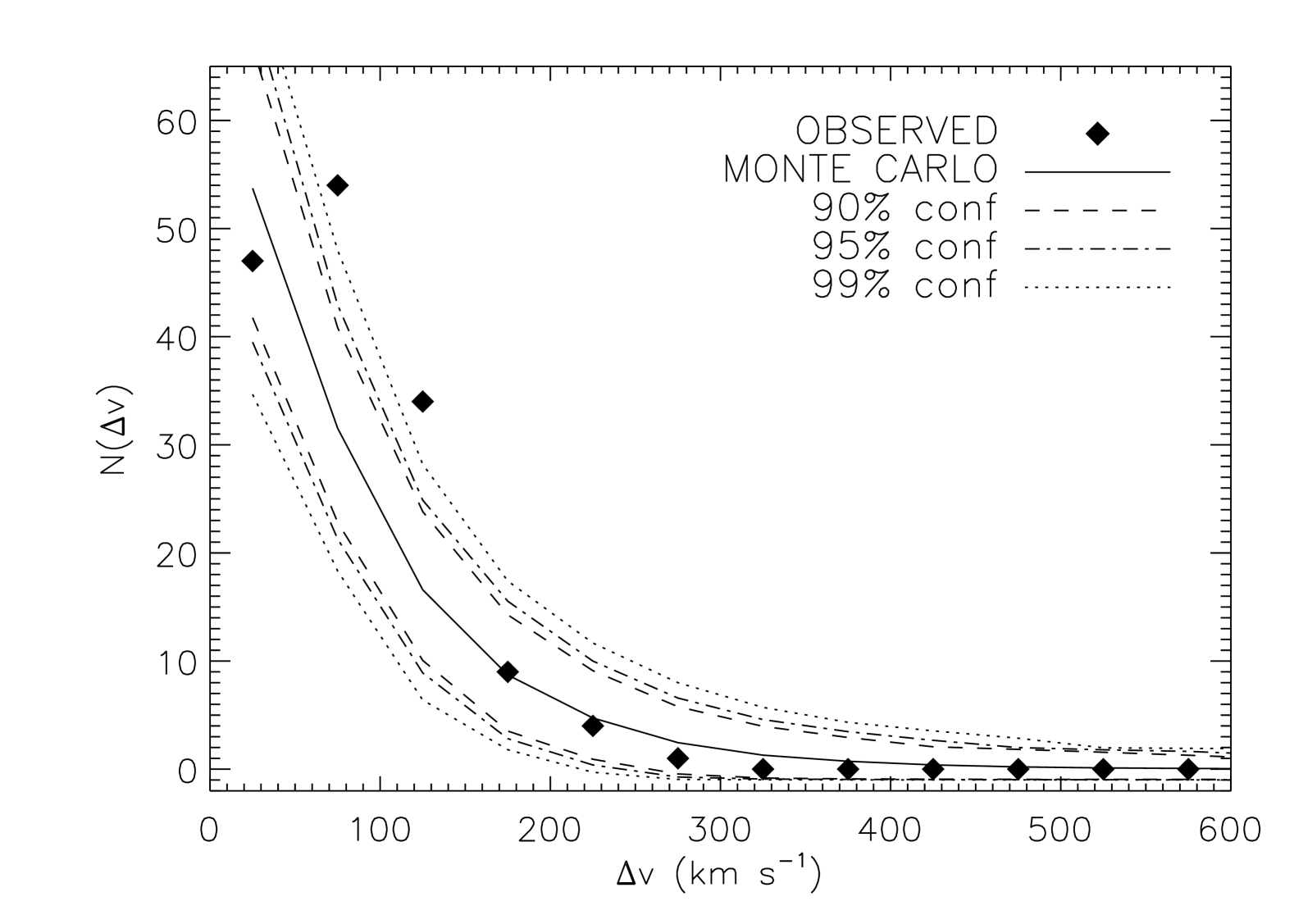
Figure 7.— The velocity splitting of 152 symmetrically matched pairs. The results of random matching Monte Carlo experiments are overplotted with 90$\%$, 95$\%$, and 99$\%$ confidence intervals. The first data bin, from 0-50 km s^-1, is significantly limited by the instrumental resolution and thus contains fewer matches than high resolution echelle spectra would exhibit. The 50-100 km s^-1 and 100-150 km s^-1 bins show a 3-4$\sigma$ coherence signal above the Monte Carlo expectation. Wider velocity splitting bins with $\Delta v>150$ km s^-1 follow expectation from random pairings.

Symmetric pair matches may just be chance pairings. The mean separation between matched pairs is 1.4Å or $\sim$84 km s^-1, as seen as a peak in Figure 7. In contrast, the average separation between adjacent lines in each individual spectrum (a measure of line density) is 6.1 $\pm$ 3.6Å ($\sim$370 km s^-1) in A and 6.8 $\pm$ 4.2Å ($\sim$410 km s^-1) in B. If the requirement of symmetry (A matches to B and B matches to A) is dropped in the matching process, the mean $\Delta\lambda$ increases as expected (to 3.4$\pm$6.5Å). To indicate the physical scale on which lines are being matched, we calculate the velocity scale of differential Hubble flow. Using an angular separation of 198″, a typical radial line separation translates to $\Delta\lambda_{o}$ = 4.5Å, or $\sim$270 km s^-1.

7.3. Monte Carlo Experiment

We perform a Monte Carlo experiment to test the significance of symmetric line matches, by making matches across sightlines as a way to detect coherence (above the chance matching resulting from randomly placed lines). This test is not limited or compromised by low resolution because lines are typically centroided to 30 km s^-1($\sim$0.5Å), which is $\sim$7 times smaller than our 220 km s^-1(3.6Å) resolution (Dinshaw et al., 1998, , using the same method for HST data of similar resolution). Since the line velocity error (30 km s^-1) is much less than the mean velocity splitting of matched pairs (84 km s^-1), the measurement error does not impact this line matching coherence measure. With 1000 realizations, the experiment recreates the two sightlines, sampled to mimic the line density and equivalent width distribution of the observed spectra, and computes symmetric matches between the two randomly drawn sets of absorbers. The entire range of the data is used, including the Ly$\beta$ forest. This adds needed line statistics to the Ly$\alpha$ sample, and since line fitting is somewhat immune from varying mean flux and continuum fits (which exhibit strange behavior in the Ly$\beta$ region as can be seen by excessive opacity in Figure 1, particularly in A) there is no concern that line matches in the Ly$\beta$ region are not meaningful. The only risk in including the Ly$\beta$ region is double counting Ly$\alpha$ and their Ly$\beta$ counterpart matches, which will also trace coherence in the IGM. This double counting is unlikely since we found very little evidence that Ly$\beta$ contamination is significant, and at most, would only change the result by $\sim$10$\%$.

To create the simulated Monte Carlo samples, we use the limiting equivalent width (or detection limit) as a function of wavelength, which hovers about 0.24Å. Damped regions are removed from the simulated spectra as from the data: 5005-5060Å in A and 5145-5160Å in B. We overplot the results of this Monte Carlo matching experiment on our observed matches in Figure 7. The data show a $\sim$4$\sigma$ coherence signal above the Monte Carlo random matching result in the 50-100 km s^-1 and 100-150 km s^-1 bins (pair excesses are 3.9$\sigma$ and 3.7$\sigma$ respectively). The experiment was repeated by splitting the sample into strong and weak lines (split at 0.5Å, roughly half the sample), but it did not show that coherence was more prevelent in either strong or weak absorbers. The first bin (0-50km s^-1) is depopulated due to line blending; few symmetric matches on small velocity splitting scales would be counted if blended features containing two absorbers correspond to single absorbers in the opposite sightline. Therefore, we do not claim that the offset signal (peak between 50 km s^-1 $<\Delta v<$ 150 km s^-1) is due to inherent shear in the IGM.

8. COMPARISON WITH THE SIMULATIONS

8.1. Absorber Coincidences from Simulations

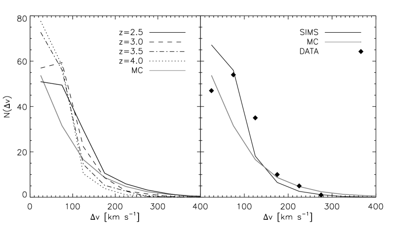
Figure 8.— The velocity splitting distribution of absorbers in the spectra extracted from the simulations. The left panel shows the distribution as a function of realization redshift. For reference, we have overplotted the random absorber result from Monte Carlo tests (as shown in Figure 7), and we see that the simulations show a weak but detectable coherence signal above random chance pairings. When properly weighted over the redshift interval of our data (2.6 $<$ z $<$ 3.8), we show the simulations alongside the data result and the random test result in the right panel.

To further interpret our $\sim$4$\sigma$ detection of coherence from the previous section, we perform a similar symmetric pair matching on absorbers in the spectra extracted from simulations (as described in §3). Line fitting was done with the same $ANIMALS$ utility that was used for the data, this time applied to the degraded extractions from simulations designed to match the data. Figure 8 (left panel) shows the velocity splitting distribution at each redshift for symmetrically matched pairs in associated A and B simulated spectra (with the MC randomization result overplotted for reference). At higher redshift, greater line densities generate a steeper peak at zero splitting as expected, while lower redshifts give shallower distributions. To make a fair comparison with the data, we interpolate the distribution shape that simulations would produce for a spectrum continuously sampling redshifts 2.6 $<$ z $<$ 3.8. This is shown alongside the randomized result and the data in the right panel of Figure 8. This not only reaffirms that we can detect weak coherence in the lya forest at high redshifts, but that the simulations agree with our data in showing a signal of roughly the same strength.

The one area of disagreement between data and degraded extractions from the simulations is in the first velocity offset bin (0-50km s^-1). This can be explained simply as a depopulation of the smallest velocity offset bin in the data due to line blending (i.e. the discrepancy is non-physical). Although this happens to some degree in the spectra extracted from simulations, the settings in $ANIMALS$ used to generate line lists from the simulations allow lines to be fitted with smaller wavelength separations (below the 0.85Å restriction applied to the data) since the spectra themselves are so short (only 300Å , rather than the data that span $\sim$1500Å). The lowest bin, where the turn-down occurs in the data, correponds to splittings less than 40$\%$ of the instrumental resultion. At these high redshifts, where blending is severe, the transverse matching result will be sensitive to the exact criterion used for minimum line separation in each sightline. The slight depopulation of simulation matched pairs relative to data at high velocity splitting is a consequence of the same effect. To first order, this preliminary test for high-z coherence is successful and it encourages additional testing of the simulations that can be done in the future more effectively using higher quality data.

8.2. Evolution in the Transmission Distribution

Figure 9.— The transmission distributions of 3000 spectra extracted from SPH simulations at four discrete redshifts. The first column shows the distributions of non-degraded simulation spectra, with no noise added and very high resolution, which characterizes the intrinsic cosmic evolution of the IGM in the simulations. The second column shows the distributions for simulations after degrading to the signal-to-noise and instrumental resolution of the spectra, but without rescaling the mean flux. The distributions of A and B do not differ despite a difference in SNR, so they are combined. The effect of resolution is particularly visible at high redshift. The third and fourth columns represent the same distributions from column 2 after being rescaled by mean flux according to P93 (Press, Rybicki, & Schneider, 1993) and K05 (Kirkman et al., 2005) respectively. The vertical lines in the three last columns represent the average transmission value of the fitted continua as described in §8.3.

The spectra extracted from the G6 simulation (§3) show significant changes in opacity distributions over the redshift range of our data. At their initial high resolution and infinite SNR, the transmission distributions show substantial absorption at higher redshift while very little at low redshift, the anticipated strong cosmic evolution from z = 2.6 to z = 3.8 (Lyman limit to Ly$\alpha$ emission in our data). The transmission distributions in the first column of Figure 9 combine the statistics of both A and B simulated sightlines, non-degraded and not rescaled to mean flux via either P93 or K05. At z = 2.5, the lowest redshift of simulation extractions, there is a strong peak at high transmission indicating little absorption relative to the true continua; the small tail at zero transmission indicates the number of pixels in damped systems. At higher redshifts, z = 3.0 and 3.5, there is a clear shift in the distribution towards lower transmission, and the z = 4.0 distribution suggests opacity at nearly every pixel. The number of opaque pixels increases tenfold from z = 2.5 to z = 4.0 from 3.1$\%$ to 20.0$\%$ of all pixels.

After degrading the raw extracted spectra to the signal-to-noise and resolution of the data, the second column of Figure 9 shows changes in the overall transmission distribution at each redshift. There was no observed SNR effect on transmission distributions shape, so the statistics from both fabricated sightlines were combined and weighted by relative SNR. The effects are as expected: the peaks have broadened, there are fewer pixels with zero transmission, and since noise has been added, a small fraction of pixels have transmission greater than one. With increasing redshift, the distribution shape evolves from a high transmission peak to a nearly linear fall off with higher transmission at z = 4.0. In the figure, the dotted line indicates zero opacity (the true continuum), and the dashed line indicates the average level of the continuum fit after the simulation extractions are degraded.

If the degraded simulations are altered to match the mean flux estimates given by P93 and K05 the transmission distributions change shape, as shown in the third and fourth columns of Figure 9. The P93 rescaled simulations have very similar shapes to the raw degraded simulations, while the K05 rescaled simulations do not show as much dramatic evolution at high redshift. This comparison shows the importance of mean transmission in interpreting data where it is not known a priori.

8.3. Underestimation in Continuum Flux

From the simulation, we infer a systematic error in $ANIMALS$ continuum fitting as a function of redshift. When degraded to the resolution of our observations, the smoothing of transmission on small velocity scales shifts the peak transmission values lower, and so depresses any algorithmic fit to the continuum. This effect becomes larger at higher redshifts as the mean opacity in the IGM increases. The vertical dashed lines on columns 2-4 of Figure 9 represent the transmission values of the fitted continuum (with respect to the true continuum level). When we compare the data’s transmission distributions to those of the simulation, we use the estimate of the continuum fit transmission to rescale the data’s flux, thus correcting the underestimation and making the comparison between data and simulation fair. The flux decrement of the continuum may be modeled as a parabolic function of $(1+z)$:

$$fd_{cont}(1+z)=0.697-0.419(1+z)+0.065(1+z)^{2}$$ (3)

with variance $\sigma_{fd}^{2}=0.002$, and valid for $2.5<z<4.0$. A quadratic fit is empirically chosen because a linear fit is an inappropriate choice to model such redshift evolution. The rescaling of degraded spectra to either P93 or K05 does not have any additional impact on the underestimation of continuum flux. Pixels that have very high or low transmission are not affected by rescaling the mean flux as much as pixels with intermediate absorption, and since the continuum fitting is based on the highest transmission pixels, the rescaling effect will be minimal, particularly at low redshift. At high redshift the size and uncertainty in the continuum underestimation grow as would the effect of rescaling by mean flux, but it is clear that the systematic error in the fit dominates the continuum flux value over the smaller variations between raw, P93, and K05 mean flux rescalings.

This systematic effect leads to an underestimation of line density as well as equivalent width. At high redshift, where the effect is most severe, only the strongest and highest column density features will be fit via $ANIMALS$ methods, while the much weaker lines in blended regions are not fit. The size of this effect cannot be properly measured since line fitting relative to the true continua is not a unique process when there is opacity at nearly every pixel. Echelle spectra can mitigate this problem, since moderately strong features will be fully resolved and reliably measured regardless of the true continuum level.

8.4. Comparisons of Transmission Distributions

When comparing the observational data to simulations we must recall that the SPH extractions represent discrete epochs (z = 2.5, 3.0, 3.5, and 4.0) while the data samples redshift continuously with cosmic evolution superimposed. We split the spectra into five bins $\sim$300Å wide, centered at redshifts 2.75, 2.99, 3.26, 3.47 and 3.67. These redshift bins were chosen to avoid problem areas in both spectra$-$the large damped system in quasar A (5005-5060Å), all data blueward of the Lyman limit in either spectrum ($\lambda>$4420Å), and all data redward of the DLAs close to the Ly$\alpha$ emission peaks ($\lambda<$5790Å). The first two bins, z = 2.75 and 2.99, cover the Ly$\beta$ forest while the three subsequent bins, z = 3.26, 3.47 and 3.67, cover the Ly$\alpha$ forest and are slightly narrower in width ($\sim 280$Å).

Figure 10.— Transmission distributions of combined data for both quasars split into five redshift bins centered at 2.75, 2.99, 3.26, 3.47, and 3.67. The distributions of spectra extracted from simulations are overplotted at these redshifts by linearly interpolating the transmission distribution shapes from the four extraction redshifts: 2.5, 3.0, 3.5, and 4.0. Press, Rybicki, & Schneider (1993) (dashed lines) and Kirkman et al. (2005) (solid lines) mean flux rescalings show quite different distribution shapes, particularly at high redshift. The data transmission was rescaled to correct for the systematic underestimation in the $ANIMALS$ continuum fit, as described in §8.3.

We linearly interpolate the shapes of the simulations’ transmission distributions to infer the distribution shape at these five intermediate redshifts. We do these procedures using both P93 and K05 sets of spectra, adopting different mean flux values for the simulations. Figure 10 shows the transmission distributions for the data (histogram) and the simulations (P93 scaling is dashed and K05 scaling is solid) at the five redshift bins. Since the continuum flux has a significant effect on transmission (particularly at high redshift), we rescale the normalized data flux by a factor representing the mean $ANIMALS$ fitted continuum flux (as a function of redshift). The transmission of each pixel in the data is rescaled by this continuum flux factor, given by equation 3, which removes the effect of the systematic underestimation in the continuum fit.

At the lowest redshift (z = 2.75 in Figure 10), the data show far more low transmission pixels than anticipated. The extra absorption relates directly to the excess in line density seen in Figure 5, but is too large an effect to be attributed directly to Ly$\beta$ absorbers or metal absorbers. Since the signal-to-noise of the blue end of the data is quite low, the true transmission distribution may be modified by a large flux error. The remaining four bins from 2.99 to 3.67 show fairly good agreement between simulations and data. To test agreement with the simulations models, both from the Kirkman et al. and Press et al. treatments, we performed K-S tests to test goodness of fit. It revealed that significant agreement ($>$45$\%$) only occured in the three highest redshift bins (z = 3.26, 3.47 and 3.67) using the Kirkman mean flux scaling simulations treatment (with probabilities of 48$\%$, 96$\%$, and 63$\%$ respectively). The lower redshift bins in the Kirkman treatment, and none of the Press, Rybicki, & Schneider (1993) transmission distributions were proper fits, all with probabilities lower than 3$\%$.

8.5. Transverse Correlation Comparison

Figure 11.— The distribution in cross-correlation amplitude for the simulations, with Kirkman et al. (2005) (top) and Press, Rybicki, & Schneider (1993) (bottom) mean flux rescalings. The 2000 simulations used for this experiment are split into four (uneven) redshift bins to reproduce the cleanest portions of observed spectra: $2.75<z<2.95$, $3.19<z<3.22$, $3.26<z<3.58$ and $3.59<z<3.75$. The first bin shown includes a portion of the Ly$\beta$ forest. The final two panels are combinations of the first four: ’ALL’ means it covers the entire range of our data (all four bins) and ’LYA’ represents the exclusive Ly$\alpha$ forest experiment, $z>3.19$ (excluding the lowest redshift bin). The dashed vertical lines indicate the cross-correlation measurements for the data.

To compute the cross-correlation between simulation sightlines, the extracted spectra are pieced together from the z = 3.0 and z = 3.5 realizations to cover the wavelength range of the data. Instead of using linear interpolation to account for evolution at intermediate redshifts, piecing together extraction spectra (300Å in length) from the discrete redshift bins (2.5, 3.0, 3.5, 4.0) is a better test of simulation and data agreement. Rather than measuring cross-correlation for each redshift and then interpolating, we meaasure the cross-correlation from spectra pieced together to model the redshift evolution. The spliced simulation spectra run from 4420Å (the Lyman limit in B) at the blue end to 3000 km s^-1 blueward of Ly$\alpha$ emission in A (5765Å). Portions of the spectra are masked due to features in the data: the damped system in A from 5005-5060Å, an emission feature in A from 5142-5148Å, and the 5575Å sky line. Since inclusion of the Ly$\beta$ forest region may not be warranted (see the discussion in §6.4), we perform cross-correlation in segments: from $2.75<z<2.95$ (the Ly$\beta$ region with $SNR>10$), $3.19<z<3.22$ (the Ly$\alpha$ forest between the damped feature and Ly$\alpha$ emission), $3.26<z<3.58$ (the Ly$\alpha$ forest between Ly$\alpha$ emission and the 5577Å sky line), and $3.59<z<3.75$. The results are then combined into two larger bins: the Ly$\alpha$ forest (all bins with $z>3.19$) and the entire range (including the lowest bin, which spans part of the Ly$\beta$ forest). The cross-correlations are computed for both P93 and K05 mean flux scalings. The distribution of the cross-correlation amplitudes for the simulations is shown in Figure 11. The top set of panels shows the results for Kirkman et al. (2005) mean flux rescalings while the bottom half show those for Press, Rybicki, & Schneider (1993). The cross-correlation amplitude is within 1-2$\sigma$ of zero in every case, which emphasizes the difficulty of measuring coherence at this physical separation and redshift, given sample variance. Overall, the experiment shows that the K05 rescaled simulations are correctly modeling the Ly$\alpha$ absorbers at high redshifts since the data measurements are consistently within $\sim$1$\sigma$ of the mean cross-correlation amplitude. On the other hand, simulations assuming rescaled flux according to Press, Rybicki, & Schneider (1993) do not agree with data, with a difference of $\sim$8$\sigma$ over the Ly$\alpha$ region. This agreement with Kirkman et al. (2005) rather than Press, Rybicki, & Schneider (1993) is consistent with the earlier result from transmission distributions in §8.4 (as seen in Figure 10).

9. SUMMARY

This paper has presented new spectroscopic observations of the $z\sim 3.8$, 198″ separation quasar pair PC 1643+4631A, B and associated detection of coherence in the IGM on scales that have not been previously tested, $\sim$2.5 $h^{-1}_{70}$ Mpc. The observations cover the full extent of the Ly$\alpha$ forest range from Ly$\alpha$ emission to the Lyman limit (with high signal-to-noise and moderate resolution, 3.6Å) and provide an excellent opportunity to not only measure coherence and large scale structure in the IGM at high redshift, but also compare observations with predictions from cosmological simulations.

The Ly$\alpha$ absorber sample was defined in two ways: using the entire range of data from Ly$\alpha$ emission to the Lyman limit, or restricting the Ly$\alpha$ experiment to the region between Ly$\alpha$ emission and Ly$\beta$ emission, dubbed the pure Ly$\alpha$ region. Metal and higher order Lyman lines were not detected in the Ly$\beta$ forest region due to the high line densities, but since contamination may be present and the blue wavelengths have low SNR we treat the Ly$\beta$ forest region separately from the Ly$\alpha$ forest in flux statistics studies. A Monte Carlo random pairing experiment using the entire range revealed that chance pairs account for a significant portion of the velocity splitting of symmetric matches, but in addition to that the data show a 4$\sigma$ excess of pairs relative to random, near zero velocity splitting ($\Delta v<150$ km s^-1). This shows that multiple sightline coherence techniques work using line counting when applied to high redshift quasar pairs, and produce significant detections of coherence on $\sim$ 2.5 $h^{-1}_{70}$ Mpc scales up to $z\sim 3.8$.

This data set have provided a unique opportunity to test expecations from simulations. The nearest-neighbor absorber matching, transmission distribution and transverse coherence all indicate agreement between simulation expectations and results from data, which has not been reliably tested before at this high redshift and wide separation, primarily since quasar pairs of this type are rare. The absorber matching experiment shows that the simulations show a weak but detectable coherence signal at low velocity splitting, with the same 4$\sigma$ strength as the data. Combining sightline statistics, we compared transmission distributions in five discrete bins and see that the data generally agree with the redshift evolution of the simulation’s transmission distribution shapes, and agree best with the Kirkman et al. (2005) treatment of mean flux rescaling. The cross-correlation experiment finds a weak coherence signal from the simulations for both mean flux decrements (Press et al., 1993; Kirkman et al., 2005); the data also show a weak signal when rescaled by Kirkman et al. (2005), agreeing with the simulation result, but show a strong coherence measurement if rescaled by Press, Rybicki, & Schneider (1993). These three separate statistics (arbsorber matching, transmission distribution shape and cross-correlation amplitude) are mutually consistent and have opened a new regime in redshift and wide separation on which to compare the structure of the IGM, and agreement between data and simulations.

References

- Bahcall et al. (1996) Bahcall, J. N., et al. 1996, ApJ, 457, 19
- Bechtold (1994) Bechtold, J. 1994, ApJS, 91, 1
- Bernardi et al. (2003) Bernardi, M., et al. 2003, AJ, 125, 32
- Cen et al. (1994) Cen, R., Miralda-Escudé, J., Ostriker, J. P., & Rauch, M. 1994, ApJ, 437, L9
- Cen & Simcoe (1997) Cen, R., & Simcoe, R. A. 1997, ApJ, 483, 8
- Croft et al. (1998) Croft, R. A. C., Weinberg, D. H., Katz, N., & Hernquist, L. 1998, ApJ, 495, 44
- Davé et al. (1999) Davé, R., Hernquist, L., Katz, N., & Weinberg, D. H. 1999, ApJ, 511, 521
- Davé & Oppenheimer (2007) Davé, R., & Oppenheimer, B. D. 2007, MNRAS, 374, 427
- Dinshaw et al. (1998) Dinshaw, N., Foltz, C. B., Impey, C. D., & Weymann, R. J. 1998, ApJ, 494, 567
- Fang & White (2004) Fang, T., & White, M. 2004, ApJ, 606, L9
- Finlator et al. (2006) Finlator, K., Davé, R., Papovich, C., & Hernquist, L. 2006, ApJ, 639, 672
- Finlator & Davé (2008) Finlator, K. & Davé, R. 2008, submitted to MNRAS
- Foltz et al. (1984) Foltz, C. B., Weymann, R. J., Roser, H.-J., & Chaffee, Jr., F. H. 1984, ApJ, 281, L1
- Haardt & Madau (1996) Haardt, F., & Madau, P. 1996, ApJ, 461, 20
- Hennawi et al. (2006) Hennawi, J. F., et al. 2006, ApJ, 651, 61
- Hernquist et al. (1996) Hernquist, L., Katz, N., Weinberg, D. H., & Miralda-Escudé, J. 1996, ApJ, 457, L51
- Hu et al. (1995) Hu, E. M., Kim, T.-S., Cowie, L. L., Songaila, A., & Rauch, M. 1995, AJ, 110, 1526
- Jannuzi et al. (1998) Jannuzi, B. T., et al. 1998, ApJS, 118, 1
- Jones et al. (1997) Jones, M. E., et al. 1997, ApJ, 479, L1
- Kim et al. (2001) Kim, T.-S., Cristiani, S., & D’Odorico, S. 2001, A&A, 373, 757
- Kim et al. (1997) Kim, T.-S., Hu, E. M., Cowie, L. L., & Songaila, A. 1997, AJ, 114, 1
- Kirkman et al. (2005) Kirkman, D., et al. 2005, MNRAS, 360, 1373
- Liske et al. (2000) Liske, J., Webb, J. K., Williger, G. M., Fernández-Soto, A., & Carswell, R. F. 2000, MNRAS, 311, 657
- Marble et al. (2007) Marble, A. R., Eriksen, K. A., Impey, C. D., Oppenheimer, B. D., & Davé, D. 2007, submitted to ApJ
- Murdoch et al. (1986) Murdoch, H. S., Hunstead, R. W., Pettini, M., & Blades, J. C. 1986, ApJ, 309, 19
- Oppenheimer & Davé (2006) Oppenheimer, B. D., & Davé, R. 2006, MNRAS, 373, 1265
- Petry et al. (2006) Petry, C. E., Impey, C. D., Fenton, J. L., & Foltz, C. B. 2006, AJ, 132, 2046
- Petry et al. (1998) Petry, C. E., Impey, C. D., & Foltz, C. B. 1998, ApJ, 494, 60
- Petry et al. (2002) Petry, C. E., Impey, C. D., Katz, N., Weinberg, D. H., & Hernquist, L. E. 2002, ApJ, 566, 30
- Press et al. (1993) Press, W. H., Rybicki, G. B., & Schneider, D. P. 1993, ApJ, 414, 64
- Rauch (1998) Rauch, M. 1998, ARA&A, 36, 267
- Rollinde et al. (2003) Rollinde, E., Petitjean, P., Pichon, C., Colombi, S., Aracil, B., D’Odorico, V., & Haehnelt, M. G. 2003, MNRAS, 341, 1279
- Sargent et al. (1980) Sargent, W. L. W., Young, P. J., Boksenberg, A., & Tytler, D. 1980, ApJS, 42, 41
- Saunders et al. (1997) Saunders, R., et al. 1997, ApJ, 479, L5
- Schaye (2001) Schaye, J. 2001, ApJ, 562, L95
- Schneider et al. (1991) Schneider, D. P., Schmidt, M., & Gunn, J. E. 1991, AJ, 101, 2004
- Scott et al. (2000) Scott, J., Bechtold, J., Dobrzycki, A., & Kulkarni, V. P. 2000, ApJS, 130, 67
- Shaver et al. (1982) Shaver, P. A., Boksenberg, A., & Robertson, J. G. 1982, ApJ, 261, L7
- Shaver & Robertson (1983) Shaver, P. A., & Robertson, J. G. 1983, ApJ, 268, L57
- Smette et al. (1995) Smette, A., Robertson, J. G., Shaver, P. A., Reimers, D., Wisotzki, L., & Koehler, T. 1995, A&AS, 113, 199
- Smette et al. (1992) Smette, A., Surdej, J., Shaver, P. A., Foltz, C. B., H., F., Weymann, R. J., Williams, R. E., & Magain, P. 1992, ApJ, 389, 39
- Spergel et al. (2003) Spergel, D. N., et al. 2003, ApJS, 148, 175
- Springel & Hernquist (2003) Springel, V., & Hernquist, L. 2003, MNRAS, 339, 312
- Springel et al. (2001) Springel, V., Yoshida, N., & White, S. D. M. 2001, New Astronomy, 6, 79
- Weymann & Foltz (1983) Weymann, R. J., & Foltz, C. B. 1983, ApJ, 272, L1
- Weymann et al. (1998) Weymann, R. J., et al. 1998, ApJ, 506, 1
- Williger et al. (2000) Williger, G. M., Smette, A., Hazard, C., Baldwin, J. A., & McMahon, R. G. 2000, ApJ, 532, 77
- Zhang et al. (1995) Zhang, Y., Anninos, P., & Norman, M. L. 1995, ApJ, 453, L57