Effective Viscosity of Dilute Bacterial Suspensions: A Two-Dimensional Model

Abstract

Suspensions of self-propelled particles are studied in the framework of two-dimensional (2D) Stokesean hydrodynamics. A formula is obtained for the effective viscosity of such suspensions in the limit of small concentrations. This formula includes the two terms that are found in the 2D version of Einstein’s classical result for passive suspensions. To this, the main result of the paper is added, an additional term due to self-propulsion which depends on the physical and geometric properties of the active suspension. This term explains the experimental observation of a decrease in effective viscosity in active suspensions.

1 Introduction

Recently there has been considerable interest in understanding the dynamics of systems of active interacting biological agents (active systems, for short), such as flocking birds, schooling fish, swarming bacteria, etc [1, 2, 3, 4, 5, 6]. Properties of these strongly self-organizing dissipative systems are of fundamental interest to nonequilibrium statistical dynamics [7, 8, 9, 10, 12] and to potential technological applications [13].

Common swimming (motile) bacteria, such as Bacillus Subtilis, Escherichia coli, and many others, are rod-shape microorganisms (length about 5 $\mu m$, diameter of the order 1 $\mu m$), propelled by the input of mechanical energy at the smallest scales by the rotation of helical flagella attached to the cell wall. Suspensions of swimming bacteria (active suspensions) are a convenient representative of self-organizing biological systems. At relatively high filling fractions of bacteria, they interact mostly through hydrodynamic entrainment induced by their swimming with respect to ambient fluid [4, 14], which are instrumental in the establishment of long-range order. At the same time, they are amenable to accurate experimental studies, control, and manipulation [14]. In the dense regime, the dynamics of active suspensions is dominated by the multiple body interactions and long-range self-organized coherent structures, such as recurring whorls and jets with the spatial scale exceeding the size of individual bacterium by an order of magnitude. This, however, makes the analysis rather challenging.

In the dilute regime, the hydrodynamic interactions between bacteria (or passive particles) are often ignored as the interparticle distance exceeds the range of the flows resulting from the particle motion. Therefore, in this case it is possible to isolate the effect of the particle-fluid interactions on the effective properties of active suspensions. This constitutes a step towards the full understanding and utilization of the novel properties of active suspensions.

The first step was taken in [15] by Einstein, who derived an explicit formula for the effective viscosity of a dilute suspension of passive spheres. This formula shows an increase of the viscosity over that of the ambient fluid alone. The correction to the effective viscosity is to the first order in the volume fraction of the inclusions. Later, Batchelor and Greene obtained the second order asymptotic formula, which takes into account pairwise interactions between particles [16]. Jeffrey calculated the effective viscosity of a suspension of ellipsoidal particles to first order in [17]. Unlike the spherical case, here the value of the viscosity is affected by the distribution of orientations of the inclusions, which is assumed to be uniform.

In this work, Einstein’s classical dilute limit result is extended to the case of self-propelled disk inclusions in a 2D Stokesean fluid. The choice of two-dimensional hydrodynamics is motivated by the tractable nature of calculations involving Green’s functions in 2D and also by the quasi-two-dimensional thin film geometry of the experiment [14]. In particular, the correction to the effective viscosity is explicitly calculated as a function of the orientations of the bacteria’s flagella, the intensity of the their force of self-propulsion, and the volume fraction of the suspension. In the case of an absence of self propulsion and, alternatively, the case of a uniform distribution of orientations, the result recovers the 2D version of Einstein’s result (see, e.g.[18]).

The model of the bacterium and the corresponding hydrodynamics are described in Section 2. Following Batchelor [19], the effective viscosity of a dilute suspension is defined in Section 2, in terms of a suitable background flow and the disturbance flow produced by the inclusion of a bacterium in the background flow. In the case of self-propulsion the disturbance flow is due both to the passive response of the background flow to the inclusion of a particle as well as the response of the stationary fluid to the particle’s self-propulsion. Because of the linearity of Stokesean hydrodynamics, the two components of the disturbance flow can be computed independently using the Green’s function for the disk.

The disturbance flow $u_{p}^{\prime}$ due to the locomotion of a single bacterium is calculated in Section 3. This flow translates the bacterium. It is also shown that this disturbance flow decays at infinity. This result is emphasized since it is a point of well-known deficiency of 2D hydrodynamics. Indeed, while the translation of a ball in 3D produces no flow at infinity, in the well-known Stokes paradox, the 3D flow due to an infinite cylinder (described by the corresponding force monopole) translating transversely to its axis generates a non-zero flow at infinity (see, e.g., [21]). Thus prevents the decoupling of rods, which is needed for the dilute limit, where it is assumed that the flow due to a suspension can be approximated by the sum of solutions due to a single inclusion. However, a self-propelled particle is constrained by the viscous drug force opposing the propulsion force, thus producing a force dipole which decays at infinity, unlike the force monopole in the case of the moving disk.

For the other disturbance flow, $u_{int}^{\prime}$, due to the bacterium’s passive response to a background flow, care must be taken to ensure that no flow is produced at infinity. Thus, in Section 4 such a flow is selected to ensure the disturbance decays at infinity. Once it has been done, the effective viscosity is calculated as a function of the flagella’s orientations relative to the background flow. The time-dependent nature of the effective viscosity, due to active alignment of the inclusions to the flow, is also discussed. Conclusions are discussed in Section 5. Finally, the details of calculations are discussed in the appendices.

2 Model and its Homogenization

A 2D dilute suspension of bacteria is modeled as a collection of discs of radius $a$, each of which has an associated point force, representing the flagellum, placed at a distance $\lambda a$ from the disk, as shown in Figure 1. The point force is directed radially outward from the center of the bacterium and has some orientation angle $\alpha$, measured from the $x$-axis. The bacteria are distributed throughout an ambient fluid of viscosity $\eta$ which takes up the entire domain $\mathbb{R}^{2}$. A single bacterium in an infinite fluid moves with respect to the fluid with constant velocity driven by the point force $\vec{c}$.

The suspension is assumed to contain sufficiently many bacteria so as to produce appreciable changes in the properties of the equivalent homogenized fluid. At the same time, the size of the bacteria and the propulsion force are assumed to be sufficiently small, so that the disturbance flow produced by bacteria is negligible at inter-bacterial distances and hence can be ignored at the locations of other bacteria. Therefore, in the following calculations, it is sufficient to consider a single bacterium with orientation $\alpha$ in an unbounded volume of fluid. This is analogous to Einstein’s assumptions for passive suspensions.

This unbounded volume is an idealization of the microscopic volume element surrounding a single one of the particles located within a macroscopic fluid element. Because of the decay assumption, this idealization is permissible for the solution of the Stokes’ equation within that region. The viscous dissipation in the macroscopic fluid element is then the sum of the dissipations in all of the subordinate microscopic volumes, containing a collection of particles having some prescribed distribution of orientations. Analogous to the method of Batchelor in [19], the effective viscosity $\eta^{*}$ of a suspension in an ambient fluid of viscosity $\eta$ is defined as the viscosity of an equivalent fluid with no inclusions that produces the same energy dissipation in each macroscopic volume element.

For a suspension of passive particles, the existence of an equivalent Newtonian fluid with the scalar effective viscosity $\eta^{*}$ is a classical result of homogenization theory (see e.g., [20] and references therein). The analysis for active particles is more subtle and has not been carried out in a rigorous mathematical context. The assumption is made that the effective viscosity can be defined in the same way for active particles. Nevertheless, the technique is presented somewhat cryptically in the literature. To clarify the main points, the conceptual side of the calculation is presented here in some detail; the technical details can be found in A (also see [19] for the derivation in the case of passive particles).

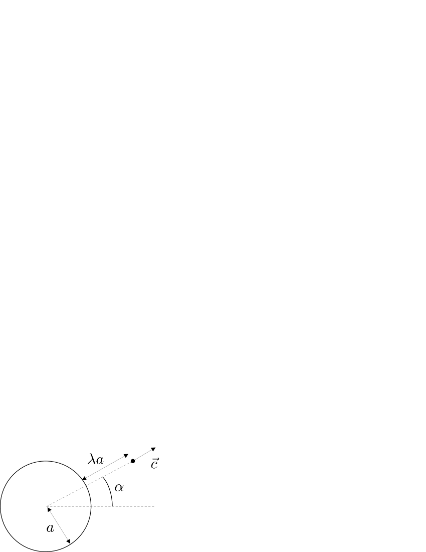
Figure 1: Schematic presentation of a bacterium with orientation $\alpha$.

Since the effective viscosity is defined in terms of energy dissipation, a background flow (which describes the flow throughout the homogenized fluid and on the boundary of the suspension) is chosen so that it has a non-zero rate of energy dissipation (i.e., requiring a non-zero strain rate). Choosing $\mathbb{R}^{2}$ to represent the microscopic volume with coordinates $\{x_{i}\},\ i=1,2$ the velocity components of the background flow are $u_{i}=\epsilon_{ij}x_{j}$, where $\epsilon_{ij}$ is constant and symmetric strain rate tensor but otherwise left to be specified later. Adding a single self-propelled disk inclusion $V_{b}$ somewhere in the plane produces the disturbance flow $\vec{u}^{\prime}$. Provided that $\vec{u}$ is selected properly, $\vec{u}^{\prime}$ vanishes at infinity, decoupling the bacteria, as required of the dilute limit. The disturbance flow can be computed explicitly and it is done below. The total flow of the suspension is $\vec{\tilde{u}}=\vec{u}+\vec{u}^{\prime}$ and in principle it should be possible now to compare the dissipation rates of $\vec{u}$ and $\vec{\tilde{u}}$ by integrating over $\mathbb{R}^{2}$ and $\mathbb{R}^{2}-V_{b}$ respectively.

As shown in [19], the integration over the unbounded volume $\mathbb{R}^{2}$ leads to technical difficulties. This motivates the more efficient method of comparing the dissipation rates within a bounded domain $\tilde{V}$ which contains sufficiently many bacteria. Figure 2 shows such a domain encompassing two bacteria. Inside $\tilde{V}$ are the regions representing the bodies of the bacteria, $V_{B_{l}}$ and, for each, an $\varepsilon$-disk $V_{\varepsilon,l}$ around the corresponding point force. The disturbance flow in the domain $\tilde{V}-\sum_{l}V_{B_{l}}-\sum V_{\varepsilon,l}$ is required to vanish at the outer boundary $\tilde{\Gamma}=\partial\tilde{V}$.

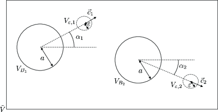
Figure 2: Bounded domain $\tilde{V}$ for which the modified dissipation rate is computed; includes the complement of two $a$-disks (bacteria) and $\varepsilon$-disks (neighborhoods of point forces).

This models a finite container with the background flow applied at the boundary and simplifies the computation of the dissipation rate integrals by replacing a volume integral with an integral over the boundaries of the bacteria.

Calculating the disturbance flows $\vec{u}^{\prime}$, however, involves solving a boundary value problem in the two-dimensional domain $\tilde{V}-\sum_{l}V_{B_{l}}-\sum V_{\varepsilon,l}$. To avoid this, the total dissipation rate in this domain can be equivalently calculated as the integral of the work of forces at the boundary $\tilde{\Gamma}$. By requiring that $u^{\prime}$ vanish at $\Gamma=\partial V$, the flow of the homogenized fluid and total flow of the suspension agree on the boundary $\Gamma$, $u_{i}=\tilde{u}_{i}=\epsilon_{ij}\,x_{j}$, but the corresponding values of the stress tensors $\sigma$ and $\tilde{\sigma}$ are not necessarily the same. Now, the density of work at the boundary is $n_{i}\sigma_{ij}\epsilon_{jk}x_{k}$ and $n_{i}\tilde{\sigma}_{ij}\epsilon_{jk}x_{k}$ for the homogenized and total suspension flows respectively. The effective viscosity is defined by integrating these quantities over $\Gamma$ and setting them equal:

$$\int_{\Gamma}\sigma_{ij}u_{i}n_{j}dA=\int_{\Gamma}\tilde{\sigma}_{ij}\tilde{u}_{i}n_{j}dA.$$ (1)

Using the Stokes equation $\nabla\cdot\sigma^{\prime}=0$ and repeatedly applying the divergence theorem (see appendix A), the integrals of these densities over $\tilde{\Gamma}$ can be reduced to integrals over the boundary of the bacterial domain only: $\Gamma_{b}+\Gamma_{\varepsilon}=\partial V_{b}+\partial V_{\varepsilon}$. These integrals are independent of $\tilde{\Gamma}$ and upon passing to the limit $\tilde{V}\longrightarrow\mathbb{R}^{2}$ they are expressed in terms of the disturbance flow $\vec{u}^{\prime}$ vanishing at infinity.

The effective viscosity is then determined from the expression resulting from summing over all inclusions:

$$2(\eta^{*}-\eta)\epsilon_{ij}\epsilon_{ij}$$

$$=\frac{\epsilon_{ik}}{A}\sum_{l}\int_{\partial V_{B_{l}}\cup\partial V_{\varepsilon,l}}\left(\sigma^{\prime}_{ij}x_{k}n_{j}-2\eta u^{\prime}_{i}n_{k}\right)dA.$$

Applying the dilute assumption, the solution to (28) is replaced by a superposition of solutions for the flow due to a single bacterium, derived in the next section. Thus, for aligned bacteria, the above integral can be replaced with one over the boundary of one bacterium in $\mathbb{R}^{2}$,

$$2(\eta^{*}-\eta)\epsilon_{ij}\epsilon_{ij}=$$

$$\epsilon_{ik}\phi\int_{\partial V_{B}\cup\partial V_{\varepsilon}}\left(\sigma^{\prime}_{ij}x_{k}n_{j}-2\eta u^{\prime}_{i}n_{k}\right)dA,$$

where $\phi$ is the volume fraction occupied by bacteria.

3 Flow due to a single bacterium

Let $\Omega$ be the exterior of the unit disk in $\mathbb{R}^{2}$ and $\delta_{\vec{r}_{0}}$ be the Dirac delta evaluated at $\vec{r}-\vec{r}_{0}$, where $\vec{r}_{0}$ is the location of the point force. In the low Reynolds number limit, the flow due to the bacterium obeys the Stokes equation

$$\left\{\begin{array}[]{rl}\eta\Delta\vec{u_{p}^{\prime}}&=\nabla p_{p}^{\prime}+\vec{c}\delta_{\vec{r}_{0}}\text{ in }\Omega\\ \nabla\cdot\vec{u}_{p}^{\prime}&=0\text{ in }\Omega\\ \vec{u}_{p}^{\prime}&=0\text{ on }\Gamma\end{array},\right.$$ (4)

where $\vec{c}$ is the force strength and $\Gamma=\partial\Omega$. For simplicity of calculations, set $\vec{c}=c\hat{e}_{1}$ and $\vec{r}_{0}=(1+\lambda)\hat{e}_{1}$. Note that here, $\vec{u}_{p}^{\prime}$ is set to $0$ on $\Gamma$. This is the reference frame in which the bacterium is moving–for the purpose of finding the total flow of the suspension, the reference frame in which the fluid is at rest at infinity must be used.

By writing $\vec{u}$ as the curl of a stream function $\Phi$ and taking the divergence of (4), this reduces to the inhomogeneous biharmonic equation

$$\left\{\begin{array}[]{c}\Delta^{2}\Phi(x,y)=\frac{\partial}{\partial y}\frac{c}{\eta}\delta_{\vec{r}_{0}}\text{ in }\Omega\\ \Phi=\frac{\partial\Phi}{\partial n}=0\text{ on }\Gamma\end{array}.\right.$$ (5)

The Green’s function $G$ for the domain $\Omega$ with these boundary conditions is known and yields the solution

$$\Phi(x,y)=-\frac{c}{\eta}\frac{\partial G}{\partial\gamma}(x+iy,1+\lambda).$$ (6)

Explicitly, in polar coordinates,

$$\Phi(r,\theta)=$$

$$\frac{cr\cos(\theta)}{8\pi\eta}\left[\frac{((1+\lambda)^{2}-1)(r^{2}-1)}{1+(1+\lambda)^{2}r^{2}-2(1+\lambda)r\cos(\theta)}\right.$$

$$\left.+\log\left(\frac{(1+\lambda)^{2}+r^{2}-2(1+\lambda)r\cos(\theta)}{1+(1+\lambda)^{2}r^{2}-2(1+\lambda)r\cos(\theta)}\right)\right].$$

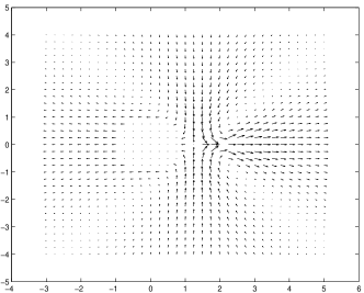
Figure 3: Velocity field produced by a bacterium in 2D geometry.

It is easy to see that $u_{p}^{\prime}\rightarrow u_{\infty}=\text{const.}$ as $r\rightarrow\infty$. Subtracting this flow (moving to the reference frame where the water is at rest at $\infty$) and rescaling to a disk of radius $a$, is shown in figure 3 and is given asymptotically by

$$\vec{u}(r,\theta)=$$ (8)

$$\left(\begin{array}[]{c}\frac{ca^{2}\lambda^{2}(2+\lambda)^{2}}{8\pi\eta(1+\lambda)^{3}}\frac{1}{r}(\cos(\theta)+\cos(3\theta))+O(\frac{1}{r^{2}})\\ \frac{ca^{2}\lambda^{2}(2+\lambda)^{2}}{8\pi\eta(1+\lambda)^{3}}\frac{1}{r}(\cos(2\theta)\sin(\theta))+O(\frac{1}{r^{2}})\end{array}\right).$$ (11)

Now, by taking the divergence of (4), one obtains

$$\left\{\begin{array}[]{rl}\Delta p&=-c\frac{\partial}{\partial x}\delta_{\vec{r}_{0}}\text{ in }\Omega\\ \nabla p\cdot\hat{n}&=\eta\Delta\vec{u}\cdot\hat{n}\text{ on }\Gamma\end{array}.\right.$$ (12)

The solution to (12) is found using complex function theory (see appendix D), and is the real part of the complex function

$$\Pi(z)=-\frac{c}{2\pi}\frac{a^{2}\lambda^{2}(2+\lambda)^{2}z}{(1+\lambda)(a(1+\lambda)-z)((1+\lambda)z-a)^{2}}.$$ (13)

4 Calculating the effective viscosity

In order to calculate the effective viscosity, it remains to perform the integration in (2). The effective viscosity is independent of the background flow, so one is free to choose the flow which simplifies the necessary calculations. In (2), $\vec{u}^{\prime}$ and $p^{\prime}$ are the solutions to

$$\left\{\begin{array}[]{l}\eta\Delta\vec{u}^{\prime}=\nabla p^{\prime}+\vec{c}\delta_{\vec{r}_{0}}\\ \nabla\cdot\vec{u}^{\prime}=0\end{array}\right.$$ (14)

subject to the boundary conditions

$$\begin{array}[]{ll}u^{\prime}_{i}\rightarrow\epsilon_{ij}x_{j}&\text{as }r\rightarrow\infty\\ \vec{u}^{\prime}=const&x\in\Gamma.\end{array}$$ (15)

Note that, as mentioned in section 3, one is not free to choose the value of the constant that $\vec{u}$ takes on $\Gamma$.

The formula for the effective viscosity does not depend on the choice of background flow (i.e., the choice of the strain rate tensor $\epsilon_{ij}$ in (15)). However, the choice of this flow is not completely arbitrary. First, since the effective viscosity is defined in terms of energy dissipation, a non-zero rate of strain is required so that there is energy being dissipated due to viscosity. Second, the background flow is chosen so that it does not rotate bacteria, which allows for the computation of the effective viscosity for a fixed (time-independent) distribution of orientations of bacteria (see figure 1). Third, upon placing a disk (i.e., bacterium) in the flow, it is necessary that the disturbance flow $\vec{u}_{int}^{\prime}\rightarrow 0$ as $r\rightarrow\infty$. If this were not the case, the dilute assumption that this flow is negligible at the locations of other bacteria would be violated. In 2D, this is only possible for a background flow that satisfies the conditions for existence of such a decaying flow derived in [22]. The background flow is chosen to be the simplest flow that matches these criteria–the sum of two perpendicular shearing flows,

$$\epsilon=2\epsilon_{0}\left(\begin{array}[]{cc}0&1\\ 1&0\end{array}\right).$$ (16)

where $\epsilon_{0}=const$ is the amplitude of the strain rate.

The disturbance flow due to the presence of a bacterium will be

$$\vec{u}^{\prime}=\vec{u}_{p}^{\prime}(\alpha)+\vec{u}_{int}^{\prime}$$ (17)

with the pressure given by

$$p^{\prime}=p_{p}^{\prime}(\alpha)+p_{int}^{\prime}$$ (18)

where, using notation, $\vec{u}_{p}^{\prime}(\alpha):=\vec{u}_{p}^{\prime}(r,\theta-\alpha)$ as a polar vector and $p_{p}^{\prime}(\alpha):=p_{p}^{\prime}(r,\theta-\alpha)$, rotated to allow for an arbitrary orientation of a bacterium in the background flow.

For a suspension of bacteria that are not fully aligned, the effective viscosity can be written in terms of the function $X(\alpha)$ which gives the probability density of orientations of the bacteria $\alpha_{l}$, which are assumed to be independent identically distributed random variables. In this case, (2) becomes

$$2(\eta^{*}-\eta)\epsilon_{ij}\epsilon_{ij}=$$

$$\epsilon_{ik}\phi\int_{0}^{2\pi}\int_{\partial V_{B}\cup\partial V_{\varepsilon}}\left(\sigma^{\prime}_{ij}(\alpha)x_{k}n_{j}\right.$$

$$\left.-2\eta u^{\prime}_{i}(\alpha)n_{k}\right)dAX(\alpha)d\alpha,$$

where $\phi$ is the volume fraction occupied by bacteria. Performing the integration over $\partial V_{B}\cup\partial V_{\varepsilon}$, one obtains the following formula for the effective viscosity:

$$\eta^{*}=\eta\left[1+2\phi\right.$$

$$\left.+\frac{c}{2\pi\eta\epsilon_{0}}\frac{1+2\lambda(2+\lambda)}{(1+\lambda)^{3}}\phi\int_{0}^{2\pi}\sin\left(2\alpha\right)X(\alpha)d\alpha\right],$$

where $\phi$ is the two-dimensional volume fraction.

Note that for isotropically oriented bacteria ($X(\alpha)=1/2\pi=const$), the angular term goes to zero and the effective viscosity reduces to the result in [18] for the effective viscosity of a two-dimensional dilute suspension of disks,

$$\eta^{*}=\eta\left(1+2\phi\right).$$ (21)

Nevertheless, in experiments a reduction in viscosity is anticipated [23]. In reality, bacteria are not spherical. An interaction with the background flow thus produces a torque on the bacteria which will tend to align them in particular preferred directions (see e.g. [24]). For a fully aligned suspension of bacteria, one obtains, from (4),

$$\eta^{*}=\eta\left[1+2\phi+\frac{c}{2\pi\eta\epsilon_{0}}\frac{1+2\lambda(2+\lambda)}{(1+\lambda)^{3}}\phi\sin 2\alpha\right].$$ (22)

For the background flow (16), the corresponding preferred directions are $\alpha=-\frac{\pi}{4},\frac{3\pi}{4}$. Thus, after aligning,

$$\eta^{*}=\eta\left[1+2\phi-\frac{c}{2\pi\eta\epsilon_{0}}\frac{1+2\lambda(2+\lambda)}{(1+\lambda)^{3}}\phi\right].$$ (23)

This formula can be used to explain the experimental data on the reduction of viscosity in bacterial suspensions observed in [14].

5 Conclusion

Here a rather puzzling result has been obtained: the effective viscosity of active bacterial suspension may decrease with the increase in volume fraction of particles. Moreover, the viscosity may even become formally negative (when the flagella add more energy than is being dissipated) if the volume fraction $\phi$ and the magnitude of the propulsion force $c$ exceed critical values. Manifestations of negative viscosity have been observed in experiments [14] via large-scale instability and the formation of non-decaying whorls and jets of collective locomotion (see also simulations [26, 27] for dense suspensions). The reduction of effective viscosity can be interpreted as a result of transformation by swimming bacteria of chemical energy of the surrounding nutrient medium into mechanical energy of fluid motion, and thus replacing energy loss due to viscous dissipation.

It is also notable that the coefficient $\epsilon_{0}$, which characterizes the strength of the background flow, shows up in the formula for effective viscosity (unlike in a Newtonian fluid). Thus, the additional term due to self-propulsion is inherently non-Newtonian. Since $\epsilon_{0}$ appears in the denominator, there is a blow up in the effective viscosity as $\epsilon_{0}\rightarrow 0$. Nevertheless, this is to be expected, as the viscosity is, roughly, the ratio of stress of the entire flow to rate of strain of the background flow–in the case of a bacterial suspension, as the rate of strain of the background flow goes to zero, the stress does not, since the bacteria will continue swimming.

We also comment that the limit of vanishing background flow $\epsilon_{0}\to 0$ is not trivial. As mentioned above, the reduction of viscosity occurs only when the bacteria become aligned in a certain direction determined by the principal axis of the strain-rate tensor. However, when $\epsilon_{0}\rightarrow 0$, the bacteria no longer have a tendency to align (also, a preexisting aligned state would be destroyed by fluctuations, e.g. due to random tumbling of bacteria) and hence the third term in Eq. (4) does not blow up. Thus, in the limit of $\epsilon_{0}\to 0$, the steady state is in fact the isotropically oriented suspensions $X(\alpha)=1/2\pi$, which recovers the classical result for disks Eq. (21). Moreover, since the effective viscosity for small strain rates is determined by the interplay between the response of the bacterium, through its orientation, to the shear strain and random fluctuations, one needs to solve self-consistently the equation for the orientation distribution function $X(\alpha$) in the presence of non-zero strain rate. This isotropic orientation can also explain the results of recent simulations [28] in which no reduction of the effective viscosity due to swimming bacteria (modeled by spherically symmetric particles) was detected: the reduction of viscosity requires particle reorientation by shear flow. However, the orientation of spherical particles is not affected by shear flow. In contrast, the effect is expected for elongated particles (ellipsoids or cylinders with large aspect ratios (of the order of 1:5 for swimming bacteria).

Obviously, more dedicated controlled experiments with bacterial suspensions and further generalizations of the obtained result to more general flow geometries, such as three-dimensional films and slabs, are keenly needed. The puzzling phenomenon of reduced viscosity in bacteria-laden fluids may find rather unexpected technological applications in bio-medical research and chemical technology, such as microscopic bacterial mixers and chemical reactors [13].

Acknowledgments

The work of L. Berlyand was partially supported by NSF grant DMS-0708324. I.S. Aranson and D. Karpeev were supported by US DOE, grant DOE grant DE-AC02-06CH11357.

Appendix A Calculation of Dissipation Rate and Definition of Effective Viscosity

Following [19], the rate of work being done at the boundary $\Gamma=\partial\Omega$ is given by

$$\int_{\Gamma}\sigma_{ij}u_{i}n_{j}dA=e_{ik}\int_{\Gamma}(-P\delta_{ij}+2\eta e_{ij})x_{k}n_{j}dA,$$ (24)

where $\sigma_{ij}$ is the stress tensor, $u$ is the velocity of the fluid, $n$ is the unit outward normal for the surface $\Gamma$, $P$ is the pressure of the fluid, and $e_{ij}$ is the rate of strain tensor. Henceforth, primed quantities will denote the disturbance values due to the presence of a bacterial suspension. The new stress tensor can be expressed as $\tilde{\sigma}_{ij}=\sigma_{ij}+\sigma^{\prime}_{ij}$. Additionally, on $\Gamma$, $e_{ij}=\epsilon_{ij}$. Thus, the effective viscosity of the suspension $\eta^{*}$ is defined by setting

$$\epsilon_{ik}\int_{\Gamma}(-P\delta_{ij}+2\eta^{*}\epsilon_{ij})x_{k}n_{j}dA=$$

$$\epsilon_{ik}\int_{\Gamma}(-P\delta_{ij}+2\eta\epsilon_{ij}+\sigma^{\prime}_{ij})x_{k}n_{j}dA.$$

Noting that the terms involving $P$ are identical on both sides and employing the divergence theorem yields

$$2A(\eta^{*}-\eta)\epsilon_{ij}\epsilon_{ij}=\epsilon_{ik}\int_{\Gamma}\sigma^{\prime}_{ij}x_{k}n_{j}dA,$$ (26)

where $A$ is the area of the surface $\Gamma$. The right hand side of (26) is the additional rate of dissipation due to the suspension. Employing the divergence theorem yet again, this integral is transformed into an integral over the surfaces of the particles, producing

$$\epsilon_{ik}\int_{\Gamma}\sigma^{\prime}_{ij}x_{k}n_{j}dA=$$

$$\epsilon_{ik}\int_{\Omega-\sum V_{B}\cup V_{\epsilon}}\left(\frac{\partial\sigma^{\prime}_{ij}}{\partial x_{j}}x_{k}+\sigma^{\prime}_{ik}\right)dV$$

$$+\epsilon_{ik}\sum\int_{\partial V_{B}\cup\partial V_{\epsilon}}\sigma^{\prime}_{ij}x_{k}n_{j}dA,$$

where $V_{B}$ is the volume occupied by a single bacterium, $V_{\epsilon}$ is a ball of radius $\epsilon$ around its corresponding point force, and the summation is taken over all bacteria inside $\Omega$. Now, the fluid in $\Omega$ obeys the inhomogeneous Stokes equation

$$\left\{\begin{array}[]{rlcc}\eta\Delta\vec{u}^{\prime}&=\nabla p^{\prime}+\sum_{l}\vec{c}_{l}\delta_{\vec{r}_{l}}&&\text{in }\Omega-\sum_{l}V_{B_{l}}\\ \nabla\cdot\vec{u}^{\prime}&=0&&\text{in }\Omega-\sum_{l}V_{B_{l}}\\ \vec{u}^{\prime}&=\vec{v}_{l}&&\text{on }\partial V_{B_{l}}\\ \vec{u}^{\prime}&=\epsilon_{ij}x_{j}&&\text{on }\partial\Omega\end{array},\right.$$ (28)

where the subscript $l$ has been added to all quantities that can vary among the bacteria. In particular, $\vec{v}_{l}$ is its velocity of the $l$th bacterium, $\vec{r}_{l}$ is the location of its point force, and $\vec{c}_{l}$ indicates the strength and orientation of each point force. Thus, $\frac{\partial\sigma^{\prime}_{ij}}{\partial x_{j}}=0$ in $\Omega-\sum V_{B}\cup V_{\epsilon}$. Additionally,

$$\epsilon_{ik}\int_{\Omega-\sum V_{B}\cup V_{\epsilon}}\sigma^{\prime}_{ik}dV$$

$$=\epsilon_{ik}\int_{\Omega-\sum V_{B}\cup V_{\epsilon}}2\eta\frac{\partial u^{\prime}_{i}}{\partial x_{k}}dV$$

$$=-\epsilon_{ik}\sum\int_{\partial V_{B}\cup\partial V_{\epsilon}}2\eta u^{\prime}_{i}n_{k}dA,$$

since the surface integral over $\Gamma$ vanishes. Applying these observations to (26) produces

$$2(\eta^{*}-\eta)\epsilon_{ij}\epsilon_{ij}$$

$$=\frac{\epsilon_{ik}}{A}\sum_{l}\int_{\partial V_{B_{l}}\cup\partial V_{\epsilon,l}}\left(\sigma^{\prime}_{ij}x_{k}n_{j}-2\eta u^{\prime}_{i}n_{k}\right)dA.$$

.

Appendix B Velocity

Recall that the velocity field $\vec{u}$ solves the Stokes equation,

$$\left\{\begin{array}[]{rl}\eta\Delta\vec{u}&=\nabla p+\vec{c}\delta_{\vec{r}_{0}}\text{ in }\Omega\\ \nabla\cdot\vec{u}&=0\text{ in }\Omega\\ \vec{u}&=0\text{ on }\Gamma\end{array}.\right.$$ (31)

For simplicity, it is assumed that $\vec{c}=c\hat{x}$ and $\vec{r}_{0}=(\lambda+1)\hat{x}$. Since $\nabla\cdot\vec{u}=0$, the velocity can be expressed as the (2D) curl of a scalar stream function $\Phi(x,y)$. This curl, which operates on scalar functions and produces a vector function, is defined by

$$Curl_{V}\Phi(x,y)=\left(\begin{array}[]{c}\frac{\partial\Phi}{\partial y}\\ -\frac{\partial\Phi}{\partial x}\end{array}\right).$$

The scalar curl $Curl_{S}$, which operates on vectors, is defined as

$$Curl_{S}\vec{u}=\frac{\partial u_{x}}{\partial y}-\frac{\partial u_{y}}{\partial x}$$

so that $Curl_{S}Curl_{V}\Phi(x,y)=\Delta\Phi(x,y)$. Substituting $\vec{u}=Curl_{V}\Phi(x,y)$ into (4) and taking the scalar curl of both sides yields the inhomogeneous biharmonic equation

$$\Delta^{2}\Phi(x,y)=Curl_{S}\frac{c}{\eta}\hat{x}\delta_{\vec{r}_{0}}=\frac{\partial}{\partial y}\frac{c}{\eta}\delta_{\vec{r}_{0}}$$ (32)

with boundary conditions

$$\Phi=\frac{\partial\Phi}{\partial n}=0\text{ on }\Gamma.$$ (33)

The Green’s function for the domain $\Omega$ with these boundary conditions is derived in the exact same fashion as that for the unit disc, and has a simple form as a function of the complex variables $z=x+iy$ and $\zeta=\xi+i\gamma$, taken from [25]:

$$G(z,\zeta)=\frac{1}{8\pi}\left|z-\zeta\right|^{2}\log\left|\frac{z-\zeta}{1-\bar{\zeta}z}\right|$$

$$+\frac{1}{16\pi}\left(\left|z\right|^{2}-1\right)\left(\left|\zeta\right|^{2}-1\right).$$

This yields the solution formula

$$\Phi(x,y)= \int_{\Omega}G(x+iy,\xi+i\gamma)\frac{\partial}{\partial\gamma}\frac{c}{\eta}\delta_{\vec{r}_{0}}(\xi,\gamma)d\xi d\gamma$$

$$= -\frac{c}{\eta}\int_{\Omega}\frac{\partial}{\partial\gamma}G(x+iy,\xi+i\gamma)\delta_{\vec{r}_{0}}d\xi d\gamma$$

and hence

$$\Phi(x,y)=-\frac{c}{\eta}\frac{\partial G}{\partial\gamma}(x+iy,1+\lambda).$$ (35)

Appendix C Green’s Function

This derivation follows that in [25], with the only difference being that, in this case, the domain is the outside of the unit disk $D$. Nevertheless, the mathematical details are identical. The fundamental solution of the biharmonic equation is

$$\Lambda(z,\zeta)=\frac{1}{8\pi}\left|z-\zeta\right|^{2}\log\left|z-\zeta\right|,$$ (36)

and the general solution of the biharmonic equation is

$$\Upsilon(z)=2{\rm Re}\left\{\bar{z}\Phi(z)+\Psi(z)\right\},$$ (37)

where $\Phi$ and $\Psi$ are arbitrary analytic functions. Thus, the problem is to find a function of the form (37) that cancels (36) and its normal derivative on $\partial D$. To facilitate this, (37) can be equivalently written as

$$\Upsilon(z)=2{\rm Re}\left\{\left[z^{2}-1\right]\Phi(z)+\Psi(z)\right\}.$$ (38)

Let $\Gamma(z,\zeta)=\Lambda+\Upsilon$. Then, the condition $\Gamma=0$ on $\partial D$ is equivalent to

$${\rm Re}\left\{\Psi(z)\right\}=-\frac{1}{8\pi}(z-\zeta)(\bar{z}-\bar{\zeta})\log\left|z-\zeta\right|$$

$$={\rm Re}\left\{-\frac{1}{8\pi}(z-\zeta)\left(\frac{1}{z}-\bar{\zeta}\right)\log(1-\bar{\zeta}z)\right\},$$

since $\bar{z}=\frac{1}{z}$ there. Since the equation inside the braces is analytic in the unit disk, it must be $\Psi(z)$. Additionally, the condition that $\Gamma=\frac{\partial\Gamma}{\partial n}=0$ on $\partial D$ implies $\frac{\partial\Gamma}{\partial x}=\frac{\partial\Gamma}{\partial y}=0$ there, and so

$$\frac{\partial\Gamma}{\partial z}= \bar{z}{\rm Re}\{\Phi(z)\}+\frac{1}{2}\Psi^{\prime}(z)+\frac{1}{16\pi}(\bar{z}-\bar{\zeta})$$

$$+\frac{1}{16\pi}(\bar{z}-\bar{\zeta})\log(z-\zeta)(\bar{z}-\bar{\zeta})=0.$$

Substituting $\Psi$ yields

$${\rm Re}\{\Phi(z)\}=$$

$${\rm Re}\left\{\frac{|\zeta|^{2}-1}{16\pi}-\frac{1}{8\pi}\left(1-\frac{\zeta}{z}\right)\log(1-\bar{\zeta}z)\right\},$$

and hence, using $\bar{z}=\frac{1}{z}$ on $\partial D$ once more,

$$\Phi(z)=\frac{|\zeta|^{2}-1}{16\pi}-\frac{1}{8\pi}\left(1-\frac{\zeta}{z}\right)\log(1-\bar{\zeta}z).$$ (42)

Thus,

$$\Gamma(z,\zeta)=\frac{1}{8\pi}\left|z-\zeta\right|^{2}\log\left|\frac{z-\zeta}{1-\bar{\zeta}z}\right|$$

$$+\frac{1}{16\pi}(|z|^{2}-1)(|\zeta|^{2}-1).$$

Appendix D Pressure

By taking the divergence of (4), one obtains

$$\left\{\begin{array}[]{rl}\Delta p&=-\nabla\cdot c\hat{x}\delta_{\vec{r}_{0}}=-c\frac{\partial}{\partial x}\delta_{\vec{r}_{0}}\\ \nabla p\cdot\hat{n}&=\eta\Delta\vec{u}\cdot\hat{n}\text{ on }\Gamma\end{array}.\right.$$ (44)

Thus $p(x,y)$ is the real part of some function $\Pi(z)$, which is holomorphic in $\Omega^{c}$, such that $\Pi^{\prime}(z)=\eta(\Delta u_{x}-i\Delta u_{y})$ on $\Gamma$. In fact, viewing $u_{x}$ and $u_{y}$ as functions of $x$ and $y$,

$$\Pi(z)=\eta\int_{\gamma}\left[\Delta u_{x}(X(\zeta),Y(\zeta))\right.$$

$$\left.-i\Delta u_{y}(X(\zeta),Y(\zeta))\right]d\zeta,$$

where $X(z)=\frac{1}{2}\left(z+\frac{1}{z}\right)$, $Y(z)=\frac{1}{2i}\left(z-\frac{1}{z}\right)$, and $\gamma$ is any path from the origin to $z$. It is clear that $p={\rm Re}(\Pi)$ satisfies the compatibility condition and is harmonic, except where the integrand has singularities, so it remains to check that $\Delta{\rm Re}\Pi(z)=-c\frac{\partial}{\partial x}\delta_{\vec{r}_{0}}$. Performing the integration in (D) gives

$$\Pi(z)=\frac{-c}{2\pi}\frac{a^{2}\lambda^{2}(2+\lambda)^{2}z}{(1+\lambda)(a(1+\lambda)-z)((1+\lambda)z-a)^{2}}.$$ (46)

Taking the real part of (46) and expanding it about $x=a(1+\lambda)$ yields

$$p(r,\theta)=c\frac{\cos(\theta)}{2\pi r}+O(1),$$ (47)

thus, indeed, $\Delta p(r,\theta)=-c\frac{\partial}{\partial x}\delta_{\vec{r}_{0}}$.

Appendix E Disturbance flow

In terms of the stream function of the background flow, $\Psi_{0}(r,\theta)=r^{2}(\cos^{2}\theta-\sin^{2}\theta)$, the stream function for the disturbance flow $\vec{u}_{d}$, from [22], is given by

$$\Psi=\frac{r^{4}-2r^{2}a^{2}}{a^{4}}\Psi_{0}\left(\frac{a^{2}}{r},\theta\right)$$

$$+\frac{r^{3}}{a^{4}}(r^{2}-a^{2})\frac{\partial}{\partial r}\Psi_{0}\left(\frac{a^{2}}{r},\theta\right)$$

$$-\frac{(r^{2}-a^{2})^{2}}{4a^{4}}\nabla^{2}\left[r^{2}\Psi_{0}\left(\frac{a^{2}}{r},\theta\right)\right].$$

This yields the velocity

$$\vec{u}_{d}=\left(\begin{array}[]{c}-\frac{1}{r}\frac{\partial\Psi}{\partial\theta}\hat{r}\\ \frac{\partial\Psi}{\partial r}\hat{\theta}\end{array}\right).$$ (49)

The corresponding pressure $p_{d}$ is, once more, the real part of

$$\Pi(z)=\eta\int_{\gamma}\left[\Delta u_{d,x}(X(\zeta),Y(\zeta))\right.$$

$$\left.-i\Delta u_{d,y}(X(\zeta),Y(\zeta))\right]d\zeta.$$

Performing this integration gives

$$p_{d}(x,y)=-\frac{16a^{2}\eta xy}{r^{4}}.$$ (51)

References

- [1] X.-L. Wu and A. Libchaber, Phys. Rev. Lett. 84, 3017 (2000).
- [2] M.J. Kim and K.S. Breuer, Phys. Fluids, 16, 78 (2004)
- [3] N.H. Mendelson et al., J. Bacteriol. 181, 600 (1999).
- [4] C. Dombrowski et al., Phys. Rev. Lett. 93, 0980103 (2004).
- [5] I.H. Riedel, K. Kruse, and J. Howard, Science 309, 300 (2005).
- [6] Ch. Becco et al., Physica (Amsterdam) A367, 487 (2006); J. Buhl et al., Science 312, 1402 (2006).
- [7] T. Feder, Physics Today, p. 28, Oct 2007
- [8] J. Toner and Y. Tu, Phys. Rev. Lett 75, 4326 (1995).
- [9] G. Grégoire and H. Chaté, Phys. Rev. Lett. 92, 025702 (2004).
- [10] T. Vicsek, A. Czirók, E. Ben-Jacob, I. Cohen, and O. Shochet, Phys. Rev. Lett 75, 1226 (1995); A. Czirók, H.E. Stenley, and T. Vicsek, J. Phys. A 30, 1375 (1997).
- [11] D. Grossamn, I. S. Aranson, and E. Ben-Jacob, New J. Phys. 10 023036 (2008)
- [12] R.A. Simha and S. Ramaswamy, Phys. Rev. Lett. 89, 058101 (2002).
- [13] M.J. Kim and K.S. Breuer, Jour. Fluids Engin. 129, 319 (2007).
- [14] A. Sokolov, I. S. Aranson, J. O. Kessler, R. E. Goldstein, Phys.Rev.Lett. 98, 158102 (2007)
- [15] A. Einstein Investigations on the theory of the Brownian movement, Dover Publications, New York, 1956
- [16] G.K. Batchelor and J.T. Green, J. Fluid Mech. 56, 401-427 (1972).
- [17] G.B. Jeffery, R. Soc. London Ser. A 102, 161-79 (1922).
- [18] M. Belzons, R. Blanc, J.L. Bouillot, and C. Camoin, C.R. Acad. Sc. Paris Serie II 292, 939-44 (1981).
- [19] G.K. Batchelor, An Introduction to Fluid Dynamics, Cambridge University Press, Cambridge, 1967.
- [20] T. Levy, E. Sanchez-Palencia, J. Non-Newt. Fluid Mech. 13 (1983) 63-78.
- [21] L.D. Landau and E.M. Lifshitz, Fluid Mechanics, Elsevier, Oxford, 1987.
- [22] A. Avudainayagam and B. Jothiram, Q. J. Mechanics Appl. Math. 41, 383-93 (1988).
- [23] A. Sokolov, I.S. Aranson, in preparation.
- [24] T.J. Pedley and J.O. Kessler, Annu. Rev. Fluid Mech. 24, 313-58 (1992).
- [25] P. R. Garabedian, Partial Differential Equations, John Wiley & Sons, New York, 1964.
- [26] J.P. Hernandez-Ortiz, Ch. G. Stoltz, and M. D. Graham, Phys. Rev. Lett. 95, 204501 (2005).
- [27] T. Ishikawa and T. J. Pedley, Phys. Rev. Lett. 100, 088103 (2008)
- [28] T. Ishikawa and T. J. Pedley, J. Fluid Mech. 588, 399 (2007)