Handedness of direct photons

Abstract

The azimuthal asymmetry of direct photons originating from primary hard scatterings between partons is calculated. This can be accounted for by the inclusion of the color dipole orientation, which is sensitive to the rapid variation of the nuclear profile. To this end we introduce the dipole orientation within the saturation model of Golec-Biernat and Wüsthoff, while preserving all its features at the cross-section level. We show that the direct photon elliptic anisotropy v2 coming from this mechanism changes sign and becomes negative for peripheral collisions, albeit it is quite small for nuclear collisions at the RHIC energy.

I Introduction

Direct photons can be a powerful probe of the underlying dynamics of the initial state of matter created in heavy ion collisions, since they interact with the medium only electromagnetically and therefore provide a baseline for the interpretation of jet-quenching models. There are several sources for direct photons, including prompt photons produced from initial hard scattering, thermal radiation from the hot medium and photons induced by final state interactions with the medium.

Unfortunately, the advantages of direct photons as a clean signature of the initial state of matter created in heavy ion collisions are offset by large backgrounds coming from hadronic decays, which should be extracted. The PHENIX collaboration at RHIC has recently reported some results of the measurement of direct photon production phe ; phe2 , which has been also subject of studies in several theoretical papers us-1 ; us-2 ; nd ; nd-n ; pd ; la .

A novel mechanism which produces an azimuthal asymmetry coming from the reaction’s initial conditions was introduced in Refs. us-1 ; us-2 . This is in contrast with the standard approaches where the azimuthal asymmetry is only associated with the properties of the medium created in the final state. In our approach, the main source of the azimuthal asymmetry originates from the sensitivity of parton multiple interactions to the steep variation of the nuclear density at the edge of the nuclei, which correlates with the color dipole orientation. In order to introduce a dependence on dipole orientation, we extend the model of Golec-Biernat and Wüsthoff kst for the total dipole cross section to the partial dipole-nucleon amplitude. To do that we assume that the two gluons in the Pomeron are not correlated.

II Photon radiation in the colour dipole formalism

Radiation of direct photons in the target rest frame should be treated as electromagnetic bremsstrahlung by a quark interacting with the target. In the light-cone dipole approach the transverse momentum distribution of photon bremsstrahlung by a quark propagating and interacting with a target $t$ (nucleon, $t=N$, or nucleus, $t=A$) at impact parameter $\vec{b}$, as calculated from the diagrams in Fig. 1, can be written in the factorized form us-1 ; kst1 ,

$$\frac{d\sigma^{\gamma}(qt\to\gamma X)}{d(ln\alpha)\,d^{2}{p}\,d^{2}{b}}(b,p,\alpha)=\frac{1}{(2\pi)^{2}}\sum_{in,f}\int d^{2}{r}_{1}d^{2}{r}_{2}e^{i\vec{p}\cdot(\vec{r}_{1}-\vec{r}_{2})}$$ (1)

$$\times \phi^{\star}_{\gamma q}(\alpha,\vec{r}_{1})\phi_{\gamma q}(\alpha,\vec{r}_{2})F_{t}(\vec{b},\alpha\vec{r}_{1},\alpha\vec{r}_{2},x),$$

where $\vec{p}$ and $\alpha=p_{\gamma}^{+}/p_{q}^{+}$ are the transverse and fractional light-cone (LC) momenta of the radiated photon and $\phi_{\gamma q}(\alpha,\vec{r})$ is the LC distribution amplitude for the $q\gamma$ Fock component with transverse separation $\vec{r}$,

$$\phi_{\gamma q}(\alpha,\vec{r}_{T})=\frac{\sqrt{\alpha_{em}}}{2\,\pi}\,\chi_{f}\,\widehat{O}\,\chi_{i}\,K_{0}(m_{q}\alpha r_{T})$$ (2)

Here $\chi_{i,f}$ are the spinors of the initial and final quarks and $K_{0}(x)$ is the modified Bessel function. The operators $\widehat{O}$ have the form,

$$\widehat{O}=i\,m_{f}\alpha^{2}\,\vec{e^{*}}\cdot(\vec{n}\times\vec{\sigma})\,+\alpha\,\vec{e^{*}}\cdot(\vec{\sigma}\times\vec{\nabla})-i(2-\alpha)\,\vec{e^{*}}\cdot\vec{\nabla}\ ,$$ (3)

where $\vec{e}$ is the polarization vector of the photon, $\vec{n}$ is a unit vector along the projectile momentum, and $\vec{\nabla}$ acts on $\vec{r}_{T}$. The parameter $m_{q}$ is the effective quark mass, which is in fact an infra-red cutoff parameter $m_{q}\approx 0.2\,\mbox{GeV}$.

In equation (1) the effective partial amplitude $F_{t}(\vec{b},\alpha\vec{r}_{1},\alpha\vec{r}_{2},x)$ is a linear combination of $\bar{q}q$ dipole partial amplitudes at impact parameter $b$,

$$F_{t}(\vec{b},\alpha\vec{r}_{1},\alpha\vec{r}_{2},x) = {\rm Im}\Bigl{[}f^{t}_{q\bar{q}}(\vec{b},\alpha\vec{r}_{1},x)+f^{t}_{q\bar{q}}(\vec{b},\alpha\vec{r}_{2},x)$$ (4)

$$- f^{t}_{q\bar{q}}(\vec{b},\alpha(\vec{r}_{1}-\vec{r}_{2}),x)\Bigr{]}\,,$$

where $x$ is Bjorken variable of the target gluons. The partial elastic amplitude $f^{A}_{q\bar{q}}$ can be written, in the eikonal form, in terms of the dipole elastic amplitude $f^{N}_{q\bar{q}}$ of a $\bar{q}q$ dipole colliding with a proton at impact parameter $\vec{b}$,

$$\text{Im}f^{A}_{q\bar{q}}(b,\vec{r},x) = 1-\Big{[}1-\frac{1}{A}\int d^{2}\vec{s}~{}\text{Im}f^{N}_{q\bar{q}}(\vec{s},\vec{r},x)T_{A}(\vec{b}+\vec{s})\Big{]}^{A}$$

$$\approx 1-\exp[-\int d^{2}\vec{s}~{}\text{Im}f^{N}_{q\bar{q}}(\vec{s},\vec{r},x)T_{A}(\vec{b}+\vec{s})].$$

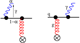
Figure 1: Direct photons production in the target rest frame. The photon can be also radiated before the quark hits the target. Both diagrams are important. The dipole cross-section appears since the quark is displaced in impact parameter plane after radiation of photon. The anti-quark enters after taking the complex conjugate of the amplitude, which is not shown here.

The hadronic cross section can be obtained by a convolution of the partonic cross section Eq. (1) with a proton structure function $F_{2}^{p}(x,Q)$ amir2 ,

$$\frac{d\sigma^{\gamma}(pt\to\gamma X)}{dx_{F}d^{2}\vec{p}_{T}d^{2}\vec{b}}=F_{2}^{p}\otimes\frac{d\sigma^{\gamma}(qt\to\gamma X)}{d(ln\alpha)d^{2}\vec{p}_{T}d^{2}\vec{b}},$$ (6)

where $x_{F}$ denotes the Feynman variable. We take the parametrization for the proton structure function given in Ref. ps .

We have recently shown that in this framework one can obtain a good description of the cross section for prompt photon production data for proton-proton (pp) collisions at RHIC and Tevatron energies amir2 . Notice also that in contrast to the parton model, in this approach neither K-factor (NLO corrections), nor higher twist corrections are to be added. No quark-to-photon fragmentation function is needed either. Indeed, the phenomenological dipole cross section fitted to DIS data incorporates all perturbative and non-perturbative radiation contributions. Predictions for the LHC in the same framework are given in Ref. us-3 . Comparison with the predictions of other approaches at the LHC can be found in Ref. lhc-hic .

III Colour dipole orientation

A colorless $\bar{q}q$ dipole is able to interact only due to the difference between the impact parameters of $q$ and $\bar{q}$ relative to the scattering center. If $\vec{s}$ is the impact parameter of the center of gravity of the dipole, and $\vec{r}$ is the transverse separation of the $q$ and $\bar{q}$, then the azimuthal angle of the radiated photons transverse momentum at a given impact parameter $\vec{s}$ correlates with the direction of $\vec{s}$. In terms of the partial elastic amplitude $f^{N}_{q\bar{q}}(\vec{s},\vec{r})$, it means that the vectors $\vec{r}$ and $\vec{s}$ are correlated.

One can see this in a simple example of a dipole interacting with a quark in Born approximation. The partial elastic amplitude reads,

$${\rm Im}f^{q}_{\bar{q}q}(\vec{s},\vec{r}) = \frac{2\alpha_{s}^{2}}{9\pi^{2}}\int\frac{d^{2}q\,d^{2}q^{\prime}}{(q^{2}+\mu^{2})(q^{\prime 2}+\mu^{2})}\,$$

$$\times \left[e^{i\vec{q}\cdot(\vec{s}+\vec{r}/2)}-e^{i\vec{q}\cdot(\vec{s}-\vec{r}/2)}\right]$$

$$\times \left[e^{i\vec{q}^{\,\prime}\cdot(\vec{s}+\vec{r}/2)}-e^{i\vec{q}^{\,\prime}\cdot(\vec{s}-\vec{r}/2)}\right]$$

$$= \frac{8\alpha_{s}^{2}}{9}\left[K_{0}\left(\mu\left|\vec{s}+\frac{\vec{r}}{2}\right|\right)-K_{0}\left(\mu\left|\vec{s}-\frac{\vec{r}}{2}\right|\right)\right]^{2},$$

where we introduced an effective gluon mass $\mu$ to take into account some nonperturbative effects. It is obvious from the above expression that the partial elastic dipole amplitude exposes a correlation between $\vec{r}$ and $\vec{s}$, and the amplitude vanishes when $\vec{s}\cdot\vec{r}=0$. In the above expression we assumed for the sake of simplicity that $q$ and $\bar{q}$ have equal longitudinal momenta, i.e. they are equally distant from the dipole center of gravity. The general case of unequal sharing of the dipole momentum will be considered later.

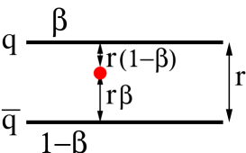
Figure 2: The relative distance of $q$ and $\bar{q}$ from the center of gravity of $q\bar{q}$ dipole varies with the fractional light-cone momenta $\beta$.

The Born amplitude is unrealistic, since it leads to an energy independent dipole cross section $\sigma_{\bar{q}q}(r,x)$. This dipole cross section has been well probed by measurements of the proton structure function at small Bjorken $x$ at HERA, and was found to rise towards small $x$, with an $x$ dependent steepness.

The dipole elastic amplitude $f^{N}_{q\bar{q}}$ of a $\bar{q}q$ dipole colliding with a proton at impact parameter $\vec{s}$ is given by us-1

$${\rm Im}f^{N}_{\bar{q}q}(\vec{s},\vec{r},\beta)=\frac{1}{12\pi}\int\frac{d^{2}q\,d^{2}q^{\prime}}{q^{2}\,q^{\prime 2}}\,\alpha_{s}\,{\cal F}(x,\vec{q},\vec{q}^{\,\prime})e^{i\vec{s}\cdot(\vec{q}-\vec{q}^{\,\prime})}$$ (8)

$$\times \left(e^{-i\vec{q}\cdot\vec{r}\beta}-e^{i\vec{q}\cdot\vec{r}(1-\beta)}\right)\,\left(e^{i\vec{q}^{\prime}\cdot\vec{r}\beta}-e^{-i\vec{q}^{\prime}\cdot\vec{r}(1-\beta)}\right)\,\,.$$

where we defined $\alpha_{s}=\sqrt{\alpha_{s}(q^{2})\alpha_{s}(q^{\prime 2})}$ and $\mathcal{F}(x,\vec{q},\vec{q}^{\,\prime})$ is the generalized unintegrated gluon density (see below). The $x$ dependence is implicit in the above expression. The fractional light-cone momenta of the quark and antiquark are denoted by $\beta$ and $1-\beta$, respectively. It is obvious that the center of gravity of $q\bar{q}$ is closer to the fastest $q$ or $\bar{q}$, see Fig. (2). The radiated photon takes away a fraction $\alpha$ of the quark momentum, see Fig. (1). Therefore, for photon production, we have

$$\beta=\frac{1}{2-\alpha}.$$ (9)

Integrating over the vector $\vec{s}$ one can recover the dipole cross section $\sigma^{N}_{q\bar{q}}(r,x)$.

$$\sigma^{N}_{q\bar{q}}(r,x) = 2\int d^{2}\vec{s}~{}\text{Im}f^{N}_{q\bar{q}}(\vec{s},\vec{r},\beta)$$ (10)

$$= \frac{4\pi}{3}\int\frac{d^{2}q}{q^{4}}(1-e^{-i\vec{q}.\vec{r}})\alpha_{s}(q^{2})\mathcal{F}(x,q).\$$

It is important to notice that the expression Eq. (8) also goes beyond the usual assumption that the dipole cross section is independent of the light-cone momentum sharing $\beta$. Although, the partial amplitude Eq. (8) does depend on $\beta$, this dependence disappears after integration over impact parameter $\vec{s}$ as shown in Eq. (10).

The generalized unintegrated gluon density $\mathcal{F}(x,\vec{q},\vec{q}^{\,\prime})$ is related to the diagonal one by

$$\mathcal{F}(x,\vec{q},\vec{q}^{\,\prime}=\vec{q})=\mathcal{F}(x,q).$$ (11)

The generalized unintegrated gluon density in Born approximation takes the form,

$${\cal F}(x,\vec{q},\vec{q}^{\,\prime}) \Rightarrow {\cal F}_{Born}(\vec{q},\vec{q}^{\,\prime})$$ (12)

$$= \frac{4\alpha_{s}}{\pi}\left[F_{N}(\vec{q}-\vec{q}^{\,\prime})-F_{N}^{(2q)}(\vec{q},\vec{q}^{\,\prime})\right],$$

where $F_{N}(k)=\langle\Psi_{N}|\exp(i\vec{k}\cdot\vec{\rho}_{1})|\Psi_{N}\rangle$ is the nucleon form factor, and $F_{N}^{(2q)}(\vec{q},\vec{q}^{\,\prime})=\langle\Psi_{N}|\exp[i\vec{q}\cdot\vec{\rho}_{1}-i\vec{q}^{\,\prime}\cdot\vec{\rho}_{2}]|\Psi_{N}\rangle$ is the so called two-quark nucleon form factor which can be calculated using the three valence quark nucleon wave function $\Psi_{N}(\vec{\rho}_{1},\vec{\rho}_{2},\vec{\rho}_{3})$.

Figure 3: The partial elastic amplitude $\text{Im}f^{N}_{q\bar{q}}$ (mb) of the $\bar{q}q$ dipole on a proton at impact parameter $s$ as a function of dipole size $r$ and angle $\delta$ between $\vec{s}$ and $\vec{r}$ for two values of $\alpha=0,1$. We use a fixed value of $x=0.01$ for all plots.

For the dipole cross section we rely on the popular saturated shape kst fitted to HERA data for $F_{2}^{p}(x,Q^{2})$. Assuming no correlation between the momenta $\vec{q}$ and $\vec{q}^{\,\prime}$ inside the Pomeron aside from the Pomeron-proton form factor, we arrive at the following form of ${\cal F}(x,\vec{q},\vec{q}^{\,\prime})$ us-1 ,

$${\cal F}(x,\vec{q},\vec{q}^{\,\prime}) = \frac{3\,\sigma_{0}}{16\,\pi^{2}\,\alpha_{s}}\ q^{2}\,q^{\prime 2}\,R_{0}^{2}(x)$$ (13)

$$\times {\rm exp}\Bigl{[}-{1\over 8}\,R_{0}^{2}(x)\,(q^{2}+q^{\prime 2})\Bigr{]}$$

$$\times {\rm exp}\bigl{[}-R_{N}^{2}(\vec{q}-\vec{q}^{\,\prime})^{2}/2\bigr{]}\,,$$

where $\sigma_{0}=23.03$ mb, $R_{0}(x)=0.4\,\mbox{fm}\times(x/x_{0})^{0.144}$ with $x_{0}=3.04\times 10^{-4}$ kst . We assume here that the Pomeron-proton form factor has the Gaussian form, $F^{p}_{\bf I\!P}(k_{T}^{2})=\exp(-k_{T}^{2}R_{N}^{2}/2)$, so the slope of the $pp$ elastic differential cross section is $B^{pp}_{el}=2R_{N}^{2}+2\alpha^{\prime}_{\bf I\!P}\ln(s/s_{0})$, where $\alpha^{\prime}_{\bf I\!P}\approx 0.25\,\mbox{GeV}^{-2}$ is the slope of the Pomeron trajectory, $s_{0}=1\,\mbox{GeV}^{2}$. $R_{N}^{2}\approx\langle r_{ch}^{2}\rangle/3$ is the part of the slope of elastic cross section related to the Pomeron-proton form factor and $\langle r_{ch}^{2}\rangle$ is the mean-square charge radius of the proton.

Unfortunately, it is not possible to uniquely determine the unintegrated gluon density function from the available data. Nevertheless, the proposed form Eq. (13) seems to be a natural generalization which preserves the saturation properties of the diagonal part us-1 .

With this unintegrated gluon density the partial amplitude Eq. (8) can be calculated explicitly,

$${\rm Im}f^{N}_{\bar{q}q}(\vec{s},\vec{r},x,\beta)=\frac{\sigma_{0}}{8\pi B_{el}}\,\Biggl{\{}\exp\left[-\frac{[\vec{s}+\vec{r}(1-\beta)]^{2}}{2B_{el}}\right]+\exp\left[-\frac{(\vec{s}-\vec{r}\beta)^{2}}{2B_{el}}\right]-2\exp\Biggl{[}-\frac{r^{2}}{R_{0}^{2}}-\frac{[\vec{s}+(1/2-\beta)\vec{r}]^{2}}{2B_{el}}\Biggr{]}\Biggr{\}},$$ (14)

where $B_{el}(x)=R_{N}^{2}+R_{0}^{2}(x)/8$.

In Fig. (3) we show the partial dipole amplitude $f^{N}_{q\bar{q}}(\vec{s},\vec{r})$ as a function of the dipole size $r$ and the angle $\delta$ between $\vec{s}$ and $\vec{r}$, at various fixed values of $s$, for two values of $\alpha=0,1$. One can see that for very small dipole sizes $r$ the dipole orientation is not important. For very large dipole sizes $r$ compared to the impact parameter $s$ or very small values of $s$ the dipole orientation is also not present. It is important to note that the generic feature of the partial dipole amplitude, e. g. its maximum and minimum pattern, changes with $\alpha$. However, it is not obvious a priori how the convolution with the proton structure function Eq. (6), which leads to a sum over all different configurations of $\alpha$ and on top of that the convolution between the partial dipole amplitude and the nuclear profile Eq. (II), which leads to a even more complicated angle mixing, gives rise to a final azimuthal asymmetry.

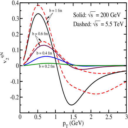
Figure 4: The anisotropy parameter $v_{2}^{qN}(b,p,\alpha)$ as function of $p_{T}$ calculated at $\alpha=1$ for different impact parameters $b$ and energies: $\sqrt{s}=200\,\mbox{GeV}$ (solid, $b=0.2,\ 0.4,\ 0.6,\ 1\,\mbox{fm}$), and $\sqrt{s}=5500\,\mbox{GeV}$ (dashed, $b=0.6,\ 1\,\mbox{fm}$). The plot is taken from Ref. us-1 .

IV Azimuthal asymmetry

The main source of azimuthal asymmetry in the amplitude (II) is the interplay between multiple rescattering and the shape of the physical system. The key function which describes the effect of multiple interactions is the eikonal exponential in Eq. (II), while the information about the shape of the system is incorporated through a convolution of the impact parameter dependent partial elastic amplitude and the nuclear thickness function. Notice that the initial space-time asymmetry gets translated into a momentum space anisotropy by the double Fourier transform in Eq. (1).

The azimuthal asymmetry of prompt photon production, resulting from parton-nucleus (qt) or proton-nucleus (pt) collisions for $t=N,A$, is defined as the second order Fourier coefficients in a Fourier expansion of the azimuthal dependence of a single-particle spectra Eq. (1) around the beam direction,

$$v_{2}^{q(p)t}(p_{T},b,\alpha)=\frac{\int_{-\pi}^{\pi}d\phi\cos(2\phi)\frac{d\sigma^{\gamma}(q(p)t\to\gamma X)}{d(ln\alpha)d^{2}\vec{p}_{T}d^{2}\vec{b}}}{\int_{-\pi}^{\pi}d\phi\frac{d\sigma^{\gamma}(q(p)t\to\gamma X)}{d(ln\alpha)d^{2}\vec{p}_{T}d^{2}\vec{b}}},$$ (15)

where the angle $\phi$ is defined with respect to the reaction plane. In the same fashion, the azimuthal asymmetry of photon yield from collisions of two nucleus A₁ and A₂ at impact parameter $B$ is defined as

$$v_{2}^{A_{1}A_{2}}(B,p_{T}) = \frac{\int_{-\pi}^{\pi}d\phi\cos(2\phi)~{}\mathcal{G}_{N}}{\int_{-\pi}^{\pi}d\phi~{}\mathcal{G}_{D}};$$

$$\mathcal{G}_{N} = \int d^{2}\vec{b}\cos(2\Theta_{1})\frac{d\sigma^{\gamma}(pA_{1}\to\gamma X)}{dx_{F}d^{2}\vec{p}_{T}d^{2}\vec{b}_{1}}T_{A_{2}}(\vec{b}_{2})$$

$$+ \int d^{2}\vec{b}\cos(2\Theta_{2})\frac{d\sigma^{\gamma}(pA_{2}\to\gamma X)}{dx_{F}d^{2}\vec{p}_{T}d^{2}\vec{b}_{2}}T_{A_{1}}(\vec{b}_{1});$$

$$\mathcal{G}_{D} = \int d^{2}\vec{b}\frac{d\sigma^{\gamma}(pA_{1}\to\gamma X)}{dx_{F}d^{2}\vec{p}_{T}d^{2}\vec{b}_{1}}T_{A_{2}}(\vec{b}_{2})$$ (16)

$$+ \int d^{2}\vec{b}\frac{d\sigma^{\gamma}(pA_{2}\to\gamma X)}{dx_{F}d^{2}\vec{p}_{T}d^{2}\vec{b}_{2}}T_{A_{1}}(\vec{b}_{1}),\$$

where we used the notation $\vec{b}_{2}=\vec{b}+\vec{B}$, $\vec{b}_{1}=\vec{b}$ ($\vec{b}$ is the impact parameter of the p$A_{1}$ collision) and the angle $\Theta_{1}$ ($\Theta_{2}$) is the angle between the vectors $\vec{b}_{1}$( $\vec{b}_{2}$) and $\vec{B}$, respectively. The medium modification of nucleon structure functions in our interested range of $p_{T}$ is less than $20\%$ and is ignored in the above expression.

The only external input in our approach is the nuclear profile. First, we take a popular Woods-Saxon (WS) profile, with a nuclear radius $R_{A}=6.5$ fm and a surface thickness $\xi=0.54$ fm, for Pb+Pb collisions ws .

In Fig. 4, we show examples of azimuthal anisotropy from quark-nucleon collisions radiating a photon $v_{2}^{qN}(b,p,\alpha)$, with $\alpha=1$ and at different impact parameters and energies. The results show that the anisotropy of the dipole interaction rises with impact parameter, reaching rather large values. As function of the transverse momentum of the radiated photons, $v_{2}^{qN}(b,p,\alpha)$ vanishes at large $p_{T}$. Such a behavior could be anticipated, since the interaction of vanishingly small dipoles responsible for large $p$ is not sensitive to the dipole orientation.

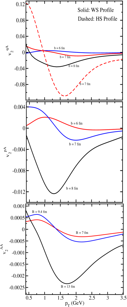
Figure 5: The impact parameter dependence of prompt photon azimuthal asymmetry, for q+Pb (at $\alpha=1$), p+Pb and Pb+Pb collisions for RHIC energy at midrapidities, with the Woods-Saxon (WS) nuclear profile. As example, we have also shown in the first panel, the prompt photon elliptic anisotropy from q+pb collisions for the hard sphere (HS) nuclear profile. The plot is taken from Ref. us-2 .

In Fig. (5), we show the calculated values of $v_{2}^{q(p)A}$ defined in Eq. (15), for fixed $\alpha=1$, at various q(p)A collision impact parameters $b$ for the RHIC energy $\sqrt{\mathbb{s}}=200$ GeV at midrapidities. If the nuclear profile function was constant, then the convolution between the nuclear profile and the dipole orientation, defined in Eq. (II), would be trivial, and $v_{2}^{qA}$ becomes then identically zero. Therefore, the main source of azimuthal anisotropy is not present for central collisions where the correlation between nuclear profile and dipole orientation is minimal. This can be seen in Fig. (5), where a pronounced elliptic anisotropy is observed for collisions with impact parameters close to the nuclear radius $R_{A}$, where the nuclear profile undergoes rapid changes. Therefore, the important parameter which controls the elliptic asymmetry in this mechanism is $|b-R_{A}|$ us-1 .

It is important to notice that $v^{qA}_{2}$ is suppressed an order of magnitude compared to $v^{qN}_{2}$. At first glance this might look strange, since the quark interacts with nucleons anyway. However, a quark propagating through a nucleus interacts with different nucleons located at different azimuthal angles relative to the quark trajectory. Their contributions to $v_{2}^{qA}$ tend to cancel each other, restoring the azimuthal symmetry. Such cancellation would be exact if the nuclear profile function $T_{A}(b)$ were constant. We have a nonzero, but small $v_{2}^{qA}$ only due to the variation of $T_{A}$ with $b$. Going from $q(p)A$ to $AA$ collisions, see Fig. (5), the elliptic asymmetry is further reduced. The main reason is that the integrand in Eq. (16) gets contributions only from semi-peripheral pA collisions where our mechanism is at work, and most of the integral over $\vec{b}$ does not contribute. This significantly dilutes the signal.

V On the sign of $\mathbb{v_{2}}$

In Fig. (3), we showed that the general behaviour of dipole amplitude orientation, e.g. its maximum and minimum pattern changes with the parameter $\beta$ which defines the relative position of the center of gravity of the dipole from the $q$ and $\bar{q}$, see Fig. (2). Here, we take a heuristic approach, and explore a possible link between the peculiar behaviour of $v_{2}$ shown in Fig. (5) with the dipole orientation introduced in Eq. (8).

Let us assume for sake of argument that the parameter $\beta$ is independent of $\alpha$ and assume that $q$ and $\bar{q}$ have equal longitudinal momenta namely $\beta=1/2$. This corresponds to a particular configuration in which the dipole amplitude is symmetric under $\vec{r}\to-\vec{r}$, see Fig. (3). In principle, this configuration is kinematically less probable for direct photon production (in contrast to DIS) since it corresponds to $\alpha=0$ via Eq. (9). Notice that although we take a fixed $\beta=1/2$ in the dipole amplitude Eq. (8), the LC distribution of the projectile quark $\gamma q$ fluctuation Eq. (2) still depends on $\alpha$ and also the transverse dipole size is $\alpha\vec{r}$ and varies with $\alpha$, see Eq. (1).

We repeat the computation of the azimuthal asymmetry $v_{2}$ of prompt photons in the same way as discussed in the previous section. For example, in Fig. (6), we show the anisotropy asymmetry $v_{2}^{qN}$ and $v_{2}^{qA}$ at $\alpha=1$ for various impact parameters as in Figs. (4,5). Comparing with the results presented in the previous section, it is seen that although the order of magnitude of $v_{2}$ is the same in both cases, now the sign of $v_{2}$ does not change at higher $p_{T}$ and remains positive. This indicates that the sign of $v_{2}$ in this mechanism is related to the dipole orientation via the parameter $\beta$.

Notice also that the sign behaviour of the prompt photon $v_{2}$ for $AA$ collisions at higher $p_{T}$ is also present for both $qN$ and $qA$ collisions.

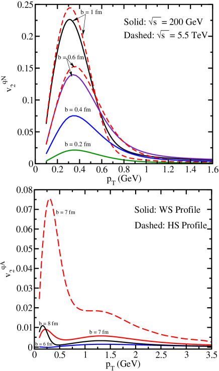
Figure 6: Upper panel: The anisotropy parameter $v_{2}^{qN}(b,p,\alpha)$ as function of $p_{T}$ for different impact parameters $b$ for RHIC and LHC energies. Down panel: The anisotropy parameter $v_{2}^{qA}(b,p,\alpha)$ as function of $p_{T}$ for various impact parameter $b$ for RHIC energy at midrapidity. Similar to Fig. (5) we show the results for both the WS and the HS nuclear profiles. In both plots the results calculated at a fixed $\beta=1/2$ in the dipole amplitude and $\alpha=1$.

VI Concluding remarks

The azimuthal elliptic asymmetry $v_{2}$ observed in heavy ion collisions is usually associated with properties of the medium created in the final state. We introduced a novel mechanism which relates this azimuthal asymmetry to the colour dipole orientation. To this end, we proposed a model generalizing the unintegrated gluon density fitted to data for the proton structure function to an off-diagonal unintegrated gluon distribution.

We showed that the azimuthal asymmetry $v_{2}$ of prompt photons changes sign and becomes negative for peripheral collisions. Although this behaviour seems to be robust for the considered range of $p_{T}$, there is some uncertainty on the magnitude of the $v2$ coming from this mechanism. The shape of the tail of nuclear profile is important in this mechanism, since it significantly affects the results. To highlight this point, in Figs. (5,6), we have also shown the azimuthal asymmetry from quark-nucleus collisions $v_{2}^{qA}$ for the hard sphere (HS) nuclear profile. By comparing with the results from the WS nuclear profile for the same setting, one may conclude that the maximum uncertainty in this mechanism can be as big as an order of magnitude. Unfortunately the tail of all available nuclear profile parametrizations is less reliable and obtained by a simple extrapolation ws . This is also due to the fact that the neutron distribution, which may be more important on the periphery, cannot be properly accounted for by electron scattering data. Another source of uncertainty in this approach is due to the fact that the off-diagonal part of the unintegrated gluon density cannot be uniquely defined from the current experimental data.

In order to see if this mechanism is relevant to heavy ion collisions, it would be of great interest to calculate the azimuthal asymmetry for gluon radiation and hadron production at RHIC. This mechanism might also contribute to the azimuthal asymmetry in DIS and in the production of dileptons. We plan to report on some of these problems in the near future.

- (1) PHENIX Collaboration, arXiv:0705.1711.
- (2) PHENIX Collaboration, Phys. Rev .Lett. 96, 032302 (2006).
- (3) B. Z. Kopeliovich, H. J. Pirner, A. H. Rezaeian, Ivan Schmidt, Phys. Rev. D77, 034011 (2008)[arXiv:0711.3010].
- (4) B. Z. Kopeliovich, A. H. Rezaeian, Ivan Schmidt, arXiv:0712.2829, Accepted for publication in Nucl. Phys. A.
- (5) S. Turbide, C. Gale and R. J. Fries, Phys. Rev. Lett. 96, 032303 (2006).
- (6) S. Turbide, C. Gale, E. Frodermann, U. Heinz, Phys. Rev. C77, 024909 (2008) [arXiv:0712.0732].
- (7) R. Chatterjee, E. S. Frodermann, U. W. Heinz, D. K. Srivastava, Phys .Rev. Lett. 96, 202302 (2006).
- (8) F. M. Liu and K. Werner, arXiv:0712.3619.
- (9) K. Golec-Biernat and M. Wüsthoff, Phys. Rev. D59, 014017 (1999).
- (10) B.Z. Kopeliovich, A. Schaefer and A.V. Tarasov, Phys. Rev. C59 (1999) 1609
- (11) B. Z. Kopeliovich, A. H. Rezaeian, H. J. Pirner and Ivan Schmidt, Phys. Lett. B653, 210 (2007).
- (12) SMC Collaboration, Phys. Rev. D58, 112001 (1998).
- (13) A. H. Rezaeian, B. Z. Kopeliovich, H. J. Pirner and Ivan Schmidt, arXiv:0707.2040.
- (14) S. Abreu et al., arXiv:0711.0974.
- (15) A. Bohr and B. R. Mottelson, Nuclear Structure (Benjamin, New York, 1969); C. W. De Jager, H. De Vries, C. De Vries, Atom. Data Nucl. Data Tables 36, 496 (1987).