Transport coefficients of multi-particle collision algorithms with velocity-dependent collision rules

Abstract

Detailed calculations of the transport coefficients of a recently introduced particle-based model for fluid dynamics with a non-ideal equation of state are presented. Excluded volume interactions are modeled by means of biased stochastic multiparticle collisions which depend on the local velocities and densities. Momentum and energy are exactly conserved locally. A general scheme to derive transport coefficients for such biased, velocity dependent collision rules is developed. Analytic expressions for the self-diffusion coefficient and the shear viscosity are obtained, and very good agreement is found with numerical results at small and large mean free paths. The viscosity turns out to be proportional to the square root of temperature, as in a real gas. In addition, the theoretical framework is applied to a two-component version of the model, and expressions for the viscosity and the difference in diffusion of the two species are given.

1 Introduction

The interplay between hydrodynamic interactions and thermal fluctuations is crucial for a wide range of phenomena in biophysics and soft-matter physics. Several particle-based simulation methods such as dissipative particle dynamics [1, 2], smooth particle hydrodynamics [3], and direct simulation Monte Carlo [4, 5] have been developed for the efficient modeling of these phenomena with the motivation to coarse-grain out irrelevant atomistic details while correctly incorporating the essential physics. One particular method was introduced by Malevanets and Kapral in 1999 [6, 7] and is often called stochastic rotation dynamics (SRD) [8, 9, 10, 11, 12] or multi-particle collision dynamics (MPC) [13, 14, 15, 16]. The method is based on so-called fluid particles with continuous positions and velocities which follow a simple, artificial dynamics and undergo efficient multi-particle collisions. The original SRD algorithm models a fluid with an ideal gas equation of state. Recently, the collision rules of the original algorithm have been generalized to model excluded-volume effects, allowing for a more realistic modeling of dense gases and immiscible binary fluids [17, 18]. These new multi-particle collision rules depend on local densities and velocities. The new models can be thought of as a coarse-grained multi-particle collision generalization of a hard sphere fluid since, just as for hard spheres, there is no internal energy. Their static properties such as the equation of state and the entropy density have been derived recently [17, 18], and were shown to be in excellent agreement with numerical results for the pressure, speed of sound, density fluctuations and the phase diagram. However, the dynamic properties are not yet fully understood. Some preliminary results about the transport coefficients were published previously [17, 18, 19, 20], but without derivation and without results for the viscosity at small mean free path. In this paper I present the details of how to derive expressions for the self-diffusion coefficient and the shear viscosity at small and large mean free path. For simpler, unbiased collison rules, this was done before [8, 10, 11, 21, 22]; the added difficulty here is that the collision probabilities depend on the particle velocities which leads to strong correlations. The derived formulas will be compared to numerical simulations in various limits.

The paper is structured as follows: section 2 introduces the simulation model, and in section 3 the self-diffusion coefficient is derived. In section 4 an equilibrium method to determine the kinetic part of the viscosity is used: Green-Kubo relations of the kinetic stress correlations are evaluated. Section 5 applies a non-equlibrium method to calculate the collisional contribution to the viscosity by evaluating the momentum transfer in shear flow. This non-equilibrium method is a more rigorous version of the earlier approach introduced in ref. [8] and now, in principle, can be used to obtain the shear dependence of the collisional viscosity. In section 6 the developed scheme is applied to calculate transport coefficients for a binary model and a model with a large collision rate.

2 Model

As in the original SRD algorithm, the solvent is modeled by a large number $N$ of point-like particles of mass $m_{p}$ which move in continuous space with a continuous distribution of velocities. The particle mass is set equal to one throughout this paper. The system is coarse-grained into $(L/a)^{d}$ cells of a $d$-dimensional cubic lattice of linear dimension $L$ and lattice constant $a$. The algorithm consists of individual streaming and collision steps. In the free-steaming step, the coordinates, ${\bf r}_{i}(t)$, of the solvent particles at time $t$ are updated according to ${\bf r}_{i}(t+\tau)={\bf r}_{i}(t)+\tau{\bf v}_{i}(t)$, where ${\bf v}_{i}(t)$ is the velocity of particle $i$ at time $t$ and $\tau$ is the value of the discretized time step. In order to define the collision, we introduce a second grid with sides of length $2a$ which (in $d=2$) groups four adjacent cells into one “supercell”.

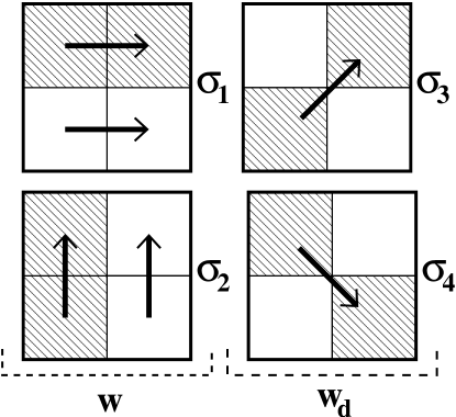
Figure 1: Schematic collision rules. Momentum is exchanged in three ways: a) horizontally along $\mbox{\boldmath$\sigma$}_{1}$, b) vertically along $\mbox{\boldmath$\sigma$}_{2}$, c) diagonally along $\mbox{\boldmath$\sigma$}_{3}$ and $\mbox{\boldmath$\sigma$}_{4}$. $w$ and $w_{d}$ denote probabilities of choosing a), b) and c), respectively. From ref. [17].

As proposed in Refs. [8, 9], a random shift of the particle coordinates before the collision step is required to ensure Galilean invariance. All particles are therefore shifted by the same random vector with components in the interval $[-a,a]$ before the collision step (Because of the supercell structure, this is a larger interval than in the conventional SRD algorithm). Particles are then shifted back by the same amount after the collision. To initiate a collision, pairs of cells in every supercell are randomly selected. As shown in fig. 1, three different choices are possible: a) horizontal (with $\mbox{\boldmath$\sigma$}_{1}=\hat{x}$), b) vertical ($\mbox{\boldmath$\sigma$}_{2}=\hat{y}$), and c) diagonal collisions (with $\mbox{\boldmath$\sigma$}_{3}=(\hat{x}+\hat{y})/\sqrt{2}$ and $\mbox{\boldmath$\sigma$}_{4}=(\hat{x}-\hat{y})/\sqrt{2}$). Note that diagonal collisions are essential to equilibrate the kinetic energies in the $x-$ and $y-$directions.

In every cell, we define the mean particle velocity,

$${\bf u}_{n}={1\over M_{n}}\,\sum_{i=1}^{M_{n}}\,{\bf v}_{i},$$ (1)

where the sum runs over all particles, $M_{n}$, in the cell with index $n$. The projection of the difference of the mean velocities of the selected cell-pairs on ${\bf\sigma}_{j}$, $\Delta u={\bf\sigma}_{j}\cdot({\bf u}_{1}-{\bf u}_{2})$, is then used to determine the probability of collision. If $\Delta u<0$, no collision will be performed. For positive $\Delta u$, a collision will occur with an acceptance probability which depends on $\Delta u$ and the number of particles in the two cells, $M_{1}$ and $M_{2}$. This rule mimics a hard-sphere collision on a coarse-grained level: For $\Delta u>0$ clouds of particles collide and exchange momenta. The following acceptance probability was introduced in ref. [17]

$$p_{A}(M_{1},M_{2},\Delta u)=\theta(\Delta u)\,\,{\rm tanh}(\Lambda)\ \ \ \ {\rm with}\ \ \ \ \Lambda=A\,\Delta u\,M_{1}M_{2},$$ (2)

where $\theta$ is the unit step function and $A$ is a parameter which allows us to tune the equation of state. The hyperbolic tangent function was chosen in (2) in order to obtain a probability which varies smoothly between 0 and 1. This paper treats the two most relevant limits for the acceptance probability: In the first one, which was proven to be thermodynamically consistent, one keeps the collision parameter $A$ small such that the $tanh$ can be replaced by its argument. In the other limit, $p_{A}$ is simply the theta function alone which is equivalent to let $A$ go to infinity. In principle, any other situation with $A<\infty$ can be handled by expanding the $tanh$; all additional terms still contain solvable integrals.

Once it is decided to perform a collision, an explicit form for the momentum transfer between the two cells is needed. The collision should conserve the total momentum and kinetic energy of the cell-pairs participating in the collision, and in analogy to the hard-sphere liquid, the collision should primarily transfer the component of the momentum which is parallel to the connecting vector $\mbox{\boldmath$\sigma$}_{j}$. This component will be called the parallel or longitudinal momentum. There are many different choices which fulfill these conditions. Since the original goal was to obtain a large speed of sound, a collision rule was selected which leads to the maximum transfer of the parallel component of the momentum and does not change the transverse momentum. The rule is quite simple; it exchanges the parallel component of the mean velocities of the two cells, which is equivalent to a “reflection” of the relative velocities,

$$v_{i}^{\|}(t+\tau)-u^{\|}=-(v_{i}^{\|}(t)-u^{\|})\,,$$ (3)

where $u^{\|}$ is the parallel component of the mean velocity of the particles of both cells. The perpendicular component remains unchanged,

$$v_{i}^{\perp}(t+\tau)=v_{i}^{\perp}(t).$$ (4)

More specifically, the rule for horizonal collisions in $\mbox{\boldmath$\sigma$}_{1}$ direction is simply

$$\tilde{v}_{i,x}=2u_{x}-v_{i,x}$$ (5)

with $\tilde{v}_{i,x}$ denotes $v_{i,x}(t+\tau)$. The y-components of the particle velocities stay the same, $\tilde{v}_{i,y}=v_{i,y}$. For the upward diagonal collision along the $\mbox{\boldmath$\sigma$}_{3}$ direction one has

$$\tilde{v}_{i,x}=u_{x}+u_{y}-v_{i,y}$$

$$\tilde{v}_{i,y}=u_{x}+u_{y}-v_{i,x}$$ (6)

It is easy to verify that these rules conserve momentum and energy in the cell pairs.

Because of $x-y$ symmetry, the probabilities for choosing cell pairs in the $x-$ and $y-$ directions (with unit vectors $\mbox{\boldmath$\sigma$}_{1}$ and $\mbox{\boldmath$\sigma$}_{2}$, see fig. 1) are equal, and will be denoted by $w$. The probability for choosing diagonal pairs ($\mbox{\boldmath$\sigma$}_{3}$ and $\mbox{\boldmath$\sigma$}_{4}$, see fig. 1) is given by $w_{d}=1-2w$. $w$ and $w_{d}$ must be chosen such that the hydrodynamic equations are isotropic and do not depend on the orientation of the underlying grid. This was done by considering the temporal evolution of the lowest moments of the velocity distribution function, or alternatively, by evaluating the isotropy of the kinetic part of the viscous stress tensor [18, 20]. Both approaches concluded that $w=1/4$ and $w_{d}=1/2$, and previous simulations show that both the speed of sound and the shear viscosity are isotropic for this choice. Note, however, that this does not guarantee that all properties of the model are isotropic. This becomes apparent at high densities or high collision frequency, $1/\tau\gg 1$, where the cubic anisotropy of the grid shows leading to inhomogeneous states with cubic symmetry [17].

3 Diffusion coefficient

The self-diffusion constant $D$ is given by a sum over the velocity-autocorrelation function (eq. (102) in [9]),

$$D=\tau\,\left.\sum_{n=0}^{\infty}\right.^{\prime}\langle v_{x}(0)\,v_{x}(n\tau)\rangle\,,$$ (7)

where the prime on the sum indicates that the $n=0$ term has the relative weight $1/2$. The particle mass is set to one throughout the paper. Assuming molecular chaos, one has

$$\langle v_{x}(0)\,v_{x}(n\tau)\rangle = k_{B}T\,g^{n}\;\;{\rm where}\;\;\;g={\langle v_{x}(0)\,v_{x}(\tau)\rangle\over k_{B}T}$$ (8)

and the sum (7) turns into a geometric series which is easily summed up to give

$$D={k_{B}T\,\tau\over 2}\,{1+g\over 1-g}\,.$$ (9)

$g$ is the velocity correlation one time step apart, which completely defines the diffusion coefficient in the molecular chaos approximation. There is four different contributions to $g$ as a result of possible horizontal, vertical, and the two diagonal collisions:

$$g=w(g_{H}+g_{V})+{w_{d}\over 2}(g_{U}+g_{D})$$ (10)

The vertical, $g_{V}$, and the horizontal contribution, $g_{H}$, occur with probability $w=1/4$, whereas the upward diagonal part, $g_{U}$ and the downward diagonal part, $g_{D}$, enter with probability $w_{d}=1/2$. The additional factor $1/2$ in front of the second bracket accounts for the fact that the two diagonal collisions are always chosen together and on average only $1/2$ of the particles in a $2a\times 2a$-super cell undergo an upward diagonal collision while the other half is subject to a downward diagonal collision. In contrast, in a horizontal (or vertical) collision operation all particles in the super-cell can in principle be involved in the collision since the super cell is divided in two double cells with horizontal (or vertical) collisions in each one. The contribution due to vertical collisions is easy to calculate, since in this case, the value of $v_{i,x}$ is unchanged in a collision, eq. (4), and $v_{i,x}(\tau)=v_{i,x}(0)$. Following eq. (8) we find

$$g_{V}={\langle v_{i,x}(0)\,v_{i,x}(\tau)\rangle\over k_{B}T}=1$$ (11)

3.1 Horizonal collisions

Consider now the horizontal contribution, $g_{H}$. We assume that there are $n$ particles in the left subcell, and $m$ particles in the right subcell of the cell pair where the collision happens. It is also assumed, that the tagged particle $i$ is contained in the left subcell. For the moment the particle numbers $n$ and $m$ are kept fixed. According to eq. (2), for small $A$, a collision occurs with the acceptance probability,

$$p_{A}=A\,n\,m\;\theta(\Delta u)\;\Delta u\,;$$ (12)

and the value of $v_{i,x}$ changes in the following way $v_{i,x}(\tau)=2u_{x}-v_{i,x}(0)$. Here, $u_{x}$ is the x-component of the mean velocity of both subcells:

$$u_{x}={1\over n+m}\sum_{j=1}^{n+m}\,v_{j,x}$$ (13)

For horizontal directions, $\Delta u$ contains only the x-components of the particle velocities:

$$\Delta u={1\over n}\sum_{j=1}^{n}\,v_{j,x}-{1\over m}\sum_{j=n+1}^{n+m}\,v_{j,x}\,.$$ (14)

.

If a collision is not accepted, which happens with probability $1-p_{A}$, the value of $v_{i,x}$ remains unchanged: $v_{i,x}(\tau)=v_{i,x}(0)$. From these considerations it follows,

$$g_{H}={1\over k_{B}T}\langle p_{A}\,v_{i,x}(2u_{x}-v_{i,x})+(1-p_{A})v_{i,x}^{2}\rangle\,.$$ (15)

The average is performed over the velocity distribution (at time $t=0$) of all involved particles and over the particle numbers in the two subcells forming a collision cell. Note that there is a non-trivial coupling between the velocity-dependent acceptance probability $p_{A}$ and the updated velocity $v_{j,x}(\tau)$. Ignoring this coupling, which amounts to the approximation $\langle p_{A}\,v_{j,x}(0)v_{j,x}(\tau)\rangle\approx\langle p_{A}\rangle\langle v_{j,x}(0)v_{j,x}(\tau)\rangle$ leads to an errorous result which is a factor of about two smaller than the correct one, even for large particle numbers $n$, $m$.

Using $\langle v_{i,x}^{2}\rangle=k_{B}T$, eq. (15) simplifies to

$$g_{H}=1+{2\over k_{B}T}\langle p_{A}\,v_{i,x}(u_{x}-v_{i,x})\rangle\,=1+{2\over k_{B}T}\langle K_{nm}\rangle_{n,m}$$ (16)

The average $\langle...\rangle_{n,m}$ denotes an average over the particle number distribution in the two subcells (which are Poisson-distributed and uncorreletad in an ideal gas). $K_{nm}$ contains the average of the velocity distribution, which is Maxwellian if molecular chaos is assumed; and it has to be split up in two parts,

$$K_{nm}={1\over 2}\left(K_{nm}^{l}+K_{nm}^{r}\right)$$ (17)

because there are two possibilities occuring with probability $1/2$, respectively : (i) the tagged particle $i$ can be in the left subcell as one of the $n$ particles there, or (ii) can be in the right subcell with a total of $m$ particles. Hence, one has

$$K_{nm}^{l} = A\,n\,m\,J_{nm}^{l}\;\;\;{\rm with}$$

$$J_{nm}^{l} = \int_{-\infty}^{+\infty}\,dv_{i,x}^{n+m}\,\theta\left(\Delta u\right)\,\Delta u\,v_{1,x}(u_{x}-v_{1,x})\,\prod_{i=1}^{n+m}\,f_{0}(v_{i,x})\,.$$ (18)

$f_{0}(v_{i,x})$ is the Maxwell-Boltzmann distribution,

$$f_{0}(v_{i,x})=\Gamma\,{\rm exp}\left(-{v_{i,x}^{2}\over 2k_{B}T}\right)\,,\;\;\;{\rm with}\;\;\Gamma={1\over\sqrt{2\pi k_{B}T}}\,.$$ (19)

Assuming the tagged particle to be in the left subcell in the definition of $J_{nm}^{l}$ means also that $n>0$ in the expression for $J_{nm}^{l}$. For the same reason, $m$ must be larger than zero in expressions for $J_{nm}^{r}$.

Because of the $\theta$-function the direct evaluation of the $(n+m)$-dimensional integral becomes very tedious for large $n,m$. Therefore, we express the $\theta$-function by means of the $\delta$-function,

$$\theta(\Delta u)=\int_{0}^{\infty}\,\delta(\Delta u-c)\,dc$$ (20)

which allows us to use the integral-representation of the $\delta$-function,

$$\delta(\Delta u-c)=\int_{-\infty}^{+\infty}\,{\rm exp}(ik(\Delta u-c))\,{dk\over 2\pi}$$ (21)

Even though this transformation leads to two more integrations it enables a straightforward calculation of $J_{nm}^{l}$ for arbitrary $n$ and $m$. It involves only simple integrals of type $\int_{0}^{\infty}x^{n}\,exp(-x^{2})$ with $n=0,1,2,3$. The integral to be solved is:

$$J_{nm}^{l}=\Gamma^{n+m}\int_{0}^{\infty}\,dc\,\int_{-\infty}^{\infty}\,{dk\over 2\pi}\int_{-\infty}^{+\infty}\,dv_{i,x}^{n+m}$$ (22)

$$\times {\rm exp}\left[ik\left({1\over n}\sum_{j=1}^{n}\,v_{j,x}-{1\over m}\sum_{j=n+1}^{n+m}\,v_{j,x}-c\right)-{1\over 2k_{B}T}(v_{1,x}^{2}+...+v_{n+m,x}^{2})\right]$$

$$\times v_{1,x}\,\left({1\over n}\sum_{j=1}^{n}\,v_{j,x}-{1\over m}\sum_{j=n+1}^{n+m}v_{j,x}\right)\,\left({1\over n+m}\sum_{j=1}^{n+m}\,v_{j,x}-v_{1,x}\right)\,.$$

First, the argument of the exponential has to be transformed into a sum of squares in order to decouple the velocities and to enable integrating over them. This is achieved by the transformations for the velocities in the left subcell:

$$w_{i}=v_{i,x}-{k_{B}Tik\over n}\;\;{\rm for}\;i=1...n$$ (23)

and for the ones in the right subcell,

$$w_{i}=v_{i,x}+{k_{B}Tik\over m}\;\;{\rm for}\;i=n+1...n+m\,.$$ (24)

Expressing eq. (22) in the new variables $w_{i}$ gives:

$$J_{nm}^{l} = \Gamma^{n+m}\int_{0}^{\infty}\,dc\,\int_{-\infty}^{\infty}\,{dk\over 2\pi}\int_{-\infty}^{+\infty}\,dw_{i}^{n+m}$$ (25)

$$\times {\rm exp}\left(-ikc-{k_{B}T\gamma k^{2}\over 2}\right)\,{\rm exp}\left({1\over 2k_{B}T}\left[w_{1}^{2}+w_{2}^{2}+...+w_{n+m}^{2}\right]\right)$$

$$\left({w_{1}+w_{2}+...+w_{n}\over n}-{w_{n+1}+w_{n+2}+...+w_{n+m}\over m}+k_{B}Tik\gamma\right)$$

$$\left(w_{1}+{k_{B}Tik\over n}\right)\left({w_{1}+w_{2}+...+w_{n+m}\over n+m}-w_{1}-{k_{B}Tik\over n}\right)$$

with $\gamma=(1/n)+(1/m)$. The integration over the $w_{i}$ is straightforward and yields

$$J_{nm}^{l} = \Gamma^{n+m}\int_{0}^{\infty}\,dc\,\int_{-\infty}^{\infty}\,{dk\over 2\pi}$$

$$\times{\rm exp}\left(-ikc-{k_{B}T\gamma k^{2}\over 2}\right)\left[{(k_{B}T)^{3}ik^{3}\gamma\over n^{2}}+S(k_{B}T)^{2}ik\right]$$

$$S = -{2\over n^{2}}+\gamma\left({1\over n+m}-1\right)$$ (26)

The remaining integral over $h$ and $k$ is done easily using similiar transformations. The final result is:

$$J_{nm}^{l}=-{(k_{B}T)^{3/2}\over\sqrt{2\pi\gamma}}\left[{1\over n^{2}}+\left({1\over n}+{1\over m}\right)\left(1-{1\over n+m}\right)\right]$$

which is always negative.

The quantity $J_{nm}^{r}$ is given by an expression almost identical to eq. (3.1), one merely has to replace $v_{1,x}$ by $v_{n+1,x}$ at the two positions where $v_{1,x}$ appears isolated. This changes the index of the tagged particle from $1$ to $n+1$, meaning that this particle is not in the left subcell but in the right one. One finds $J_{nm}^{r}=J_{mn}^{l}$ leading to an expression for $J_{nm}$ which is symmetric in $n$ and $m$:

$$K_{nm}={Anm\over 2}(J_{nm}^{l}+J_{nm}^{r})=-{A(k_{B}T)^{3/2}\over\sqrt{2\pi\gamma}}\left[{n^{2}+m^{2}\over 2nm}+n+m-1\right]$$

Using eqs. (16-18) $g_{H}$ is calculated. In an ideal gas, $K_{nm}$ has to be averaged over the poisson-distributed particle numbers in the subcells, $n$ and $m$. In the current model with a non-ideal equation of state, particle number fluctuations are supressed compared to an ideal gas. Therefore, we will neglect these fluctuations completely for the moment, and replace $n$ and $m$ by the mean number of particles in a subcell $M=\langle n\rangle=\langle m\rangle$. This leads to the final result

$$g_{H}=1-2A\sqrt{{k_{B}T\over\pi}}M^{3/2}$$ (27)

3.2 Diagonal collisions

Here, the upward diagonal collision (along $\mbox{\boldmath$\sigma$}_{3}$ in fig. 1) is considered first. In this case, the velocity difference, $\Delta u$, depends on both the x- and the y-component of the particle velocities,

$$\Delta u=\mbox{\boldmath$\sigma$}_{3}\cdot\left({\bf u}_{1}-{\bf u}_{2}\right)={1\over\sqrt{2}}\left(u_{1,x}-u_{2,x}+u_{1,y}-u_{2,y}\right)$$ (28)

with the normal vector of the diagonal collision direction, $\mbox{\boldmath$\sigma$}_{3}=(1,1)/\sqrt{2}$, leading to a more involved calculation of $g_{U}$. Furthermore, both components of the velocities change in a collision, but only the change of the x-component is needed:

$$v_{i,x}(\tau)=u_{x}+u_{y}-v_{i,y}$$

This change occurs with probability $p_{A}$, see eq. (12), but with $\Delta u$ given in eq. (28). It follows

$$g_{U}={1\over k_{B}T}\langle p_{A}\,v_{i,x}(u_{x}+u_{y}-v_{i,y})+(1-p_{A})v_{i,x}^{2}\rangle\,.$$ (29)

The average must be done over the velocity distribution (at time $t=0$) of all involved particles and over the particle number in the two subcells forming a collision or double-cell. Because of $\langle v_{i,x}^{2}\rangle=k_{B}T$ we can write

$$g_{U}=1+{1\over k_{B}T}\langle R_{nm}-L_{nm}\rangle_{n,m}$$ (30)

with the abbrevations

$$R_{nm} = \langle p_{A}\,v_{i,x}(u_{x}+u_{y}-v_{i,y})\rangle_{T}$$ (31)

$$L_{nm} = \langle p_{A}\,v^{2}_{i,x}\rangle_{T}$$ (32)

The subscript $T$ means that only the thermal average is taken; the particle numbers $n$ and $m$ of the subcells are kept fixed in this average.

We consider again the two equivalent situations that the tagged particle is in the left subcell with a total of $n$ cells denoted by the superindex $l$, or in the right cell, described by the superindex $r$. Both possibilities occur with equal probability $1/2$ and we have

$$R_{nm} = {1\over 2}\left(R_{nm}^{l}+R_{nm}^{r}\right)$$

$$L_{nm} = {1\over 2}\left(L_{nm}^{l}+L_{nm}^{r}\right)$$ (33)

Other abbreviations are introduced as $R_{nm}=Anm\,F_{nm}$, and $L_{nm}=Anm\,I_{nm}$. This time the y-component of the velocities shows up in the calculations, leading to a $2n+2m$-dimensional integral for $F_{nm}^{l}$. We again adopt the trick to express the $\theta$-function in the acceptance probability $p_{A}$ by means of an integral over the $\delta$-function and use the integral representation of $\delta(x)$, which yields the following integral:

$$F_{nm}^{l} = \Gamma^{n+m}\int_{0}^{\infty}\,dc\,\int_{-\infty}^{\infty}\,{dk\over 2\pi}\int_{-\infty}^{+\infty}\,dv_{i,x}^{n+m}\,\int_{-\infty}^{+\infty}\,dv_{i,y}^{n+m}$$ (34)

$$\times {\rm exp}\left\{ik\left({1\over\sqrt{2}}\left[{1\over n}\sum_{j=1}^{n}\,(v_{j,x}+v_{j,y})-{1\over m}\sum_{j=n+1}^{n+m}\,(v_{j,x}+v_{j,y})\right]-h\right)\right\}$$

$$\times {\rm exp}\left\{-{1\over 2k_{B}T}\left(v_{1,x}^{2}+...+v_{n+m,x}^{2}+v_{1,y}^{2}+...+v_{n+m,y}^{2}\right)\right\}$$

$$\times {v_{1,x}\over\sqrt{2}}\,\left({1\over n}\sum_{j=1}^{n}\,(v_{j,x}+v_{j,y})-{1\over m}\sum_{j=n+1}^{n+m}(v_{j,x}+v_{j,y})\right)$$

$$\times \left({1\over n+m}\sum_{j=1}^{n+m}\,(v_{j,x}+v_{j,y})-v_{1,y}\right)\,.$$

This integral is solved straightforwardly in a very similar fashion to the one in eq. (22). The final result is

$$F_{nm}^{l}={(k_{B}T)^{3/2}\over\sqrt{2\pi\gamma}}\left[{1\over nm}-{1\over 2n^{2}}\right]$$ (35)

A similar calculation leads to

$$I_{nm}^{l}={(k_{B}T)^{3/2}\over\sqrt{2\pi\gamma}}\left[\gamma+{1\over 2n^{2}}\right]$$ (36)

Again, we observe the symmetry that the quantities with upper index $r$ follow from the ones with index $l$ by simply interchanging $n$ and $m$ in the obtained expressions: $F_{nm}^{r}=F_{mn}^{l}$, $I_{nm}^{r}=I_{mn}^{l}$. Inserting these results into eq. (30) and neglecting particle number fluctuations gives

$$g_{U}=1-A\sqrt{{k_{B}T\over\pi}}M^{3/2}$$ (37)

The evaluation of the downward diagonal contribution was done in a similar way, and for symmetry reasons one finds $g_{D}=g_{U}$. According to eqs. (27), (37) and (9), (10) the diffusion coefficient follows in the limit of small collision parameter $A$ as

$$D=k_{B}T\,\tau\left({1\over A}\,\sqrt{\pi\over k_{B}T}\;M^{-3/2}-{1\over 2}\right)\,,$$ (38)

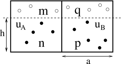
Figure 2: A double cell consisting of two subcells for horizonal collisions along the $\mbox{\boldmath$\sigma$}_{1}$ direction defined in fig. 1. $u_{A}$ is the horizontal component of the mean velocity of the $n+m=N_{A}$ particles in the left subcell. The horizontal component of the $p+q=N_{B}$ particles in the right subcell is given by $u_{B}$.

which is in good agreement with simulation data, see fig. 2. It is interesting to note, that the contributions to $D$ from the vertical and horizontal collisions together, $(g_{H}+g_{V})/4$, are exactly equal to the ones from the diagonal ones, $(g_{U}+g_{D})/4$, which is a sign of the correct isotropic choice of the probabilities $w$ and $w_{d}$.

3.3 Density fluctuations

Density fluctuations were completely ignored in the derivation of eq. (38). In principle, the correct density fluctuations which follow from the equation of state could be incorporated, but here we will only estimate the effect of these fluctuations. This can be done by assuming that the particle numbers $n$ and $m$ in the two subcells are uncorrelated and behave like in an ideal gas. Instead of replacing $n$ and $m$ by the mean value $M$ in the expressions for $g_{H}$ and $g_{U}$ we average over a Poisson-distribution. In this case the probability to find $n$ particles in the left subcell is equal to

$$p_{cell,n}={\rm exp}(-M)\,M^{n}/n!\,,$$ (39)

where $M$ is the average particle number per cell, $M=\langle n\rangle$. On the other hand, any one of these $n$ particles can be our tagged particle of index $i$. Hence, the probability that a given particle is in a subcell with a total of $n$ particles is equal to $p_{n}\sim n\,p_{cell,n}$ (see for instance Ref. [11]). Normalizing this probability gives

$$p_{n}={1\over M}{{\rm e}^{-M}\,M^{n}\over(n-1)!}$$ (40)

Care must be taken for the case when at least one of $n$ or $m$ are zero. The formal expression might look divergent, but one has to keep in mind how the algorithm is actually working: The acceptance probability $p_{A}\sim nm$ is zero in this case, hence no collision is executed. This means that the velocities do not change, $v_{i,x}(\tau)=v_{i,x}(0)$, and the actual value of $g_{H}$ and $g_{U}$ is one. This can be incorporated by starting the summations over $n$ and $m$ at $n=1$, $m=1$ instead of zero in eq. (41).

There is another subtle point about this average: For quantities with index $l$, such as $K_{nm}^{l}$, we have to use $p_{n}$ to average over the particle number in the left subcell which contains the tagged particle, but $p_{cell}$ to average over the particle number $m$ in the right subcell. This is because no specific particle is adressed in the right subcell; all what is needed is the probability to find a given particle number $m$ in this cell. These arguments lead to the following result,

$$g_{H} = 1-2A\sqrt{k_{B}T\over 2\pi}\left<\sqrt{nm\over n+m}\left[{m\over 2n}+{n\over 2m}+n+m-1\right]\right>_{n,m}$$ (41)

$$= 1-2A\sqrt{k_{B}T\over 2\pi}\sum_{n=1}^{\infty}\,\sum_{m=1}^{\infty}\left\{p_{n}p_{cell,m}\sqrt{nm\over n+m}\left[{m\over 2n}+{1\over 2}(n+m-1)\right]\right.$$

$$+\left.p_{m}p_{cell,n}\sqrt{nm\over n+m}\left[{n\over 2m}+{1\over 2}(n+m-1)\right]\right\}$$

Similar expressions hold for the diagonal terms, $g_{U}$ and $g_{D}$. These averages over the Poisson-distributed particle numbers cannot be done analytically. Therefore, a numerical evaluation of the sums was performed and inserted in expressions (9,10) to obtain the diffusion coefficient. This result provides an upper limit for the effect of fluctuations. A check shows that it only differs by a few percent from the result without fluctuations. As seen in figure 2 of ref. [17], the simulation results show excellent agreement with the formula without particle number fluctuations. The effective excluded volume interactions of the current non-ideal model lead to a supression of density fluctuations. Hence, it seems plausible that neglecting particle number fluctuations entirely is a better approximation for this model than assuming strong ideal-gas like density fluctuations.

4 Kinetic viscosity

The multi-particle collision algorithm consists of two steps – streaming and collision. Each of these steps redistribute momentum. At large mean free path $\lambda$ compared to the cell size $a$, this transport mainly occurs in the streaming step where momentum is directly carried away by the moving particles. At small mean free path, most momentum is transfered in the collision step. The momentum transport during streaming is characterized by the so-called kinetic viscosity, whereas the transfer during collisions gives rise to the collisional contribution to the viscosity. The kinetic viscosity is given by the Green-Kubo relation, [21],

$$\nu_{kin}={\tau\over Nk_{B}T}{\sum_{n=0}^{\infty}}^{\prime}\langle\sigma_{xy,k}(0)\sigma_{xy,k}(n\tau)\rangle\,,$$ (42)

The prime on the sum indicates that the first $n=0$ term has a prefactor $1/2$. $\sigma_{xy,k}$ is the off-diagonal element of the kinetic stress tensor,

$$\sigma_{xy,k}=\sum_{j=1}^{N}\,v_{j,x}v_{j,y}\,.$$ (43)

In order to evaluate eq. (43) the correlation of the stress tensor for only one time step apart is needed, since under the assumption of molecular chaos, the sum in eq. (42) is again a geometric series. Hence, the following quantity is required,

$$b=\sum_{i,j=1}^{N}\langle v_{i,x}(0)v_{i,y}(0)v_{j,x}(\tau)v_{j,y}(\tau)\rangle\,.$$ (44)

Analogous to eq. (10) we have

$$b=w(b_{V}+b_{H})+{w_{D}\over 2}(b_{U}+b_{D})$$ (45)

where $b_{V}$ describes the contribution from the vertical collisions, $b_{H}$ the horizontal, and $b_{U}$ and $b_{D}$ the ones from the diagonal collisions.

4.1 Horizontal contribution

During a horizontal collision, only $v_{j,x}$ can change. Thus, using $\langle v_{i\alpha}v_{j\beta}\rangle=\delta_{ij}\delta_{\alpha\beta}\,k_{B}T$ we have

$$b_{H} = \sum_{i,j=1}^{N}\langle\left[p_{A}v_{i,x}v_{i,y}[2u_{x}-v_{j,x}]v_{j,y}+(1-p_{A})v_{i,x}v_{i,y}v_{j,x}v_{j,y}\right]\rangle$$ (46)

$$= N(k_{B}T)^{2}+2k_{B}T\left\langle p_{A}\sum_{j=1}^{N}\,v_{j,x}(u_{x}-v_{j,x})\right\rangle$$ (47)

where the time argument was omitted since all velocities are now at the same time $t=0$. The sum over all particles can be rewritten as a sum over all double cells and over the particles in each of them since both $u_{x}$ and $p_{A}$ depend only on the properties of the particles in the considered double cell. This leads to the following simplification:

$$b_{H}=N(k_{B}T)^{2}+2k_{B}TN_{H}\left\langle p_{A}\sum_{j=1}^{n+m}\,v_{j,x}(u_{x}-v_{j,x})\right\rangle$$ (48)

$N_{H}=N/(2M)$ is the number of double cells for horizontal collisions. The sum runs over the $n$ particles in the left subcell of a double cell and over the $m$ particles in the right subcell. The average has to be taken over $n$, $m$ and over the velocity distribution. Inserting the definition of $p_{A}$, eq. (12), yields

$$b_{H}=N(k_{B}T)\left\{k_{B}T+{A\over M}\left\langle nm\sum_{j=1}^{n+m}\,\langle\theta(\Delta u)\Delta u\,v_{j,x}(u_{x}-v_{j,x})\rangle_{T}\right\rangle_{n,m}\right\}$$ (49)

As before, the subindex $T$ denotes the thermal average at fixed particle numbers per cell, and the subindex $n,m$ refers to the average over the particle numbers.

The remarkable feature of eq. (49) is that the calculation of $b_{H}$ is reduced to the same integrals which appeared in the previous section in the calculation of the diffusion coefficient, namely the quantities $K_{nm}^{l}$ and $K_{nm}^{r}$ defined in eqs. (16,17). This also means as in the case of the diffusion coefficient, there again is a non-trivial coupling between the velocity-dependent acceptance probability and the elements of the stress tensor. As before, a mean-field like treatment consisting of multiplying the averaged value of $p_{A}$ with the averaged stress-correlations leads to a large error – a factor of two. This error persists even in the case of high particle numbers where one naivly would assume this decoupling to be correct. According to eq. (17,49) we have

$$b_{H}=N(k_{B}T)\left\{k_{B}T+{A\over M}\langle nm\left(nK_{nm}^{l}+mK_{nm}^{r}\right)\rangle_{n,m}\right\}$$ (50)

Using the explicit form of the $K^{\prime}s$, eqs. (17,18), gives

$$b_{H}=N(k_{B}T)^{2}\left\{1-{A\over M}\sqrt{k_{B}T\over 2\pi}\langle(n+m)\sqrt{nm(n+m)}\rangle_{n,m}\right\}$$ (51)

Ignoring particle number fluctuations, and replacing $n$ and $m$ by their mean value $M$ leads to the final expression:

$$b_{H}=N(k_{B}T)^{2}\left\{1-2A\sqrt{k_{B}T\over\pi}M^{3/2}\,,\right\}$$ (52)

which looks identical to $g_{H}$, eq. (27), except the prefactor.

Since the stress tensor is symmetric with respect to interchanging $x$ and $y$, and the collision rules are constructed to be also x-y-symmetric, one has for the vertical contribution: $b_{V}=b_{H}$.

4.2 Diagonal contributions

The upward diagonal contribution can be written as

$$b_{U} = \sum_{i,j=1}^{N}\left\langle\left[p_{A}v_{i,x}v_{i,y}\tilde{v}_{j,x}\tilde{v}_{j,y}+(1-p_{A})v_{i,x}v_{i,y}v_{j,x}v_{j,y}\right]\right\rangle$$ (53)

$$= N(k_{B}T)^{2}+\sum_{i,j=1}^{N}\left\langle p_{A}v_{i,x}v_{i,y}[\tilde{v}_{j,x}\tilde{v}_{j,y}-v_{j,x}v_{j,y}]\right\rangle$$ (54)

The tilde denotes velocities at time $\tau$ as opposed to time zero. The sum over the particle index $j$ is rewritten as a sum over all available double cells for diagonal collisions and another sum over the particles in that cell. The reason again is that both the velocities at time $\tau$ and the collision probability $p_{A}$ depend only on the considered double cell. One finds,

$$b_{D}=N(k_{B}T)^{2}+N_{D}\left\langle\left(\sum_{i=1}^{N}\,v_{i,x}v_{i,y}\right)\sum_{j=1}^{n+m}p_{A}[\tilde{v}_{j,x}\tilde{v}_{j,y}-v_{j,x}v_{j,y}]\right\rangle$$ (55)

where $N_{D}=N/(4M)$ is the number of double cells for diagonal collisions. (This number is smaller than the one for horizontal collisions due to the specific algorithm chosen) Inserting the collision rules for upward diagonal collisions, eq. 2), yields

$$b_{D}=N(k_{B}T)^{2}+$$ (56)

$$N_{D}\left\langle\left(\sum_{i=1}^{N}\,v_{i,x}v_{i,y}\right)\sum_{j=1}^{n+m}p_{A}(u_{x}+u_{y})[u_{x}+u_{y}-v_{j,x}-v_{j,y}]\right\rangle$$

$$= N(k_{B}T)^{2}+{AN\over 4M}\left\langle\left(\sum_{i=1}^{N}\,v_{i,x}v_{i,y}\right)\left\langle nm\sum_{j=1}^{n+m}\theta(\Delta u)\,\Delta u\right.\right.$$ (58)

$$\left.\left.\times(u_{x}+u_{y})[u_{x}+u_{y}-v_{j,x}-v_{j,y}]\right\rangle_{T}\right\rangle_{n,m}$$

$u_{\alpha}$ and $\Delta u$ are properties of the collision cell and can be put in front of the sum. The summation gives zero, since $\sum^{n+m}\,(u_{\alpha}-v_{j,\alpha})=0$. Thus,

$$b_{U}=N(k_{B}T)^{2}$$ (59)

For the downward diagonal collisions a similar calculation results in $b_{D}=b_{U}$ for symmetry reasons.

Final result for kinetic viscosity

Combining the results for $b_{V}=b_{H}$, eq. (52), and $b_{D}=b_{U}$, eq.(59), gives

$$b={1\over 4}(2b_{H})+{1\over 4}(2b_{D})=N(k_{B}T)^{2}\left(1-A\sqrt{k_{B}T\over\pi}M^{3/2}\right)$$ (60)

With $r=b/(N(k_{B}T)^{2})$ the summation of the geometric series leads to the kinetic viscosity

$$\nu_{kin}={\tau k_{B}T\over 2}{1+r\over 1-r}=\tau k_{B}T\left({1\over A}\sqrt{\pi\over k_{B}T}M^{-3/2}-{1\over 2}\right)$$ (61)

which is exactly equal to the diffusion coefficient, eq. (38) and also scales with $\sqrt{k_{B}T}$. Hence, in the limit of large mean free path the Schmidt number, $Sc=\nu/D$, of this model goes to one. $Sc$ can be modified by adding additional regular SRD rotations on the subcell level which do not change the equation of state.

5 Collisional viscosity

In contrast to the kinetic viscosity, the collisional contribution is evaluated in non-equilibrium — in shear flow with shear rate $\dot{\gamma}$. Only the limit of infinitesimally small shear rates will be considered, that means the collisional viscosity will be calculated to zeroth order in $\dot{\gamma}$. In principle, it is possible to perform the calculation in higher order which would tell us about eventual shear- or shear thinning similar to ref. [22, 23], however, in lowest order a number of convenient approximations can be made. For example, we can neglect the deviation of the particle velocity distributions from a Gaussian shape since this distortion is caused by the very small shear rate and gives rise to a higher order term in the viscosity. Due to the shear, the velocity distribution depends on the height $y_{i}$ of particle $i$ and the following factorized form of the N-particle distribution function can be assumed,

$$f_{N,x} \approx \prod_{i=1}^{N}f_{0}(v_{i,x}-\dot{\gamma}y_{i})$$ (62)

$$f_{N,y} \approx \prod_{i=1}^{N}f_{0}(v_{i,y})$$ (63)

where $f_{0}$ is the Maxwell-Boltzmann distribution, eq. (19). This factorization is equivalent to assuming Molecular chaos which was shown to be a very good approximation for calculations of the collisional part of transport coefficients [21]. A given collision cell (which consists of two subcells) is divided by a line $y=h$, and average transfer of x-momentum across this line is calculated. Vertical collisions do not change the x-component of the velocities at all, and hence do not have to be considered. However, both diagonal and the horizontal collisions transfer x-momentum across this line and will be evaluated in the next subsections.

5.1 Horizontal collisions

A dividing line is assumed to go across a pair of horizontally aligned subcells at fixed height $y=h$ with $0\leq h\leq a$, see fig. 2. The left subcell contains $N_{A}$ particles which are split into two populations below and above the dividing line with particle numbers $n$, $m$, respectively, such that $N_{A}=n+m$. The line divides the particle population in the right subcell into $p$ and $q$ particles, with total particle number $N_{B}=p+q$. For now, the particle numbers $n$, $m$, $p$, and $q$ are kept fixed. I consider the change of total x-momentum of the $n+p$ particles below the dividing line, which equals the amount of x-momentum transferred over this line to the particles denoted as filled circles in fig. 2. This momentum transfer $\Delta p_{x}$ for fixed height $h$ and fixed particle numbers is averaged over the particle positions and velocities resulting in

$$\langle{\Delta}p_{x}\rangle_{nmpq}^{H}=\left\langle\left\langle p_{A}\,\sum_{j=1}^{n+p}\Delta v_{i,x}\right\rangle_{V}\right\rangle_{Y}\,.$$ (64)

The upper index, $H$, stands for “horizontal” and the averages are defined as:

$$\langle...\rangle_{V} = \int_{-\infty}^{\infty}\,...f_{N,x}\,dv_{i,x}^{n+m+p+q}$$ (65)

$$\langle...\rangle_{Y} = {1\over h^{n+p}}\int_{0}^{h}\,dy_{i}^{n+p}{1\over(a-h)^{m+q}}\int_{h}^{a}\,...\,dy_{i}^{m+q}$$ (66)

Later, additional averages over the particle numbers and the height h (which is equivalent to an average over the random shifts) will be performed. The dashed line in fig. 2 divides the two cells into four cell fractions; the restricted position average, (66), takes into account that particles can be at any height $y$ within their corresponding cell fractions with equal probability. No averaging over the lateral positions is needed since the flow speed depends on $y$ but not on $x$. For small collision parameter $A$ the acceptance probability is given by eq. (12) and is proportional to $\theta(\Delta u)$. $\Delta u$ is equal to the difference of the mean velocities in the two subcells projected onto the $\mbox{\boldmath$\sigma$}_{1}=\hat{x}$ direction,

$$\Delta u=u_{A}-u_{B}={1\over N_{A}}\sum_{i=1}^{n+m}v_{i,x}-{1\over N_{B}}\sum_{i=n+m+1}^{n+m+p+q}v_{i,x}\,.$$ (67)

The particle number in the left subcell is $N_{A}=n+m$, and $N_{B}=p+q$ is the particle number in the right subcell. In order to simplify the integration over the $\theta$-function, the exponential representation from eqs. (20,21) is utilized again. $\Delta v_{i,x}$ is the change of x-component of a particle and follows from the collision rule (5) as $\Delta v_{i,x}=2(u_{x}-v_{i,x})$. Here, $u_{x}$ is the center of mass velocity of the two subcells together, $u_{x}=(v_{1,x}+...+v_{n+m+p+q,x})/(N_{A}+N_{B})$. Eq. (64) becomes

$$\langle{\Delta}p_{x}\rangle_{nmpq}^{H}=$$

$$2AN_{A}N_{B}\left\langle\left\langle\int_{0}^{\infty}\,dc\int_{-\infty}^{\infty}{dk\over 2\pi}{\rm e}^{ik(\Delta u-c)}\Delta u\,\sum_{j=1}^{n+p}(u_{x}-v_{j,x})\right\rangle_{V}\right\rangle_{Y}$$ (68)

The velocity average is performed over the approximated non-equilibrium velocity distribution $f_{N,x}$, defined in eq. (62) which still depends on the height $y_{i}$ of the particles. This suggests the following variable transformation:

$$\hat{v}_{i,x}=v_{i,x}-\dot{\gamma}y_{i}\,.$$ (69)

In addition, the auxiliary variable $c$ is changed into $\tilde{c}$ by the transformation

$$\tilde{c} = c-\dot{\gamma}Q$$

$$Q = {y_{1}+...+y_{n+m}\over N_{A}}-{y_{n+m+1}+...+y_{n+m+p+q}\over N_{B}}$$ (70)

which moves the $y_{i}$-dependence from the exponent into the integral boundaries. One obtains,

$$\langle{\Delta}p_{x}\rangle_{nmpq}^{H}=$$

$$2AN_{A}N_{B}\,\Gamma^{n+m+p+q}\,\left\langle\int_{-\dot{\gamma}Q}^{\infty}\,d\tilde{c}\int_{-\infty}^{\infty}{dk\over 2\pi}\int_{-\infty}^{\infty}\,{\rm exp}[ik(\Delta\hat{u}-\tilde{c})]\right.$$

$${\rm exp}\left\{-{1\over 2k_{B}T}(\hat{v}_{1,x}^{2}+\hat{v}_{2,x}^{2}+...+\hat{v}_{n+m+p+q,x}^{2})\right\}\,[\Delta\hat{u}+\dot{\gamma}Q]$$

$$\left.\right[(n+p)\hat{u}_{x}-\sum_{j=1}^{n+p}\hat{v}_{j,x}+\dot{\gamma}R\left]\right\rangle_{Y}$$ (71)

with

$$R={n+p\over N_{A}+N_{B}}\sum_{j=1}^{n+m+p+q}y_{j}-\sum_{j=1}^{n+p}\,y_{j}$$ (72)

In order to decouple the velocity integrals, the argument of the exponential is transformed into a sum of squares by changing the velocity variables in the left subcell,

$$w_{i}=\hat{v}_{i,x}-{k_{B}Tik\over N_{A}}\;\;{\rm for}\;i=1...N_{A}$$ (73)

and the ones in the right subcell,

$$w_{i}=\hat{v}_{i,x}+{k_{B}Tik\over N_{B}}\;\;{\rm for}\;i=N_{A}+1...N_{A}+N_{B}\,.$$ (74)

It is straightforward to perform the resulting Gaussian integrals over the new variables $w_{i}$, however, it is sufficient to only evaluate the term linear in the shear rate $\dot{\gamma}$. There is also a shear independent term, but it will cancel out later in the final average over the dividing line. This is to be expected since there should be no net momentum transfer in equilibrium where $\dot{\gamma}=0$. The next higher order term must be cubic in the shear rate, since the viscosity (which is proportional to the momentum transfer divided by the shear rate) should not depend on the sign of the shear rate. The relevant linear term has a simple structure,

$$\langle{\Delta}p_{x}\rangle_{nmpq}^{H}=O(1)+O(\dot{\gamma}^{3})+$$

$$2AN_{A}N_{B}\,\dot{\gamma}\,k_{B}T\,\left\langle\int_{-\dot{\gamma}Q}^{\infty}\,d\tilde{c}\int_{-\infty}^{\infty}{dk\over 2\pi}{\rm exp}\left(-ik\tilde{c}-{k^{2}\gamma k_{B}T\over 2}\right)ik\,\Omega\,,\right\rangle_{Y}$$ (75)

$$\Omega=Q\left({p\over N_{A}}-{n\over N_{B}}\right)+R\gamma$$ (76)

One can show that replacing the lower shear dependent boundary in the $\tilde{c}$-integral by zero will only cause an error of order $\dot{\gamma}^{3}$ in the momentum transfer which is negligible. With this modification the integrals over $k$ and $c$ have simple solutions, and one arrives at

$$\langle{\Delta}p_{x}\rangle_{nmpq}^{H}=AN_{A}N_{B}\,\dot{\gamma}\sqrt{2k_{B}T\over\pi\gamma}\,\left\langle\Omega\right\rangle_{Y}+O(1)+O(\dot{\gamma}^{3})$$ (77)

The position average $\langle...\rangle_{Y}$ defined in eq. (66) over particle heights give $\langle y_{i}\rangle_{Y}=h/2$ for particles below the dividing line with $i=1,...n$. Above the dividing line, where $i=N_{A}+1,...,N_{A}+p$, one finds $\langle y_{i}\rangle_{Y}=(a+h)/2$. These results help finding the following averages,

$$\langle Q\rangle_{Y} = {a\over 2}\left({m\over N_{A}}-{q\over N_{B}}\right)$$

$$\langle R\rangle_{Y} = {a\over 2}{(n+p)(m+q)\over N_{A}+N_{B}}$$

$$\langle\Omega\rangle_{Y} = {a\over 2}\left[{2(pm+nq)+nm+pq\over N_{A}N_{B}}-{pq\over N_{B}^{2}}-{nm\over N_{A}^{2}}\right]$$ (78)

The numbers in the cell fractions, $n$ and $m$, as well as $p$ and $q$ are fluctuating even at fixed $N_{A}$ and $N_{B}$ and are approximately binomially distributed. This leads to the following rules when performing the binomial average $\langle...\rangle_{b}$ over the particle numbers,

$$\langle n\rangle_{b} = N_{A}\,w\,,\;\;\;\;\;\;\;\;\;\;\;\;\;\;\;\;\;\;\;\;\;\;\;\langle p\rangle_{b}=N_{B}\,w$$

$$\langle m\rangle_{b} = N_{A}\,(1-w)\,,\;\;\;\;\;\;\;\;\;\;\;\;\;\;\langle q\rangle_{b}=N_{B}\,(1-w)$$

$$\langle nm\rangle_{b} = (N_{A}-1)w(1-w)\,,\;\;\;\langle pq\rangle_{b}=(N_{B}-1)w(1-w)\,,$$ (79)

where $w=h/a$ is the relative height of the dividing line. Using eqs. (77-79) and averaging over the height of the dividing line, $\langle...\rangle_{h}=(1/a)\int_{0}^{a}...dh$, the average momentum transfer at fixed $N_{A}$ and $N_{B}$ is obtained,

$$\langle\langle{\Delta}p_{x}\rangle\rangle_{N_{A},N_{B}}^{H}={A\dot{\gamma}a\over 6}\sqrt{k_{B}T\over 2\pi\gamma}\,\left[4N_{A}N_{B}+{(N_{A}-N_{B})^{2}\over N_{A}N_{B}}\right]+O(\dot{\gamma}^{3})$$ (80)

5.2 Diagonal collisions

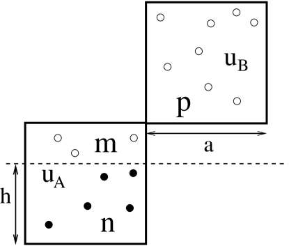
Figure 3: A double cell consisting of two subcells for collision along the upward diagonal direction $\mbox{\boldmath$\sigma$}_{3}$ as defined in fig. 1. $u_{A}$ is the component of the mean velocity projected on $\mbox{\boldmath$\sigma$}_{3}$ of the $n+m=N_{A}$ particles in the left subcell. The projected mean velocity of the $p=N_{B}$ particles in the upper right subcell is given by $u_{B}$. A line divides the lower cell at height $h$, $0\leq h\leq a$.

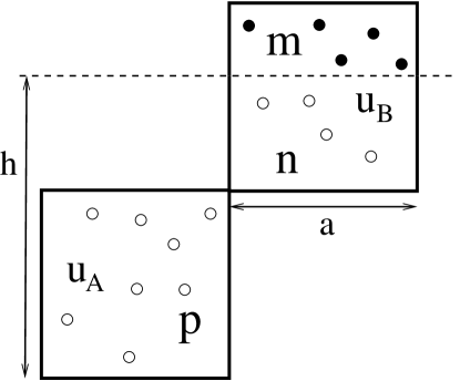
Figure 4: A double cell consisting of two subcells for collision along the upward diagonal direction $\mbox{\boldmath$\sigma$}_{3}$ as defined in fig. 1. $u_{A}$ is the component of the mean velocity projected on $\mbox{\boldmath$\sigma$}_{3}$ of the $p=N_{A}$ particles in the lower left subcell. The projected mean velocity of the $n+m=N_{B}$ particles in the upper right subcell is given by $u_{B}$. A line divides the upper cell at height $h$, $a\leq h\leq 2a$.

Both diagonal collisions along $\mbox{\boldmath$\sigma$}_{3}$ and $\mbox{\boldmath$\sigma$}_{4}$ in fig. 1 will also transfer x-momentum over a horizonal diagonal line. Only the contribution from the upward diagonal, $\mbox{\boldmath$\sigma$}_{3}$, will be discussed here, since the contribution from the down-wards diagonal gives the same result for symmetry reasons. It is neccessary to distinguish between the two cases depicted in figs. 3 and 4: where (A) the dividing line goes through the lower cell and, (B) where the line goes through the upper cell. Only both contributions together will give the correct result with the same structure than eq. (80).

First, case A is considered. The change of x-momentum of the particles described by full circles in fig. 3 is given as

$$\langle{\Delta}p_{x}\rangle_{nmp}^{A}=\left\langle\left\langle p_{A}\,\sum_{j=1}^{n}\Delta v_{i,x}\right\rangle_{V}\right\rangle_{Y}$$ (81)

where the upper index, $A$, denotes upward diagonal collisions for situation A. The average over the particle height $\langle...\rangle_{Y}$ and the velocity distribution $\langle...\rangle_{V}$ differs from the previous definition eqs. (65,66)

$$\langle...\rangle_{V} = \int_{-\infty}^{\infty}\,...f_{N,x}f_{N,y}\,dv_{i,x}^{n+m+p}\,dv_{i,y}^{n+m+p}$$ (82)

$$\langle...\rangle_{Y} = {1\over h^{n}}\int_{0}^{h}\,dy_{i}^{n}{1\over(a-h)^{m}}\int_{h}^{a}\,dy_{i}^{m}{1\over a^{p}}\int_{a}^{2a}\,...\,dy_{i}^{p}$$ (83)

the velocity average now involves the $y$-component of the particle velocities as well.

The acceptance probability $p_{A}$ is again given by eq. (12) and proportional to $\theta(\Delta u)$ which however has now a different form,

$$\Delta u=u_{A}-u_{B}={1\over N_{A}}\sum_{i=1}^{n+m}{v_{i,x}+v_{i,y}\over\sqrt{2}}-{1\over N_{B}}\sum_{i=n+m+1}^{n+m+p}{v_{i,x}+v_{i,y}\over\sqrt{2}}\,.$$ (84)

The particle number in the bottom left cell is $N_{A}=n+m$, and $N_{B}=p$, is the particle number in the top right cell. Using the exponential representation (20,21) for the $\theta$-function, and the upward collision rule (2) to redefine $\Delta v_{i,x}=u_{x}+u_{y}-v_{i,x}-v_{i,y}$, one finds

$$\langle{\Delta}p_{x}\rangle_{nmpq}^{A}=AN_{A}N_{B}$$

$$\times\left\langle\left\langle\int_{0}^{\infty}dc\int_{-\infty}^{\infty}{dk\over 2\pi}{\rm e}^{ik(\Delta u-c)}\Delta u\,\sum_{j=1}^{n+p}(u_{x}+u_{y}-v_{j,x}-v_{j,y})\right\rangle_{V}\right\rangle_{Y}$$ (85)

This expression is evaluated using similar substitutions and approximations than for horizontal collisions. After performing all averages one obtains the momentum transfer for fixed particle numbers $N_{A}$, $N_{B}$ (in linear order in the shear rate $\dot{\gamma}$):

$$\langle\langle{\Delta}p_{x}\rangle\rangle_{N_{A},N_{B}}^{A}={A\dot{\gamma}a\over 12}\sqrt{k_{B}T\over 2\pi\gamma}\,\left[(N_{A}-1)\left(1-{N_{B}\over N_{A}}\right)+14N_{A}N_{B}\right]$$ (86)

A similar calculation for case B where the dividing line cuts the top right cell, see fig. 4, results in

$$\langle\langle{\Delta}p_{x}\rangle\rangle_{N_{A},N_{B}}^{B}={A\dot{\gamma}a\over 12}\sqrt{k_{B}T\over 2\pi\gamma}\,\left[(N_{B}-1)\left(1-{N_{A}\over N_{B}}\right)+14N_{A}N_{B}\right]$$ (87)

By averaging both results, one finds the momentum transfer for the upward (U) diagonal collision for $N_{A}\geq 1$ and $N_{B}\geq 1$:

$$\langle\langle{\Delta}p_{x}\rangle\rangle_{N_{A},N_{B}}^{U} = {1\over 2}\left(\langle\langle{\Delta}p_{x}\rangle\rangle_{N_{A},N_{B}}^{A}+\langle\langle{\Delta}p_{x}\rangle\rangle_{N_{A},N_{B}}^{B}\right)$$ (88)

$$= {A\dot{\gamma}a\over 6}\sqrt{k_{B}T\over 2\pi\gamma}\,\left[7N_{A}N_{B}+{(N_{A}-N_{B})^{2}\over 4N_{A}N_{B}}\right]$$

This expression is symmetric in $N_{A}$ and $N_{B}$, as it should be, and has the same general structure than eq. (80). Finally, this result is multiplied by two to account for the contribution from the downward diagonal and added together with the result for horizontal collisions using the weight factors $w$ and $w_{d}$ for horizontal and diagonal collisions, respectively. The total average momentum transfer is:

$$\langle\langle{\Delta}p_{x}\rangle\rangle_{N_{A},N_{B}}=$$

$${A\dot{\gamma}a\over 12}\sqrt{k_{B}T\over 2\pi\gamma}\,\left[(28w_{d}+8w)N_{A}N_{B}+(w_{d}+2w){(N_{A}-N_{B})^{2}\over N_{A}N_{B}}\right]$$ (89)

Now, one can derive the collisional part to the kinematic viscosity, $\nu_{coll}$, which is proportional to the momentum transfered per time and length

$${\langle\Delta p_{x}\rangle\over 2a\,\tau}=\dot{\gamma}\,\nu_{coll}\,\rho$$ (90)

$\rho=M/a^{2}$ is the density of our two-dimensional fluid. Replacing the particle numbers $N_{A}$ and $N_{B}$ by the average particle number per cell, $M$ and setting $w=1/4$ and $w_{d}=1/2$, one gets

$$\nu_{coll}={a^{2}\over 3\tau}A\sqrt{k_{B}T\over\pi}\,M^{3/2}$$ (91)

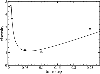
Figure 5: Total viscosity $\nu$ as a function of time step $\tau$ for small collision rate. The symbols are numerical results obtained by evaluating Green-Kubo relations for $M=3$. The solid line is the theoretical result, $\nu=\nu_{coll}+\nu_{kin}$ from eqs. (61,91). Parameters: $L=64a$, $M=5$, $k_{B}T=1$, and $A=1/60$.

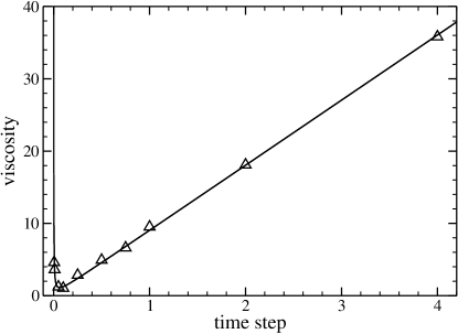
Figure 6: Same as fig. 5: total viscosity $\nu=\nu_{coll}+\nu_{kin}$ as a function of time step $\tau$, but for larger $\tau$, and compared to the theoretical result.

for not too small mean particle number per cell, $M\geq 2$. Figs. 5 and 6 compare the theoretical result for the total viscosity, $\nu=\nu_{coll}+\nu_{kin}$ from eqs. (61,91) with numerical results obtained by evaluating Green-Kubo relations for stress autocorrelation functions (for numerical details see refs. [17, 20]). One sees that the agreement at small and large mean free paths is very good. The small deviations at intermediate mean free path are within the error bars of the data. However, there is another possibility; in regular SRD it was found, [24], that at $\lambda\ll a$ corrections due to the violation of molecular chaos become relevant in $\nu_{kin}$, but not in $\nu_{coll}$. These effects are large for very small $\lambda$, but in this limit they are irelevant for the total viscosity because it is dominated by $\nu_{coll}$. Hence, if at all, one would see these deviations only at intermediate mean free paths. It is possible that there are similar deviations for the current model which could show at intermediate $\lambda$.

There is a simple argument for the structure of expression (91): Collisions “smear out” momentum over a distance of order cell size $a$ in one time step $\tau$. The kinematic viscosity is the coefficient of momentum diffusion which in analogy to a random walk is defined by the “hopping ” distance $a$ per time step as $D\sim a^{2}/\tau$. However, the collisions occur with some collision rate which is proportional to the thermal average of the acceptance probability given by

$$\langle p_{A}\rangle=A\,\langle\theta(\Delta u)\,\Delta uN_{A}N_{B}\rangle\sim A\,\sqrt{k_{B}T}\,M^{3/2}$$ (92)

Therefore, one would expect

$$\nu_{coll}\sim{a^{2}\over\tau}\langle p_{A}\rangle\sim{a^{2}\over\tau}\,A\,\sqrt{k_{B}T}\,M^{3/2}$$ (93)

which is exactly what was found. A similar argument can be made for the kinetic part of the viscosity. The analogy to a random walk predicts $\nu_{kin}\sim\lambda^{2}/\tau$ since momentum is now only “hopping” a distance of order mean free path $\lambda=\tau\sqrt{k_{B}T}$. In addition, it is clear that at $p_{A}\rightarrow 0$ there is almost no collisions, the momentum is travelling huge distances and the kinetic viscosity becomes very large. This can be described by an additional factor $1/\langle p_{A}\rangle$ and one obtains,

$$\nu_{kin}\sim{1\over\langle p_{A}\rangle}{\lambda^{2}\over\tau}\sim{k_{B}T\tau\over\langle p_{A}\rangle}\sim{\tau\over A}\sqrt{k_{B}T}\,M^{-3/2}$$ (94)

which, apart from a small correction term, agrees with what was derived rigorously, eq. (61). Using this conceptual insight, one can easily predict the general form of these expressions for arbitrary acceptance probabilities without actually going through tedious derivations.

6 Results for other models

6.1 Large collision rate, $A\rightarrow\infty$

The calculation of the previous sections are easily modified to treat the limit of large collision parameter $A\rightarrow\infty$, where the acceptance probability is simply $p_{A}=\theta(\Delta u)$. One finds,

$$\nu_{kin}^{\infty}={k_{B}T\,\tau\over 2}\,\left({6M+1-{\rm e}^{-2M}\over 2M-1+{\rm e}^{-2M}}\right)$$ (95)

for the kinetic viscosity if ideal gas-like fluctuations are assumed. The exponential terms come from averaging over the particle number fluctuations assuming a Poisson-distribution. This assumption is correct for an ideal gas, but not for the current model with a non-ideal equation of state, which has smaller fluctuations. Furthermore, it was shown that the density fluctuations in the limit of large $A$ are even smaller than predicted by the equation of state [19]. Given the small size of the exponential terms $\sim{\rm e}^{-2M}$ for typical particle numbers $M$ between three and twenty, the fluctuation corrections, i.e. the exponential terms, can be safely neglected.

By modifying the non-equilibrium calculation scheme of section 5, one obtains the average momenum transfer in shear flow for $N_{A}\geq 1$, $N_{B}\geq 1$ as

$$\langle\langle{\Delta}p_{x}\rangle\rangle_{N_{A},N_{B}}=$$

$${a\dot{\gamma}\over 24(N_{A}+N_{B})}\,\left[(14w_{d}+4w)N_{A}N_{B}+(w_{d}+2w)(N_{A}+N_{B}-2)\right]$$ (96)

Ignoring particle number fluctuations by setting $N_{A}=N_{B}=M$, substituting $w=1/4$, $w_{d}=1/2$, the collisional viscosity follows from eq. (90),

$$\nu_{coll}^{\infty}={a^{2}\over 12\tau}\left[1+{1\over 4M}\left(1-{1\over M}\right)\right]$$ (97)

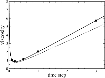
Figure 7: Total viscosity $\nu=\nu_{coll}+\nu_{kin}$ as a function of time step $\tau$ for large collision rate, $A\rightarrow\infty$. The symbols are numerical results obtained by evaluating Green-Kubo relations for $M=3$. The solid line is the theoretical result from eqs. (95,97), for $M=3$. The dashed line is the theoretical result for $M=10$. Parameters: $L=64a$, $k_{B}T=1$, and $A\rightarrow\infty$.

Fig. 7 shows excellent agreement of simulation data for $M=3$ from ref. [19] with the theoretical results for the total viscosity $\nu=\nu_{kin}+\nu_{coll}$ from eqs. (95, 97). One sees that the viscosity is basically independent of the particle number $M$ at small mean free path.

6.2 Transport coefficients for a binary mixture

In [18] a multi-component version of the current collision model was introduced. Consider a binary system with two types of particles, A and B. In order to obtain phase separation, a repulsion between different kind of the particles was implemented; but there is no repulsion among particles of the same kind. This is done in the following way: Suppose a double cell is selected for a possible collision. A-particles in cell 1 can undergo collisions with B-particles from cell 2. For symmetry reasons, B-particles from cell 1 are also checked for possible collision with A-particles in cell 2. The rules and probabilities for these collisions are exactly the same as in the one-component situation. This means, most of the results derived above can be used with only minor modifications.

$M_{A}=\langle N_{A}\rangle$ is the average number of A-particles in a cell of size $a$, $M_{B}=\langle N_{B}\rangle$ is the average of B-particles in such a cell. The total particle density in a cell is now given by $\rho=(M_{A}+M_{B})/a^{2}$. While using eqs. (16) to (3.1) for diffusion calculations one has to distinguish whether the tagged particle is of the A or B type. For the self-diffusion of A-particles one has to set $n=N_{A}$ and $m=N_{B}$ in eq. (18) for $K^{l}_{nm}$, but $n=N_{B}$ and $m=N_{A}$ in $K^{r}_{nm}$ which, because of the symmetry $K^{r}_{nm}=K^{l}_{mn}$, leads to $K_{nm}=K^{l}_{N_{A}N_{B}}$. The corresponding results for the auxiliary variables $g_{H}$, $g_{U}$ and $g$ are not symmetric with respect to the particle numbers $N_{A}$ and $N_{B}$, and a short calculation gives $g_{H}^{A}=1-2\phi^{A}$, $g_{U}^{A}=1-\phi^{A}$, and $g^{A}=1-\phi^{A}$ with

$$\phi^{A}=A\sqrt{k_{B}T\over 2\pi\gamma}\left(M_{A}+M_{B}-1+{M_{B}\over M_{A}}\right)$$ (98)

and $\gamma=1/M_{A}+1/M_{B}$ where the actual numbers $N_{A}$, $N_{B}$ were already replaced by their average values, $M_{A}$ and $M_{B}$, respectively. Similar considerations hold for the diffusion of B particles and one obtains the diffusion coefficient for A and B particles, respectively,

$$D_{A} = k_{B}T\tau\left({1\over\phi_{A}}-{1\over 2}\right)$$

$$D_{B} = k_{B}T\tau\left({1\over\phi_{B}}-{1\over 2}\right)\;\;{\rm with}$$

$$\phi^{B} = A\sqrt{k_{B}T\over 2\pi\gamma}\left(M_{A}+M_{B}-1+{M_{A}\over M_{B}}\right)$$ (99)

Both particles diffuse the same way only if $M_{A}=M_{B}$. In this case the diffusion coefficient $D=D_{A}=D_{B}$ agrees with the one for the single-component model, eq. (38). If there is less A than B particles, the diffusion of A particles is slower even if the masses of both particles are the same as assumed here. This is physically plausible, since a single A-particle in a sea of B particles will be backscattered very often whereas the many B-particles keep going and are less affected by the collisions. Fig. 8 plots the ratio of the two diffusion coefficients $D_{A}/D_{B}$ as a function of the averaged relative particle number difference, $\Delta\rho=(M_{A}-M_{B})/(M_{A}+M_{B})$ for fixed total number $M=M_{A}+M_{B}$. $\Delta\rho$ was only varied in a range were both particle numbers $M_{A}$ and $M_{B}$ are always larger or equal to one because density fluctuations become significant at smaller particle numbers but are neglected in the theory. For a total number of $M=5$ and $M_{A}=1$, $M_{B}=4$ one sees that B-particles diffuse about twice as fast than A-particles.

Finally, the kinetic and collisional viscosities are determined by applying concepts from the previous sections, and one finds

$$\nu_{kin}^{bin} = k_{B}T\,\tau\left\{{1\over A}\sqrt{\pi\over 2k_{B}T}[M_{A}M_{B}(M_{A}+M_{B})]^{-1/2}-{1\over 2}\right\}$$

$$\nu_{coll}^{bin} = {Aa^{2}\over 3\tau}\sqrt{k_{B}TM_{A}M_{B}\over 2\pi(M_{A}+M_{B})^{3}}\left[4M_{A}M_{B}+{(M_{A}-M_{B})^{2}\over 4M_{A}M_{B}}\right]$$ (100)

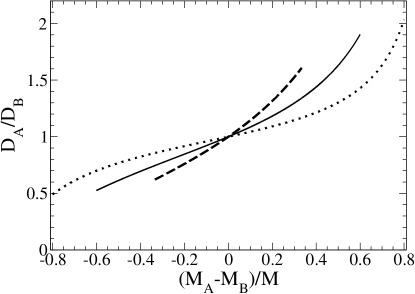
Figure 8: Ratio of the diffusion coefficient for A and B particles, $D_{A}/D_{B}$, as a function of averaged relative particle number $\Delta\rho=(M_{A}-M_{B})/M$ for fixed total number $M=M_{A}+M_{B}$. The dashed line is the theoretical result from eqs. (99), for $M=3$. The solid line is for $M=5$, and the dotted one is for $M=10$. Parameters: $k_{B}T=1$, $A=1/60$, $\tau=1$, $M_{A}\geq 1$, $M_{B}\geq 1$.

7 Conclusion

In this paper, I have presented a detailed, systematic derivation of the transport coefficients of a multi-particle collision model for fluid flow with a non-ideal equation of state. Similar calculations have been published before, but to my knowledge, this is the first derivation which accounts for velocity-biased collision rules in MPC. Analytic expressions for the self-diffusion coefficient, and the shear viscosity are obtained, and very good agreement is found with numerical results at small and large mean free paths. For the analysis of the collisional contribution to the viscosity, an earlier scheme was improved which can now be used to derive possible shear thinning or thickening. The general formalism was also applied to a binary collision model with a miscibility gap. General arguments for the scaling of the transport coefficients with temperature and particle number as a function of the collision rule are given. This allows one to predict without tedious derivations how the transport coefficients change if the collision rule is modified.

For the current collision rule, the viscosity turns out to be proportional to the square root of temperature as in a real gas. It is shown that at large mean free path, the viscosity and the diffusion coefficient are exactly equal, resulting in a Schmidt number of one in this limit.

8 Acknowledgement

Acknowledgement is made to the Donors of the American Chemical Society Petroleum Research Fund for partial support of this research. I thank F. Jülicher for his hospitality at the MPI-PKS. I would like to thank E. Tüzel for discussions and help in the initial stage of this work, and D. Kroll and T. Pilling for many discussions and proof-reading of the manuscript. I also thank J. Yeomans for providing unpublished results about shear-thinning.

References

• [1] P.J. Hoogerbrugge and J.M.V.A. Koelman, Europhys. Lett. 19, 155 (1992).
• [2] P. Espanol, Phys. Rev. E 57, 2930 (1998).
• [3] J.J. Monaghan, Rep. Prog. Phys. 68, 1703 (2005).
• [4] G.A. Bird, Molecular Gas Dynamics, Clarendon Press, Oxford, 1976.
• [5] F.J. Alexander and A.L. Garcia, Computers in Fluids 11, 588 (1997).
• [6] A. Malevanets and R. Kapral, J. Chem. Phys. 110, 8605 (1999).
• [7] A. Malevanets and R. Kapral, J. Chem. Phys. 112, 7260 (2000).
• [8] T. Ihle and D.M. Kroll, Phys. Rev. E 63, 020201(R) (2001).
• [9] T. Ihle and D.M. Kroll, Phys. Rev. E 67, 066705 (2003); Phys. Rev. E 67, 066706 (2003).
• [10] E. Tรผzel, M. Strauss, T. Ihle and D.M. Kroll, Phys. Rev. E 68, 036701 (2003).
• [11] C.M. Pooley and J.M. Yeomans, J. Phys. Chem. B 109, 6505 (2005).
• [12] J.T. Padding, A. Wysocki, H. Lรถwen, and A.A. Louis, J. Phys.: Conds. Matter 17, S3393 (2005).
• [13] A. Lamura and G. Gompper, European Phys. J. E 9, 477 (2002).
• [14] E. Allahyarov and G. Gompper, Phys. Rev. E 66, 041805 (2002)
• [15] M. Ripoll, K. Mussawisade, R.G. Winkler, and G. Gompper, Europhys. Lett. 68, 106 (2004).
• [16] R.G. Winkler, K. Mussawisade, M. Ripoll, and G. Gompper, J. Phys.: Condens. Matter 16, S3941 (2004).
• [17] T. Ihle, E. Tรผzel, and D.M. Kroll, Europhys. Lett. 73, 664 (2006)
• [18] E. Tรผzel, G. Pan, T. Ihle and D.M. Kroll, Europhys. Lett. 80 40010 (2007).
• [19] E. Tรผzel, T. Ihle, and D.M. Kroll, Mathematics and Computers in Simulation 72, 232 (2006)
• [20] T. Ihle and E. Tรผzel, cond-mat/0610350, Prog. Comp. Fluid Dyn. 2008, in press.
• [21] T. Ihle, E. Tรผzel, and D.M. Kroll, Phys. Rev. E 72, 046707 (2005)
• [22] J.F. Ryder and J.M. Yeomans, J. Chem. Phys. 125, 194906 (2006).
• [23] J.F. Ryder, Ph.D. Thesis, University of Oxford (2005).
• [24] E. Tรผzel, T. Ihle, and D.M. Kroll, Phys. Rev. E 74 056702 (2006).