Three-body structure of low-lying ¹²Be states

Abstract

We investigate to what extent a description of ¹²Be as a three-body system made of an inert ¹⁰Be-core and two neutrons is able to reproduce the experimental ¹²Be data. Three-body wave functions are obtained with the hyperspherical adiabatic expansion method. We study the discrete spectrum of ¹²Be, the structure of the different states, the predominant transition strengths, and the continuum energy spectrum after high energy fragmentation on a light target. Two $0^{+}$, one $2^{+}$, one $1^{-}$ and one $0^{-}$ bound states are found where the first four are known experimentally whereas the $0^{-}$ is predicted as an isomeric state. An effective neutron charge, reproducing the measured $B(E1)$ transition and the charge rms radius in ¹¹Be, leads to a computed $B(E1)$ transition strength for ¹²Be in agreement with the experimental value. For the $E0$ and $E2$ transitions the contributions from core excitations could be more significant. The experimental ¹⁰Be-neutron continuum energy spectrum is also well reproduced except in the energy region corresponding to the $3/2^{-}$ resonance in ¹¹Be where core excitations contribute.

I Introduction

The second lightest bound nucleus in the $N=8$ isotonic chain is ¹²Be, placed in the nuclear chart just above the widely investigated borromean ¹¹Li nucleus. These two nuclei are essential to understand the breakdown of the $N=8$ shell closure when the dripline is approached. The parity inversion in ¹¹Be, already known in the early 70’s ajz75 , is a clear indication of this fact. The particle unstable nucleus ¹⁰Li should in principle have the same neutron configuration as ¹¹Be. Several theoretical works also predicted the existence of an intruder low-lying $s$-wave state bar77 ; joh90 ; tho94 . The available experimental data concerning the ground state properties of ¹⁰Li are however controversial, although most of them point towards the existence of such low-lying virtual $s$-state kry93 ; you94 ; abr95 ; zin95 . This result has been confirmed in the recent work jep06 .

These properties of ¹¹Be and ¹⁰Li clearly suggest that the $p-sd$ shell gap is reduced when approaching the neutron dripline, leading to a structure of ¹²Be and ¹¹Li with a large contribution from $sd$ configurations. This has been confirmed theoretically and experimentally for both ¹²Be bar76 ; for94 ; nav00 ; pai06 and ¹¹Li tho94 ; gar02 ; zin97 .

The ¹¹Li properties have been successfully described by use of three-body models that freeze the degrees of freedom of the ⁹Li core zhu93 ; gar01 . It is then tempting to follow a similar procedure to investigate ¹²Be. In fact, although ¹²Be is not borromean, ¹¹Be is considered to be the prototype of one-neutron halo nuclei fuk91 ; ann93 ; kel95 , and therefore a description of ¹²Be as a ¹⁰Be core surrounded by two neutrons appears as a good first approach.

An important advantage of ¹²Be compared to ¹¹Li is that the properties of ¹¹Be are are much better known than the ones of ¹⁰Li, and therefore the uncertainties arising from the core-neutron interaction should in principle be smaller. However, while in ¹¹Li the ⁹Li core is spherical, the ¹⁰Be core in ¹²Be is deformed, and as such one of the essential reasons for the shell closure breaking in ¹²Be. The ground state in ¹¹Be contains an important contribution from core excited configurations tee77 . Different theoretical calculations have estimated this contribution, and the results range from 40% in ots93 to 10% in esb95 ; des97 , passing through 20% in vin95 ; nun96 . Recent experimental data for99 ; win01 are consistent with a 16% admixture of core excitation in the ¹¹Be ground state wave function.

As a consequence of this, a description of ¹²Be as an inert core surrounded by two neutrons is quite questionable, and the role played by the core excitations is an important issue to be clarified. In nun96b a hyperspherical expansion of the three-body wave function was used to obtain the ground state of ¹²Be including core excitations. It was found that simultaneous fitting of the experimental ground state energy and the experimental longitudinal momentum distribution of ¹⁰Be after high energy fragmentation of ¹²Be, required a strong core excited component in the wave function ($\approx 42$%).

However, after publication of this work additional experimental information about the spectrum of ¹²Be became available. A bound $2^{+}$ state and a bound $1^{-}$ state were found with excitation energies of 2.10 MeV alb78 ; iwa00 and 2.68 MeV iwa00b , respectively. Also the existence of a second $0^{+}$ bound state with excitation energy of 2.24 MeV was already envisaged shi01 (later on confirmed shi03 ). Also, the (¹²Be,¹¹Be$\gamma$) one neutron removal measurements at the NSCL nav00 allowed a direct estimate of the $\langle^{11}$Be$(j^{\pi})|^{12}$Be(gs)$\rangle$ spectroscopic factors. All this new data lead the authors of nun96b to review their calculations nun02 . They found that a reasonable simultaneous matching of the data required a significant reduction of the core deformation, and hence a smaller contribution from core excitation ($\approx 20$%).

Very recently new experimental data on ¹²Be have been provided pai06 . Specially interesting is the continuum relative energy spectrum for ¹⁰Be+$n$ after high energy breakup of ¹²Be on a carbon target. This invariant mass spectrum is known to be very sensitive to the final state interaction gar97 ; gar99 , and therefore, in our case, to the properties of the unbound ¹¹Be states. A reliable calculation of the spectrum requires inclusion of the ¹⁰Be-neutron continuum states together with core-neutron resonances. This energy spectrum is then a very useful observable to investigate the role played by the ¹⁰Be-neutron interaction, and to constrain the remaining uncertainties in the structure of ¹²Be.

In previous ¹²Be three-body calculations (¹⁰Be+$n$+$n$) tho94 ; nun96b ; nun02 the wave functions were obtained using the hyperharmonic expansion. The employed neutron-core potentials were chosen to reproduce the bound ¹¹Be states and perhaps the first resonance at 1.78 MeV (excitation energy) but higher unbound states were ignored. This method is not the most efficient for a non-borromean system like ¹²Be, where two of the two-body subsystems have bound states. This is because an infinite hyperharmonic basis is in principle needed to reproduce the correct two-body asymptotics dan98 . The convergence of the hyperharmonic expansion is slow, and in practice the energies and rms radii are obtained after extrapolation of the numerical results tho94 ; nun96b ; nun02 where the basis is progressively increased up to a maximum value of the hypermomentum $K_{max}=20$ for the ground state, and $K_{max}=12$ for the excited states.

In the present context the hyperspheric adiabatic expansion method nie01 is more appropriate. This method solves the Faddeev equations in coordinate space, treating symmetrically the three two-body interactions such that each of them only appears in its natural coordinates. This makes the method specially suitable for non-borromean systems like ¹²Be, where more than one two-body subsystem has bound states. Also the method permits the use of much larger values of the hypermomentum quantum number which guaranties convergence of the results.

The main goal of the present work is to assess to what extent a three-body model with an inert ¹⁰Be-core is able to reproduce the existing rather large amount of both old and new experimental data concerning ¹²Be, i.e. the ¹²Be spectrum, the $E1$ and $E2$ transition strengths iwa00 ; iwa00b ; shi07 , the ${\cal M}$(E0) shi07 and the measured invariant mass spectrum pai06 . The two-body potentials to be used in the calculations are fitted to reproduce the available two-body experimental data, in particular, the ¹¹Be data. In this sense, although the ¹⁰Be core is considered an inert particle with spin and parity 0⁺, the employed two-body interactions phenomenologically account for all effects of core excitation appearing in the corresponding channel. In particular it is interesting to know if the weakly bound excited states can be understood as halo states and perhaps can be better described in a three-body model than the relatively well bound ground state. Relations between various quantities can be tested and new properties predicted. For this the hyperspheric adiabatic expansion method is well suited. By comparing computed results and available data we can establish how large the contributions must be from inclusion of core excitations.

The paper is organized as follows. In section II we very briefly describe the basis of the three-body method. The different two-body interactions used in the calculations are detailed in section III. The results are shown in sections IV, V, and VI, where we discuss the spectrum and structure of ¹²Be, the electromagnetic transition strengths, and the invariant mass spectrum after high-energy breakup, respectively. We finish in section VII with a summary and the conclusions. In the appendix some remarks about the $E1$ and $E2$ operators are given.

II Theoretical formulation

We assume ¹²Be can be described as a three-body system made by a ¹⁰Be core and two neutrons. The wave functions for the different bound states are obtained with the hyperspherical adiabatic expansion method. A detailed description of the method can be found in nie01 .

This method solves the Faddeev equations in coordinate space. The wave functions are computed as a sum of three Faddeev components $\psi^{(i)}(\bm{x}_{i},\bm{y}_{i})$ ($i$=1,2,3), each of them expressed in one of the three possible sets of Jacobi coordinates $\{\bm{x}_{i},\bm{y}_{i}\}$. Each component is then expanded in terms of a complete set of angular functions $\{\phi_{n}^{(i)}\}$

$$\psi^{(i)}={1\over\rho^{5/2}}\sum_{n}f_{n}(\rho)\phi_{n}^{(i)}(\rho,\Omega_{i});(\Omega_{i}\equiv\{\alpha_{i},\Omega_{x_{i}},\Omega_{y_{i}}\}),$$ (1)

where $\rho=\sqrt{x^{2}+y^{2}}$, $\alpha_{i}=\arctan({x_{i}/y_{i}})$, $\Omega_{x_{i}}$, and $\Omega_{y_{i}}$ are the angles defining the directions of $\{\bm{x}_{i}$ and $\bm{y}_{i}\}$. Writing the Faddeev equations in terms of these coordinates, they can be separated into angular and radial parts:

$$\hat{\Lambda}^{2}\phi_{n}^{(i)}+\frac{2m\rho^{2}}{\hbar^{2}}V_{jk}(x_{i})\left(\phi_{n}^{(i)}+\phi_{n}^{(j)}+\phi_{n}^{(k)}\right)=\lambda_{n}(\rho)\phi_{n}^{(i)}$$ (2)

$$\left[-\frac{d^{2}}{d\rho^{2}}+\frac{2m}{\hbar^{2}}(V_{3b}(\rho)-E)+\frac{1}{\rho^{2}}\left(\lambda_{n}(\rho)+\frac{15}{4}\right)\right]f_{n}(\rho)$$ (3)

$$+\sum_{n^{\prime}}\left(-2P_{nn^{\prime}}\frac{d}{d\rho}-Q_{nn^{\prime}}\right)f_{n^{\prime}}(\rho)=0$$

where $V_{jk}$ is the two-body interaction between particles $j$ and $k$, $\hat{\Lambda}^{2}$ is the hyperangular operator nie01 and $m$ is the normalization mass. In Eq.(3) $E$ is the three-body energy, and the coupling functions $P_{nn^{\prime}}$ and $Q_{nn^{\prime}}$ are given for instance in nie01 . The potential $V_{3b}(\rho)$ is used for fine tuning to take into account all those effects that go beyond the two-body interactions. In the present cases it is rather small and unless the opposite is explicitly said, this three-body potential is taken equal to zero.

It is important to note that the angular functions used in the expansion (1) are precisely the eigenfunctions of the angular part of the Faddeev equations. Each of them is in practice obtained by expansion in terms of the hyperspherical harmonics. Obviously this infinite expansion has to be cut off at some point, maintaining only the contributing components.

The eigenvalues $\lambda_{n}(\rho)$ in Eq.(2) enter in the radial equations (3) as a basic ingredient in the effective radial potentials. Accurate calculation of the $\lambda$-eigenvalues requires, for each particular component, a sufficiently large number of hyperspherical harmonics. In other words, the maximum value of the hypermomentum ($K_{max}$) for each component must be large enough to assure convergence of the $\lambda$-functions in the region of $\rho$-values where the $f_{n}(\rho)$ wave functions are not negligible.

Finally, the last convergence to take into account is the one corresponding to the expansion in Eq.(1). Typically, for bound states, this expansion converges rather fast, and usually three or four adiabatic terms are already sufficient.

III Two-body interactions

It is known that for weakly bound systems, like for instance ⁶He or ¹¹Li, the short distance behaviour of the two-body potentials is relatively unimportant as long as they reproduce the low-energy scattering data. Then the essential three-body properties can be described zhu93 .

III.1 Neutron-neutron potential

For the neutron-neutron interaction we use a simple potential reproducing the experimental $s$- and $p$-wave nucleon-nucleon scattering lengths and effective ranges. It contains central, spin-orbit ($\bm{\ell}\cdot\bm{s}$), tensor ($S_{12}$) and spin-spin ($\bm{s}_{1}\cdot\bm{s}_{2}$) interactions, and is explicitly given as gar04

$$V_{nn}(r)=37.05e^{(-(r/1.31)^{2})}$$ (4)

$$-7.38e^{(-(r/1.84)^{2})}-23.77e^{(-(r/1.45)^{2})}\bm{\ell}\cdot\bm{s}$$

$$+\left(49.40e^{(-(r/1.31)^{2})}+29.53e^{(-(r/1.84)^{2})}\right)\bm{s}_{1}\cdot\bm{s}_{2}$$

$$+7.16e^{(-(r/2.43)^{2})}S_{12},$$

where $\bm{\ell}$ is the relative orbital angular momentum between the two neutrons, and $\bm{s}=\bm{s}_{1}+\bm{s}_{2}$ is the total spin. The strengths are in MeV and the ranges in fm. We will refer to this potential as gaussian neutron-neutron potential.

To test the role played by the short-distance properties of the neutron-neutron interaction, for some specific cases, we are also using the more sophisticated $v_{8}$ version of the nucleon-nucleon Argonne potential wir95 . This is a non-relativistic potential reproducing proton-proton and neutron-proton scattering data for energies from 0 to 350 MeV, neutron-neutron low-energy scattering data, as well as the deuteron properties.

III.2 Neutron-¹⁰Be potential

For the neutron-core interaction we have constructed an $\ell$-dependent potential of the form:

$$V^{(\ell)}(r)=V^{(\ell)}_{c}(r)+V^{(\ell)}_{so}(r)\bm{\ell}\cdot\bm{s}_{n},$$ (5)

where $\bm{\ell}$ is the neutron-core relative orbital angular momentum and $\bm{s}_{n}$ is the spin of the neutron.

Table 1: Strengths (in MeV) and ranges (in fm) of the central and spin-orbit gaussian potentials ($V_{c}^{(\ell)}(r)=S_{c}^{(\ell)}e^{-(r/b_{c}^{(\ell)})^{2}}$, $V_{so}^{(\ell)}(r)=S_{so}^{(\ell)}e^{-(r/b_{so}^{(\ell)})^{2}}$ ) entering in Eq.(5) for the four interactions used in the calculations. For $d$-waves the radial potentials are made as the sum of two gaussians, whose strengths and ranges are given by the corresponding two rows in the table. In Potential $IV$ the acronym “P.E.P”. refers to the Phase Equivalent Potential used in this case for $s$ and $p$ waves (see text).

		$W_{I}$	$W_{II}$	$W_{III}$	$W_{IV}$
$s$-waves	$S_{c}^{(\ell=0)}$	$-8.40$	$-5.78$	$-8.40$	P.E.P.
	$b_{c}^{(\ell=0)}$	3.5	4.5	3.5	P.E.P.
$p$-waves	$S_{c}^{(\ell=1)}$	40.0	40.0	40.0	P.E.P.
	$b_{c}^{(\ell=1)}$	3.5	3.5	3.5	P.E.P.
	$S_{so}^{(\ell=1)}$	63.52	63.52	63.52	P.E.P.
	$b_{so}^{(\ell=1)}$	3.5	3.5	3.5	P.E.P.
$d$-waves	$S_{c}^{(\ell=2)}$	$-26.28$	$-26.28$	$-26.28$	$-26.28$
		$-79.6$	$-79.6$	$-33.39$	$-79.6$
	$b_{c}^{(\ell=2)}$	3.5	3.5	3.5	3.5
		1.7	1.7	2.5	1.7
	$S_{so}^{(\ell=2)}$	$-17.52$	$-17.52$	$-17.52$	$-17.52$
		79.6	79.6	33.39	79.6
	$b_{so}^{(\ell=2)}$	3.5	3.5	3.5	3.5
		1.7	1.7	2.5	1.7

The central $(V^{(\ell)}_{c}(r))$ and spin-orbit $(V^{(\ell)}_{so}(r))$ radial potentials are assumed to have a gaussian shape. In this work four different ¹⁰Be-neutron potentials (labeled as $I$, $II$, $III$, and $IV$) will be used. Their parameters for $\ell$=0, 1, and 2 are given in table 1, and they are adjusted to reproduce the spectrum of ¹¹Be. Contributions from partial waves with $\ell>2$ are negligibly small and not included.

Potential I is built as follows: the range of the interactions is taken equal to 3.5 fm, that is the sum of the rms radius of the core and the radius of the neutron. For $s$-waves the strength is fixed to fit the experimental neutron separation energy of the $1/2^{+}$-state in ¹¹Be ($-0.504$ MeV ajz90 ). For $p$-waves the two free parameters (central and spin-orbit strengths) are adjusted to reproduce the experimental neutron separation energy of the $1/2^{-}$-state in ¹¹Be ($-0.184$ MeV ajz90 ), and simultaneously push up the $3/2^{-}$ state, which is forbidden by the Pauli principle, since it is occupied by the four neutrons in the ¹⁰Be core.

For the $d$-states it is well established that ¹¹Be has a $5/2^{+}$ resonance at 1.28 MeV (energy above threshold) liu90 ; mil01 ; fuk04 . The strength of the $d_{5/2}$-potential is then fixed to reproduce this resonance energy (as a pole of the $S$-matrix), leading to a resonance width of 0.4 MeV. The most likely candidate as spin-orbit partner of the 5/2⁺ state is the known 3/2⁺-resonance at 2.90 MeV (above threshold) fuk04 . A gaussian with a range of 3.5 fm fitting such 3/2⁺ energy is giving rise to a very broad resonance of roughly 1.5 MeV. Experimentally, the 5/2⁺ and $3/2^{+}$ states at 1.28 MeV and 2.90 MeV are rather narrow (about 100 keV) ajz90 . For this reason we have reduced the range of the $d_{3/2}$ neutron-core interaction to 1.7 fm, such that the width of the $3/2^{+}$ state at 2.90 MeV is also 0.4 MeV. These conditions lead to a central ($V_{c}^{(\ell=2)}$) and spin-orbit ($V_{so}^{(\ell=2)}$) radial potentials made as a sum of two gaussians, whose strengths and ranges are given at the bottom of table 1.

In principle the computed widths of the 5/2⁺ and 3/2⁺ resonances can be reduced by simply using smaller ranges for the corresponding gaussians. However, to obtain widths similar to the experimental ones, unrealistic ranges are needed, and we have then preferred to use a $d$-wave interaction with ranges similar to the ones for the $s$ and $p$ potentials. This disagreement indicates that these ¹¹Be states, beside the dominating single-neutron $d$-waves, have admixtures of the ¹⁰Be core excited $2^{+}$ coupled to the single-neutron $s$-wave.

Among the different partial wave neutron-core potentials described above, the $s$-wave potential is probably the most crucial, since it determines the properties of the ¹¹Be ground state. The $s$-wave neutron-¹⁰Be components are expected to give a large contribution not only to the ¹²Be ground state but also to most of the excited states. To test the dependence of the results on the details of this potential, we have in potential $II$ increased the range of the $s$-wave neutron-core interaction up to 4.5 fm, modifying the strength to keep the energy of the $1/2^{+}$ state in ¹¹Be at the experimental value.

When constructing potential $I$ the range of the $d_{3/2}$ potential was reduced to obtain a width for the 3/2⁺ resonance in better agreement with the experiment. To test the importance of this choice, we have in potential $III$ increased the range of the $d_{3/2}$ interaction to 2.5 fm. The width of the 3/2⁺ resonance (at 2.90 MeV above threshold) is then 1.1 MeV.

Table 2: Strengths ($S$) and ranges ($b$) used for the gaussians describing the deep neutron-¹⁰Be interaction holding Pauli forbidden states for the $s_{1/2}$ and $p_{3/2}$-waves. The last column gives the single nucleon rms radius for each wave.

	$S$ (MeV)	$b$ (fm)	$\langle r^{2}_{n}\rangle^{1/2}$ (fm)
$s_{1/2}$-wave	$-139.84$	1.78	1.26
$p_{3/2}$-wave	$-75.5$	2.3	2.72

The ¹⁰Be core has two neutrons occupying the $s_{1/2}$-shell and four neutrons in the $p_{3/2}$-shell. Therefore, the neutron-core interaction can not bind the neutron into one of these states due to the Pauli principle. To treat this fact in a more careful way, we have constructed a new neutron-core potential such that there is a deeply bound $s_{1/2}$-state (forbidden by the Pauli principle) and a second bound $s_{1/2}$-state at the experimentally known energy of $-0.504$ MeV. In the same way the $p_{3/2}$ interaction has been made such that there is a bound state (also forbidden by the Pauli principle) at $-6.81$ MeV, that is the experimental neutron separation energy in ¹⁰Be ajz88 . These two potentials are also taken to be gaussians, and their strengths and ranges are given in the second and third columns of table 2. The last column gives the rms radii for a neutron sitting in the $s_{1/2}$-shell or in the $p_{3/2}$-shell in ¹⁰Be. The parameters used for the gaussian potentials have been adjusted such that, together with the proper $s_{1/2}$ and $p_{3/2}$ energies, the computed single nucleon rms radii give rise to charge and mass rms radii for ¹⁰Be in agreement with the experimental values, i.e. 2.24 fm and 2.30 fm, respectively tan88 .

We have then constructed potential $IV$ using the $s_{1/2}$ and $p_{3/2}$ interactions as the phase equivalent potentials gar99b of the ones described above and given in table 2. These potentials have exactly the same phase shifts for all the energies as the original ones, but the Pauli forbidden states have been removed from the two-body spectrum. Potential $IV$ is completed with the same $p_{1/2}$ and $d$-wave interactions as in potential $I$. In particular, the central and spin-orbit parts for $p$-waves in potential $IV$ are given by: $V_{c}^{(\ell=1)}=(2V_{p_{3/2}}+V_{p_{1/2}})/3$ and $V_{so}^{(\ell=1)}=2(V_{p_{3/2}}-V_{p_{1/2}})/3$, where $V_{p_{3/2}}$ and $V_{p_{1/2}}$ are the $p_{3/2}$ and $p_{1/2}$ potentials as described above.

The different ¹⁰Be-neutron interactions described in this section reproduce reasonably well the known spectrum of ¹¹Be up to an excitation energy of 3.41 MeV. However, it is well established that ¹¹Be has a 3/2^- resonance at 2.19 MeV (above threshold) mor97 ; fyn04 ; hir05 , which has been ignored in our analysis. This is because a ¹⁰Be core in the 0⁺ ground state can not produce a low-lying 3/2^- state in ¹¹Be. The first allowed $p_{3/2}$-shell where the halo neutron could sit is too high (even if a large ¹⁰Be deformation was assumed). In fact, the $3/2^{-}$ state in ¹¹Be very likely corresponds to ⁹Be (whose ground state is 3/2^-) and two neutrons in the $sd$-shell liu90 . In other words, one of the neutrons in the fully occupied $p_{3/2}$-shell in ¹⁰Be has to jump into the $sd$-shell, which means that a description of this 3/2^- resonance as a ¹⁰Be core plus a neutron requires the core in a negative parity excited state. Another possibility is to have the ¹⁰Be core in the excited $2^{+}$ state and the remaining neutron in the $p_{1/2}$-shell. Therefore, when investigating how an inert core three-body model describes the ¹²Be properties this two-body ¹¹Be state has to be excluded. We shall later discuss the consequences of this exclusion.

IV Structure of ¹²Be

To solve the angular part of the Faddeev equations (Eq.(2)) it is necessary to specify the components included in the hyperspherical harmonic expansion of the angular eigenvalues. These components should be consistent with the total angular momentum and parity of the system. For ¹²Be two $0^{+}$, one $2^{+}$, and one $1^{-}$ bound states are experimentally known. We find all of them and predict the existence of an isomeric $0^{-}$ state rom07 . The components included for them in the numerical calculations are given in the first five columns in tables 3, 4, and 6, respectively. The upper part of the tables refer to the components in the first Jacobi set ($\bm{x}$ between the two neutrons), while the lower part gives the components in the second and third Jacobi sets ($\bm{x}$ from the core to one of the neutrons).

Table 3: Components included in the calculations for the 0⁺ states. The upper part corresponds to the first Jacobi set ($\bm{x}$ between the two neutrons). The lower part corresponds to the second and third Jacobi sets ($\bm{x}$ from core to neutron). The 6^th column gives the maximum value of the hypermomentum used for each component. The last five columns give the contribution from each component to the 0⁺ wave function for potentials $I$, $II$, $III$, $IV$, and I+$v_{8}$, respectively. The two numbers for each component correspond to the $0^{+}_{1}$ and $0^{+}_{2}$ states, respectively.

$\ell_{x}$	$\ell_{y}$	$L$	$s_{x}$	$S$	$K_{max}$	$W_{I}$	$W_{II}$	$W_{III}$	$W_{IV}$	$W_{I+v_{8}}$
0	0	0	0	0	118	90.2	88.5	88.9	88.7	86.5
						48.3	52.5	49.3	53.9	49.1
1	1	1	1	1	80	8.2	10.3	9.4	9.4	11.9
						50.2	46.0	49.2	43.5	49.5
2	2	0	0	0	82	1.6	1.2	1.8	1.9	1.6
						1.5	1.6	1.6	2.7	1.5
0	0	0	1/2	0	118	75.5	71.5	70.1	66.6	68.9
						14.5	23.3	15.6	22.0	16.3
1	1	0	1/2	0	80	6.4	7.9	7.7	11.1	9.0
						29.8	26.5	29.2	29.8	29.5
1	1	1	1/2	1	80	7.1	9.0	8.7	7.9	10.9
						48.1	44.3	46.9	41.6	48.5
2	2	0	1/2	0	82	9.7	10.2	11.9	12.6	10.0
						4.3	3.0	4.8	3.6	3.6
2	2	1	1/2	1	82	1.2	1.4	0.7	1.6	1.3
						3.3	2.8	3.4	2.9	2.2

Table 4: The same as table 3 for the 2⁺ state in ¹²Be.

$\ell_{x}$	$\ell_{y}$	$L$	$s_{x}$	$S$	$K_{max}$	$W_{I}$	$W_{II}$	$W_{III}$	$W_{IV}$	$W_{I+v_{8}}$
2	0	2	0	0	100	30.7	32.1	36.4	28.8	34.2
1	1	1	1	1	60	0.6	0.7	0.2	0.5	0.4
1	1	2	1	1	60	16.1	12.2	5.2	4.2	9.1
0	2	2	0	0	120	51.7	53.6	57.6	65.6	55.3
2	2	2	0	0	22	0.9	1.5	0.5	1.0	1.0
1	1	2	1/2	0	60	1.4	1.5	1.3	3.9	1.3
1	1	2	1/2	1	60	0.2	0.2	0.1	0.2	0.2
2	2	1	1/2	1	42	0.5	0.6	0.2	0.2	0.3
2	2	2	1/2	0	62	4.3	5.3	5.3	5.5	3.9
2	2	2	1/2	1	42	0.1	0.1	0.02	0.01	0.1
2	2	3	1/2	1	42	0.7	1.2	0.1	0.1	0.3
2	0	2	1/2	0	122	38.6	39.4	44.2	43.8	42.1
2	0	2	1/2	1	62	8.6	6.9	3.0	2.4	5.7
0	2	2	1/2	0	120	37.1	37.9	42.8	41.1	40.1
0	2	2	1/2	1	60	8.5	6.7	2.9	2.4	5.5
1	1	1	1/2	1	60	0.1	0.1	0.1	0.3	0.1

The quantum numbers $\ell_{x}$ and $\ell_{y}$ are the orbital angular momenta associated to the $\bm{x}$ and $\bm{y}$ Jacobi coordinates, and they couple to the total orbital angular momentum $L$. The spins of the two particles connected by the $\bm{x}$ coordinate couple to $s_{x}$, that in turn couples with the spin of the third particle to the total spin $S$. Finally $L$ and $S$ couple to the total angular momentum of the three-body system. An additional quantum number to be considered is the hypermomentum ($K=2n+\ell_{x}+\ell_{y}$) whose maximum value ($K_{max}$) for each component is crucial to guarantee convergence of the eigenvalues ($\lambda_{n}(\rho)$) up to distances where the radial wave functions are negligible. The values of $K_{max}$ used in our calculations are given by the sixth column in the tables.

Table 5: The same as table 3 for the 0^- state in ¹²Be.

$\ell_{x}$	$\ell_{y}$	$L$	$s_{x}$	$S$	$K_{max}$	$W_{I}$	$W_{II}$	$W_{III}$	$W_{IV}$	$W_{I+v_{8}}$
1	0	1	1	1	119	97.6	95.3	97.5	96.6	98.0
1	2	1	1	1	41	2.4	4.7	2.5	3.3	2.0
0	1	1	1/2	1	99	54.2	53.8	54.3	54.2	54.3
1	0	1	1/2	1	99	45.4	45.8	45.4	45.3	45.4
2	1	1	1/2	1	41	0.1	0.1	0.1	0.2	0.1
1	2	1	1/2	1	41	0.3	0.3	0.2	0.2	0.2

Table 6: The same as table 3 for the 1^- state in ¹²Be.

$\ell_{x}$	$\ell_{y}$	$L$	$s_{x}$	$S$	$K_{max}$	$W_{I}$	$W_{II}$	$W_{III}$	$W_{IV}$	$W_{I+v_{8}}$
1	0	1	1	1	119	60.2	58.5	59.8	46.2	60.3
0	1	1	0	0	99	36.8	36.2	36.9	50.4	36.7
2	1	1	0	0	61	0.7	1.4	0.7	0.6	0.7
1	2	1	1	1	81	2.2	3.9	2.5	2.6	2.2
1	2	2	1	1	61	0.1	0.04	0.1	0.2	0.1
1	0	1	1/2	0	99	19.8	19.7	19.7	25.4	19.6
1	0	1	1/2	1	119	28.6	28.9	28.6	22.8	28.6
0	1	1	1/2	0	99	16.6	16.7	16.6	21.5	16.4
0	1	1	1/2	1	119	33.9	33.5	33.8	26.6	33.9
1	2	1	1/2	0	41	0.3	0.3	0.4	1.4	0.4
1	2	1	1/2	1	41	0.3	0.3	0.3	0.3	0.3
1	2	2	1/2	1	41	0.04	0.03	0.1	0.1	0.1
2	1	1	1/2	0	41	0.4	0.4	0.5	1.7	0.5
2	1	1	1/2	1	41	0.05	0.05	0.04	0.1	0.1
2	1	2	1/2	1	41	0.05	0.04	0.1	0.1	0.1

IV.1 Effective potentials

The angular eigenvalues obtained from Eq.(2) enter in the coupled set of radial equations (3) as a part of the effective potentials $V^{(n)}_{eff}(\rho)=\frac{1}{\rho^{2}}\left(\lambda_{n}(\rho)+\frac{15}{4}\right)$. In Fig.1 we show the three most contributing effective potentials for the $0^{+}$ (upper-left), $2^{+}$ (upper-right), $1^{-}$ (lower-left) and $0^{-}$ (lower-right) states in ¹²Be. The results using potential $I$ for the neutron-core interaction and the gaussian neutron-neutron potential are shown by the solid curves. When potential $IV$ is used (dashed curves) these potentials are noticeably different in amplitude from the ones with potential $I$, but, in general, have similar shape. The following effective adiabatic potentials behave very similar in both cases. When the neutron-core potentials $II$ and $III$ are used, only minor differences in the adiabatic potentials are found compared to the ones obtained with potential $I$. All the neutron-core interactions give rise to indistinguishable effective potentials at large distances. For the $0^{+}$ and $0^{-}$ cases the deepest and second deepest effective potentials go asymptotically to $-0.504$ MeV and $-0.184$ MeV, respectively, which are the two-body binding energies of the bound states in ¹¹Be. For the $1^{-}$ and $2^{+}$ the two deepest effective potentials go asymptotically to $-0.504$ MeV and the third deepest to $-0.184$ MeV.

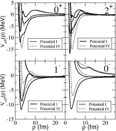
Figure 1: Three lowest Adiabatic effective potentials for the 0⁺, 2⁺, and $1^{-}$ states in ¹²Be. Results using the neutron-core potentials $I$ (solid curves) and $IV$ (dashed curves) are shown.

IV.2 Three-body energy spectrum

After solving the coupled set of radial equations (Eq.(3)) we obtain a series of ¹²Be bound states whose two-neutron separation energies are given in table 7. Columns 2 to 5 show the results obtained with the ¹⁰Be-neutron interactions given in table 1. The gaussian neutron-neutron potential is used. In order to test the role played by the short-distance details of the nucleon-nucleon interaction, we give in the sixth column the spectrum obtained when potential $I$ is combined with the Argonne $v_{8}$ neutron-neutron interaction. The last column gives the available experimental values. These results correspond to calculations without fine tuning the effective three-body potentials with a three-body force ($V_{3b}(\rho)$=0 in Eq.(3)).

Table 7: Spectrum of ¹²Be for the different neutron-core interactions (see table 1). The numerical results have been obtained without inclusion of a three-body potential in Eq.(3). In the sixth column potential $I$ has been used together with the $v_{8}$-Argonne nucleon-nucleon interaction. The energies are given in MeV.

	$W_{I}$	$W_{II}$	$W_{III}$	$W_{IV}$	$W_{I+v_{8}}$	Exper.
$0^{+}_{1}$	$-3.60$	$-3.22$	$-3.64$	$-3.77$	$-3.53$	$-3.67^{(a)}$
$2^{+}$	$-0.54$	$-0.36$	$-0.66$	$-0.96$	$-0.58$	$-1.56\pm 0.01^{(b)}$
$0^{+}_{2}$	$-0.62$	$-0.64$	$-0.64$	$-0.61$	$-0.74$	$-1.43\pm 0.02^{(c)}$
$1^{-}$	$-0.97$	$-0.97$	$-0.97$	$-1.23$	$-1.12$	$-0.99\pm 0.03^{(d)}$
$0^{-}$	$-0.96$	$-0.89$	$-0.96$	$-0.93$	$-1.17$	—

^(a) from ajz90 , ^(b) from alb78 , ^(c) from shi03 , ^(d) from iwa00b .

The bound states found can be understood assuming a simple extreme single particle model: The ground 0⁺ state should correspond to a configuration where the two neutrons occupy the two $s_{1/2}$ single-neutron states. The $1^{-}$ and the $0^{-}$ can be understood as one neutron in the $s_{1/2}$ wave and the other one in a $p_{1/2}$ state. The 2⁺ state appears with one neutron in the $s_{1/2}$ wave and the second in the $d_{5/2}$ state, and finally, the second $0^{+}$ state corresponds to both neutrons in $p_{1/2}$-waves.

For the 0${}^{+}_{1}$ ground state all the computed energies are similar, except for potential $II$, that is clearly less bound than the rest. In potential $II$ the $s$-wave neutron-core potential employed a larger range (see table 1). Since the structure of the $0_{1}^{+}$ state is expected to be dominated by the $s$-wave components, an increase of the range for this wave increases the spatial extension of the system and subsequently decreases the binding energy. In potential $IV$ the $s$-wave interaction has been constructed in a completely independent way compared to potentials $I$, $II$, and $III$. The fact that in this case the binding energy of the ground state is similar (actually slightly more bound) than for potentials $I$ and $III$, indicates that a range of 3.5 fm for the $s$-wave interaction could be more appropriate.

The $p$-wave potential is identical for the cases $I$, $II$, and $III$. Potential $IV$ also uses the same $p_{1/2}$ interaction, but different $p_{3/2}$, which however is expected to play a minor role due to the Pauli principle. This explains why the energy of the $0_{2}^{+}$ state is very much the same for all neutron-core potentials, since this state should be dominated by a $pp$ configuration.

For the 1^- (or $0^{-}$) and $2^{+}$ states a neutron in the $s_{1/2}$ wave is combined with the second neutron either in the $p_{1/2}$ or the $d_{5/2}$ state, respectively. These states are less bound than the ground state. The effect of this is more important than the confining effects of the $p$ and $d$ centrifugal barriers, and consequently the 1^- (or $0^{-}$) and $2^{+}$ states are more extended than the ground state. Therefore the effect of the larger range in potential $II$ for the $s$-wave interaction should be smaller. Actually, the 1^- energy is the same for all the three potentials. Only potential $III$, for which the $d_{3/2}$ wave was modified, produces a slightly more bound 2⁺ state.

In potential $IV$ the $d$-wave interaction is the same as in potential $I$. Also the $s$-wave and $p$-wave potentials, although obtained in a completely different way, produce similar $0^{+}$ states. However, the 1^- state, and especially the $2^{+}$ state, are more bound than with potential $I$. This indicates that the $sp$ and $sd$ interferences for these states differ between potentials $IV$ and $I$. When the gaussian neutron-neutron interaction is substituted by the $v_{8}$-Argonne potential (sixth column in table 7) similar results are found. Only a little more binding is found for the $1^{-}$, $0^{-}$ and $0^{+}_{2}$ states.

In summary, the energies obtained with the different potentials are quite stable, and the small differences found for some of the cases are insignificant, especially when taking into account the level of accuracy of the calculations at this stage. In fact, when compared to the experimental energies (last column of table 7) we see that in some cases the computed energy really disagrees with the experimental value, and even the ordering of the levels does not agree with the experiment. However, the ordering of the computed levels agrees with the extreme single particle model. The ground state should be the one having the two neutrons in the deepest single neutron level (the 0${}^{+}_{1}$ state having both neutrons in the $s_{1/2}$-wave). The first excited state should appear when one neutron jumps into the next single neutron level (the $1^{-}$ or the $0^{-}$ state having one neutron in the $s_{1/2}$-wave and the other one in the $p_{1/2}$-wave). Finally, the states corresponding to the $p_{1/2}-p_{1/2}$ and the $s_{1/2}-d_{5/2}$ configurations (0${}^{+}_{2}$ and 2⁺ states) should in principle be less bound than the $1^{-}$ and the $0^{-}$ states.

IV.3 Angular momentum decomposition

It is important to keep in mind that part of the contributions arising from core deformation have been effectively taken into account by fitting the parameters in the two-body potentials to the ¹¹Be data. In this sense, the different states found in the ¹²Be spectrum are sensitive to such deformation. However, with such two-body interactions and the core treated as an inert particle, the additional contributions arising from the $2^{+}$ excited state in ¹⁰Be are expected to play a minor role for both the $0^{+}_{1}$ and $1^{-}$ states. For the ground state because two neutrons in the $s_{1/2}$-shell and a core in a $2^{+}$ state can not produce total angular momentum zero. For the 1^- state because, although a core in a 2⁺ state and the two neutrons in the $s_{1/2}-p_{1/2}$ configuration can produce a total angular momentum 1, this structure is obviously less favorable energetically than with the core in the ground state. However, for the 2⁺ state it could be energetically efficient to excite the core into the 2⁺ state and get some extra binding by placing the two neutrons in a $s_{1/2}-s_{1/2}$ configuration. The same could happen for the second $0^{+}$ state, that could find it favorable to excite the core into the 2⁺ state and place the neutrons in the $s_{1/2}-d_{5/2}$ configuration. Therefore, the disagreement between the computed and experimental binding energies of the $2^{+}$ and $0^{+}_{2}$ states can be a signal of the importance of core excitations for these two particular states.

In any case, the deviations between computed and experimental energies are quite common when three-body calculations are performed with bare two-body interactions. All those effects going beyond the two-body correlations have obviously not been considered in the calculations. Among them are those arising from contributions of core deformation and/or core excitation. The usual cure for this problem is including an effective three-body potential ($V_{3b}(\rho)$) that simulates the neglected effects. Since these effects should appear when all the three particles are close to each other, the three-body potential should be of short-range character.

In our calculations we have used a gaussian three-body force, whose range has been taken equal to 4.25 fm, that is the hyperradius corresponding to a ¹⁰Be-core and two neutrons touching each other. The strength of the gaussian is adjusted to match the experimental energies given in the last column of table 7.

Since the $0^{-}$-state is unknown experimentally, we can not use its energy to adjust the strength of the three body force. However, in this case we expect the three-body correction to be unimportant due to the similarity of the $0^{-}$ state to the composition of the $1^{-}$-state where the experimental energy is reproduced without any three-body force. This indicates that the computed $0^{-}$-energy also is close to the correct value.

Including the three-body potentials we have the four potentials specified in table 1, and in addition potential $I$ combined with the $v_{8}$-Argonne neutron-neutron potential. We then arrive at the contributions of the different partial wave components given in the last five columns of tables 3 to 6 for the 0⁺, $2^{+}$, $0^{-}$ and $1^{-}$ states. The dominating components are in all the cases as expected from the extreme single particle picture. When the three-body wave functions are written in the second or third Jacobi set ($\bm{x}$ from core to neutron, lower part of the tables) the dominating components are the $\ell_{x}$=$\ell_{y}$=0 ($\sim 70\%$) for the $0^{+}_{1}$ ground state, the $\ell_{x}$=$\ell_{y}$=1 ($\sim 75\%$) for the $0^{+}_{2}$ state, the $\{\ell_{x}$=0,$\ell_{y}$=$2\}$ and $\{\ell_{x}$=2,$\ell_{y}$=$0\}$ components ($\sim 90\%$ in total) for the $2^{+}$ state, and the $\{\ell_{x}$=0,$\ell_{y}$=$1\}$ and $\{\ell_{x}$=1,$\ell_{y}$=$0\}$ components ($\sim 98\%$ and $\sim 99\%$ in total) for the $1^{-}$ and $0^{-}$ states. Although the precise numbers can change a little from one potential to another, the differences are not significant. The residual contributions are more relevant for the $0^{+}$ states. The ground state has a $p$-wave contribution of about 13% to 19%, and a $d$-wave contribution of about 10% to 13%. The second $0^{+}$ state has an $s$-wave contribution from 15% to 23%, and a $d$-wave contribution from 6% to 8%.

In nav00 the configuration with the two outer neutrons in the $p$-shell for the 0⁺ ground state amounts to 32% of the wave function, which is clearly larger than the 13%-19% obtained in this work. In bar77 this value is given to range between 20% and 40%. Correspondingly, the contribution from configurations with the two neutrons in the $sd$-shell is larger in our calculation than in nav00 ; bar77 . In these two references the individual contributions from $s$ and $d$-waves are not given. In general, for both ¹¹Li and ¹²Be the $s$-wave components are larger in cluster models than in shell model calculations. One reason for ¹²Be is that the $d$-waves are underestimated in the cluster model due to the neglect of the core-excited $2^{+}$ state. Another reason could be that large spatial extension is harder to describe in shell models than in cluster models. Since $s$-waves for a given energy extend to larger distances than $d$-waves the shell model tend to underestimate the $s$-wave components. As we shall show later the contributions obtained in the present work are consistent with the measured invariant mass spectrum given in pai06 .

Table 8: Root mean square radii (in fm) for the different bound states in ¹²Be with the four neutron-core interactions. A gaussian three-body forced is included to fit the experimental binding energies. The range of the three-body force is 4.25 fm. Sixth column is as potential $I$ + $v_{8}$ Argonne nucleon-nucleon interaction.

	$W_{I}$	$W_{II}$	$W_{III}$	$W_{IV}$	$W_{I+v_{8}}$	Exper.
$0^{+}_{1}$	2.60	2.63	2.60	2.61	2.60	$2.59\pm 0.06^{(a)}$
$2^{+}$	2.72	2.74	2.68	2.70	2.67	—
$0^{+}_{2}$	2.88	2.91	2.87	2.90	2.87	—
$1^{-}$	3.23	3.24	3.23	3.19	3.16	—
$0^{-}$	3.18	3.35	3.18	3.18	3.00	—

^(a) from tan88

IV.4 Wave functions

The rms radii for the computed bound states are given in table 8. The results are essentially independent of the core-neutron potential used. The only available experimental value is the one corresponding to the $0^{+}_{1}$ ground state tan88 , for which a good agreement between theory and experiment is found.

Table 9: For the different computed states in ¹²Be, and the different neutron-core potentials, root mean square distances (in fm) $\langle r_{nn}\rangle^{1/2}$ and $\langle r_{cn}\rangle^{1/2}$, where $n$ and $c$ denote an external neutron and the core, respectively. A gaussian three-body force is included to fit the experimental binding energies.

		$W_{I}$	$W_{II}$	$W_{III}$	$W_{IV}$	$W_{I+v_{8}}$
$0^{+}_{1}$	$\langle r^{2}_{nn}\rangle^{1/2}$	4.5	4.6	4.4	4.3	4.4
	$\langle r^{2}_{cn}\rangle^{1/2}$	4.0	4.1	4.0	4.1	4.0
$2^{+}$	$\langle r^{2}_{nn}\rangle^{1/2}$	5.7	5.8	5.4	5.2	5.4
	$\langle r^{2}_{cn}\rangle^{1/2}$	4.4	4.5	4.3	4.4	4.3
$0^{+}_{2}$	$\langle r^{2}_{nn}\rangle^{1/2}$	7.3	7.8	7.3	7.7	7.3
	$\langle r^{2}_{cn}\rangle^{1/2}$	5.0	5.1	5.0	5.1	5.0
$1^{-}$	$\langle r^{2}_{nn}\rangle^{1/2}$	8.8	9.2	8.7	8.1	8.3
	$\langle r^{2}_{cn}\rangle^{1/2}$	6.4	6.7	6.4	6.1	6.0
$0^{-}$	$\langle r^{2}_{nn}\rangle^{1/2}$	9.2	9.9	9.2	9.2	8.4
	$\langle r^{2}_{cn}\rangle^{1/2}$	6.0	6.4	5.9	6.0	5.4

Figure 2: Contour diagram for the probability distribution of 0${}^{+}_{1}$ state in ¹²Be. The square of the three-body wave function is integrated over the directions of the two Jacobi coordinates.

Figure 3: The same as Fig.2 for the $0^{+}_{2}$ state in ¹²Be.

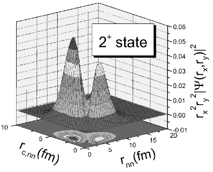
Figure 4: The same as Fig.2 for the $2^{+}$ state in ¹²Be.

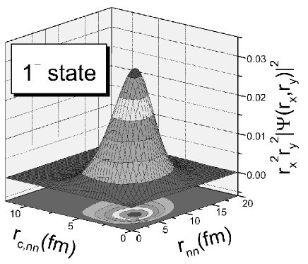
Figure 5: The same as Fig.2 for the $1^{-}$ state in ¹²Be.

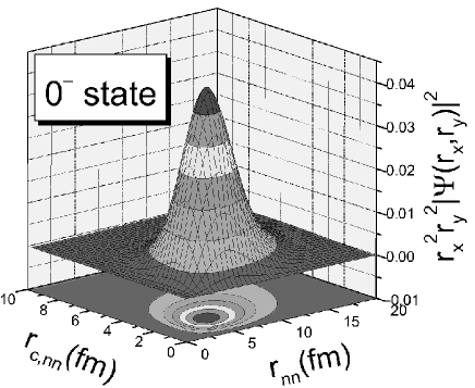
Figure 6: The same as Fig.2 for the $0^{-}$ state in ¹²Be.

The geometry of the different states is reflected in the results given in table 9, where we give the rms distances between the two neutrons ($\langle r^{2}_{nn}\rangle^{1/2}$), and between the core and one of the neutrons ($\langle r^{2}_{cn}\rangle^{1/2}$) for the different cases. The ground state corresponds mainly to the three particles placed in the vertices of an equilateral triangle. For the excited states, the smaller binding obviously implies a larger distance between particles. But, as seen in table 9, the distance between the neutrons grows clearly faster than the one between the neutron and the core. In fact, for the less bound excited states (the 1^- and $0^{-}$ states) the distance between the two neutrons is roughly a factor of two larger than the corresponding distance in the ground state, while the neutron-core distance increases by a factor of 1.5.

The spatial distribution of the three constituents can be better seen in Figures 2 to 6, where we show the probability distribution for the $0^{+}_{1}$, $0^{+}_{2}$, 2⁺, 1^- and $0^{-}$ states in ¹²Be. The probability distribution is defined as the square of the three-body wave functions multiplied by the phase space factors and integrated over the directions of the two Jacobi coordinates. In particular, in the figures we have chosen the first Jacobi set, such that the distributions are plotted as function of the distance between the two neutrons ($r_{nn}$) and the distance between the core and the center of mass of the two neutrons ($r_{c,nn}$), respectively. The $0^{+}_{1}$ and the $2^{+}$ states have the largest probabilities when the two neutrons are separated from each other almost the same distance as from the core (about 2.2 fm and 2.6 fm, respectively). On the other hand, $0^{+}_{2}$, $0^{-}$ and $1^{-}$ states have the largest probabilities when the two neutron are well separated from each other (about 5.5 fm) while they are closer to the core (about 3.5 fm). The $2^{+}$ state has also a secondary probability maximum with this last geometry.

V Transition strengths

The bound states can only decay electromagnetically. The corresponding observable transition probabilities are critically depending on the structures. Thus they provide experimental tests and we therefore compute the lifetimes for future comparison. The selection rules determine the dominating transitions which can be of both electric and magnetic origin.

V.1 Electric transitions

The electric multiple operators are defined as:

$${\cal M}_{\mu}(E\lambda)=e\sum_{i=1}^{A}Z_{i}r_{i}^{\lambda}Y_{\lambda,\mu}(\hat{r}_{i})$$ (6)

where $A$ is the number of constituents in the system, each of them with charge $eZ_{i}$, and where $\bm{r}_{i}$ is the coordinate of each of them relative to the $A$-body center of mass.

The electric multipole strength functions are defined as:

$${\cal B}(E\lambda,I_{i}\rightarrow I_{f}) = \sum_{\mu M_{f}}|\langle I_{f}M_{f}|{\cal M}_{\mu}(E\lambda)|I_{i}M_{i}\rangle|^{2}$$ (7)

$$= \frac{1}{2I_{i}+1}|\langle I_{f}||{\cal M}(E\lambda)||I_{i}\rangle|^{2}$$

Also, following shi07 , we consider the monopole transition operator:

$${\cal M}_{0}(E0)=e\sum_{i=1}^{A}Z_{i}r_{i}^{2}$$ (8)

In our three-body model, where $A-2$ constituents are assumed to form a well defined core, the operators (6) and (8) contain one term directly associated to the three-body system having the form:

$${\cal M}_{\mu}(E\lambda) = e\sum_{i=1}^{3}Z_{i}r_{i}^{\lambda}Y_{\lambda,\mu}(\hat{r}_{i})$$ (9)

$${\cal M}_{0}(E0) = e\sum_{i=1}^{3}Z_{i}r_{i}^{2}$$ (10)

where $i$ labels the three constituents. In addition to Eqs.(9) and (10) there is a contribution from the intrinsic core multipole operators. In particular, for the electric dipole and quadrupole operators the precise expressions are given by Eqs.(21) and (A). For the quadrupole case, Eq.(A), there is an additional contribution arising from the coupling between the electric dipole operator of the core and its motion around the three-body center-of-mass.

When an inert core has spin zero, as in the present ¹²Be model, the contributions from the intrinsic core multipole operators ${\cal M}_{\mu}(E\lambda,core)$ are zero. These terms contribute only when core excitations are included. For ¹²Be the first excited state of the ¹⁰Be-core is a 2⁺ state at about 3.4 MeV. Its effect on the ${\cal B}(E1)$ strength must be small, since the ${\cal M}_{\mu}(E1,core)$ operator does not couple the $0^{+}$ and $2^{+}$ core states. Therefore the ${\cal B}(E1)$ strength is expected to be less dependent on the contribution of the 2⁺ excited state in the core than the ${\cal B}(E2)$ strength, where the ${\cal M}_{\mu}(E2,core)$ operator does couple the $0^{+}$ and $2^{+}$ states in the core.

Also, the ${\cal M}_{0}(E0,core)$ operator is not coupling the $0^{+}$ and $2^{+}$ states of the core. However, the expectation value of this operator between the 0⁺ ground state of the core is not zero (it is actually related to the rms radius of the core). Nevertheless, for an inert core with spin zero, the total nuclear wave function factorizes into the three-body cluster wave function and the core wave function. In this way, the expectation value of ${\cal M}_{0}(E0,core)$ between wave functions corresponding to different states is automatically zero due to the orthogonality of the three-body cluster wave functions.

For ¹¹Be (¹⁰Be+$n$) the experimental value of the ${\cal B}(E1,\frac{1}{2}^{-}\rightarrow\frac{1}{2}^{+})$ transition strength is $0.115\pm 0.010$ e² fm² mil83 . Direct application of Eq.(9) assuming zero charge for the neutrons fails in reproducing this value. However, it is well known that to take into account the distortion or polarization of the core one has to include an effective charge for the neutrons suz04 ; hor06 . Due to the square in Eq.(7) two different neutron effective charges are found to fit the experimental value for ${\cal B}(E1,\frac{1}{2}^{-}\rightarrow\frac{1}{2}^{+})$: $Z_{n}=0.28$ and $Z_{n}=0.52$. These two charges give rise to slightly different mean square charge radii for the ground state in ¹¹Be of about 2.7 fm and 3.0 fm, respectively. The ¹⁰Be-neutron potential only has marginal effect and only 2.7 fm is consistent with the experimental value of 2.63$\pm$0.05 fm tan88 . Therefore a neutron effective charge of $Z_{n}$=0.28 has been used in the following calculations.

Table 10: ${\cal B}(E1)$ (in e² fm²), ${\cal B}(E2)$ (in e² fm⁴) transition strengths between the computed states in ¹²Be given in table 7 and ${\cal M}(E0)$ (in e fm²) between the two 0⁺ states. An effective three-body force has been used to fit the experimental binding energies.

	$W_{I}$	$W_{II}$	$W_{III}$	$W_{IV}$	$W_{I+v_{8}}$	Exper.
${\cal B}(E1,0_{1}^{+}\rightarrow 1^{-})$	0.046	0.052	0.048	0.064	0.051	$0.051\pm 0.013^{(a)}$
${\cal B}(E1,0_{2}^{+}\rightarrow 1^{-})$	0.016	0.006	0.016	0.010	0.015	—
${\cal B}(E1,2^{+}\rightarrow 1^{-})$	0.0054	0.0074	0.0079	0.018	0.0081	—
${\cal B}(E2,2^{+}\rightarrow 0_{1}^{+})$	3.14	3.50	3.52	3.93	3.04	$5.5-8.2^{(b)}$
${\cal B}(E2,2^{+}\rightarrow 0_{2}^{+})$	0.024	0.32	0.044	0.12	0.047	$1.40\pm 0.12^{(c)}$
${\cal M}(E0,0_{2}^{+}\rightarrow 0_{1}^{+})$	1.89	0.60	1.77	1.13	1.99	$0.87\pm 0.03^{(c)}$

^(a) from iwa00b ,^(b) estimation from experimental data in iwa00 ,^(c) from shi07

In table 10 we give the computed ${\cal B}(E\lambda)$ values for transitions between the states in table 7 and the monopole transition matrix element ${\cal M}(E0)\equiv|\langle 0^{+}_{2}|{\cal M}_{0}(E0)|0^{+}_{1}\rangle|$. An effective three-body force has been included to fit the experimental binding energies for the different ¹²Be states. The results are quite stable for the different neutron-core potentials used. The only exception are the transitions in which the $0^{+}_{2}$ state is involved. This state is the one showing the most important dependence on the potential used. In particular potentials $II$ and $IV$ produce an $s$-wave content (lower part of table 3) about 50% larger than potentials $I$ and $III$. As seen in the table the results are sensible to this difference, since the values found for ${\cal B}(E2,2^{+}\rightarrow 0_{2}^{+})$, ${\cal B}(E1,0^{+}_{2}\rightarrow 1^{-})$ and ${\cal M}(E0)$ with potentials $II$ and $IV$ clearly differ from the ones with $I$ and $III$.

For the ${\cal B}(E1)$ transitions, the experimental value of $0.051\pm 0.013$ e² fm² corresponding to the $0_{1}^{+}\rightarrow 1^{-}$ transition iwa00b , agrees well with the results given in the first row of table 10. The agreement is equally good for all the neutron-core potentials used. Only for potential $IV$ the computed value is a bit higher compared to the other cases, but the computed result is still lying within the experimental error. Therefore the three-body model used reproduces well the experimental value, although it is worth emphasizing that the effective neutron charge also is introduced to simulate neglected effects of core deformation and polarization. The small effect from the three-body potential can be attributed to the choice of minimal structure, which means no dependence on angular momentum quantum numbers. The only essential effect is an adjustment of the three-body energy which in turn may have an effect on the spatial extension, but leaving all structures unchanged. For the other two $E1$ transitions experimental data are not available.

Using the same effective neutron charge we get the ${\cal B}(E2)$ values in the central part of table 10. Assuming that the $2^{+}$ state in ¹²Be is a rotational state built on the ground state, an experimental value of $2.00\pm 0.23$ is given in iwa00 for the deformation length $\delta$ in ¹²Be. This assumption means that the ${\cal B}(E2,2^{+}\rightarrow 0^{+}_{1})$ value is given by $\frac{1}{5}\left(\frac{3}{4\pi}Ze\delta\right)^{2}R^{2}$, which equals $5.5\pm 1.3$ e² fm⁴ or $8.2\pm 1.9$ e² fm⁴ for $R\approx 1.2A^{1/3}$ fm or $R=\sqrt{5/3}\langle r^{2}\rangle^{1/2}$, respectively. Here $\langle r^{2}\rangle^{1/2}$ is the experimental charge r.m.s. radius of ¹²Be. Both values are higher than obtained numerically (first line in the central part of the table).

Also the recently measured value of $1.40\pm 0.12$ e² fm⁴ shi07 for ${\cal B}(E2,2^{+}\rightarrow 0^{+}_{2})$ is much larger than all the computed results in the table, which varies about one order of magnitude with the different neutron-core potentials. Furthermore we see that the computed ${\cal B}(E2,2^{+}\rightarrow 0^{+}_{1})$ is much larger than ${\cal B}(E2,2^{+}\rightarrow 0^{+}_{2})$. This arises from the fact that the $2^{+}$ state is dominated by the $sd$ interferences in the second and third Jacobi sets (lower part of table 4), while the $0_{2}^{+}$ state is dominated by a $pp$ configuration (lower part of table 3). When the core is infinitely heavy these dominating configurations must give a vanishing contribution from Eq.(9) to the ${\cal B}(E2,2^{+}\rightarrow 0^{+}_{2})$ value. Thus, the values in table 10 have to be small and very sensitive to the non-dominating components in the two states.

Small variations in the contribution of some of these smaller components can produce large relative changes in the computed transition strength. In particular, for the $0_{2}^{+}$ state, the $\ell_{x}=1$ components clearly dominate but a substantial probability appears in the $\{\ell_{x}=0,S=0\}$ component, which coincides with a large probability for the $\{\ell_{x}=0,S=0\}$ component in the $2^{+}$ state, see the lower part of table 4. For potentials $II$ and $IV$ this $s$-wave component in the $0^{+}_{2}$ state (table 3) is significantly larger than for the other three potentials. This implies a larger overlap, and therefore a larger ${\cal B}(E2)$ transition strength.

At this point it is important to emphasize that the computed results are obtained for an inert core. For $E2$-transitions a non-negligible contribution from the $2^{+}$ excited state in the ¹⁰Be-core is expected. The second term in the electric quadrupole operator (A), together with the existence of the core excited $2^{+}$-state, give rise to another non-vanishing contribution. In fact, for ¹⁰Be the experimental ${\cal B}(E2,2^{+}\rightarrow 0^{+})$ transition strength is known to be 10.4 e² fm⁴ ram87 . Thus the computed three-body ${\cal B}(E2)$ values should be supplemented by the contribution of 10.4 e² fm⁴ multiplied by the weight factor corresponding to the admixtures of the $2^{+}$ core excitation in the ¹²Be states. In fact, this contribution should provide most of the strength for the $2^{+}\rightarrow 0^{+}_{2}$ transition. In contrast, the contribution from the last term in the quadrupole transition operator (A) is expected to be small, since ${\cal M}_{\mu}(E1,core)$ cannot couple $0^{+}$ and $2^{+}$ states.

In shi07 an experimental value of $0.87\pm 0.03~{}$e fm² is given for the monopole transition matrix element between the two $0^{+}$ states. This observable gives information about the relative structures of the these two states. The computed results are given in the last row of table 10, and they are clearly higher (except for potential $II$) than the experimental value, but similar to the value of $1.7$ e fm² obtained in Ref. kan03 . However, as seen in the table, the computed results are very sensitive to the contribution of the relative neutron-¹⁰Be $s$-wave. An increase from about 15% to 23% reduces the computed ${\cal M}(E0)$ by a factor of 3 (going in fact through the experimental value). This $s$-wave contribution could easily change significantly when core excitations are included in the $0_{2}^{+}$ wave function, for which, as mentioned at the beginning of subsection IV.3, such excitations could play a relevant role.

V.2 Magnetic transitions

For the unobserved predicted $0^{-}$ state the dominating multipolarities for its possible decays are of magnetic character. Only $M1$ and $M2$ transitions to the $1^{-}$ or the $2^{+}$ states are possible.

The magnetic multiple operator is defined as:

$${\cal M}_{\mu}(M\lambda)=\frac{e\hbar}{2Mc}\sqrt{\lambda(2\lambda+1)}\sum_{i}r_{i}^{\lambda-1}$$ (11)

$$\left[\left(g_{s}^{(i)}-\frac{2g_{\ell}^{(i)}}{\lambda+1}\right)(Y_{\lambda-1}s)+\frac{2g_{\ell}^{(i)}}{\lambda+1}(Y_{\lambda-1}j)\right]_{(\lambda-1,1)\lambda\mu}$$

where the constants $g_{s}$ and $g_{\ell}$ depend on the constituent particles $i$. The magnetic multipole strength functions are defined as for the electric case (see Eq.(7)).

In particular, the ${\cal M}1$ and ${\cal M}2$ operators involved in the magnetic dipole and quadrupole decay of the $0^{-}$ state into the $1^{-}$ and $2^{+}$ states are

$${\cal M}_{\mu}(M1) = \frac{e\hbar}{2Mc}\sqrt{\frac{3}{4\pi}}\sum_{i}(g^{(i)}_{s}\vec{s}_{i}+g^{(i)}_{\ell}\vec{\ell}_{i})_{\mu}$$ (12)

$${\cal M}_{\mu}(M2) = \frac{e\hbar}{Mc}{\frac{5}{\sqrt{2}}}\sum_{i}\sum_{\nu,q}\left(\begin{array}[]{ccc}1&1&2\\ \nu&q&-\mu\end{array}\right)Y_{1,\nu}(\Omega_{i})$$ (16)

$$\left(g^{(i)}_{s}\vec{s}_{i}+\frac{2g^{(i)}_{\ell}}{3}\vec{\ell}_{i}\right)_{q}\;,$$

where $q$ labels the spherical component of an operator.

We can identify a source of uncertainties in the transition strength estimates, which comes from the effective values of the g-factor in these expressions.

The core has angular momentum zero and therefore a vanishing effective spin $g_{s}^{(c)}$-factor and $g_{\ell}^{(c)}$= 4. We also use the free value of $g_{s}^{(n)}$=$-3.82$ and we use again an effective neutron charge $g_{\ell}^{(n)}$=$0.28$. The transition operators are then defined and we can compute the ${\cal B}(M1,0^{-}\rightarrow 1^{-})$ and ${\cal B}(M2,0^{-}\rightarrow 2^{+})$ transition strengths. The results are given in table  11, where we observe that the computed values are rather independent of the particular neutron-core potential used. Only for potential $IV$ the results deviate by up to factor of two from the other estimates. This is reflecting the fact that potential $IV$ is producing a different distribution of the weights between the components in the $1^{-}$ and $2^{+}$ states (see tables 6 and 4).

As mentioned above, the effective values of the $g$-factors are rather uncertain and spin polarization could reduce $g_{s}$ by a factor of 2, change $g_{\ell}^{(c)}$ by perhaps 10 %, and vary $g_{\ell}^{(n)}$ from the assumed effective value (see also the discussion of the empirical evidence in boh69 ). As discussed in rom07 , the computed magnetic strength has a very limited dependence on the precise values used for the orbital gyromagnetic factors $g_{\ell}$, and they are mainly only sensitive to $g_{s}^{(n)}$. In particular, use of $g_{s}^{(n)}$=$-2.0$ reduces the computed magnetic strengths by a factor of about 3.

In summary, the decay possibilities for the $0^{-}$ state are limited to magnetic transitions. Even with fairly reliable estimates for the transition probabilities it is not easy to give an accurate prediction for the lifetime of this state. If $0^{-}$ is below the $1^{-}$ state only decay into $2^{+}$ is possible and the resulting lifetime can be estimated to be of the order $10^{-8}$ sec. However, if $0^{-}$ can decay into the $1^{-}$ state the possibly very small energy difference causes a large uncertainty which could reduce the lifetime to about $10^{-11}$ sec or perhaps even somewhat smaller. In any case these estimates justify the classification of this new $0^{-}$ state as an isomer in ¹²Be.

Table 11: ${\cal B}(M1)$ (in e² fm²) and ${\cal B}(M2)$ (in e² fm⁴) transition strengths between the computed states in ¹²Be given in table 7. An effective three-body force has been used to fit the experimental binding energies.

	$W_{I}$	$W_{II}$	$W_{III}$	$W_{IV}$	$W_{I+v_{8}}$
${\cal B}(M1,0^{-}\rightarrow 1^{-})$	0.060	0.061	0.059	0.049	0.061
${\cal B}(M2,0^{-}\rightarrow 2^{+})$	0.94	0.78	0.78	0.43	0.85

VI Invariant mass spectrum

One of the tools for studying the structure of three-body halo nuclei was breakup reactions on a target. By relatively fast removal of one of the constituents the remaining two are essentially left undisturbed and measurements of their momenta then provide fairly direct information about the initial state. We use this technique to investigate the two-body substructures of ¹²Be. The experimental relative ¹⁰Be-neutron energy spectrum (or invariant mass spectrum) after ¹²Be breakup on a carbon target at a beam energy of 39.3 MeV/nucleon is shown in ref.pai06 . Both fragments, ¹⁰Be and neutron, are simultaneously detected, and their relative decay energy is reconstructed from the measured momenta. The final ¹⁰Be-neutron states are then restricted to unbound states in ¹¹Be.

This spectrum can easily be computed by use of the sudden approximation. We assume that the target transfers a (relatively large) momentum to one of the particles (one of the neutrons) in the projectile which then is instantaneously removed. The remaining two particles, the ¹⁰Be-core and the second neutron, are just spectators in the reaction, meaning that they continue their motion undisturbed without further interaction with the removed particle. They do, however, continue to interact with each other.

Under this assumption the differential cross section of the process takes the form:

$$\frac{d^{6}\sigma}{d\bm{k}_{x}d\bm{k}_{y}}\propto\sum_{M}\sum_{s_{x}\sigma_{x}\sigma_{y}}\left|\langle e^{i\scriptsize\bm{k}_{y}\cdot\scriptsize\bm{y}}\chi_{s_{y}}^{\sigma_{y}}w_{s_{x}}^{\sigma_{x}}(\bm{k}_{x},\bm{x})|\Psi^{JM}(\bm{x},\bm{y})\rangle\right|^{2}$$ (17)

where $\Psi^{JM}$ is the three-body wave function with total angular momentum $J$ and projection $M$, $\bm{k}_{x}$ and $\bm{k}_{y}$ are the momenta associated to the Jacobi coordinates $\bm{x}$ and $\bm{y}$, $s_{x}$ and $s_{y}$ are the coupled spin of the spectator two-body system and the spin of the removed particle, respectively, and $\sigma_{x}$ and $\sigma_{y}$ are the corresponding spin projections. Finally, $w_{s_{x}}^{\sigma_{x}}$ is the continuum two-body wave function of the spectators (¹⁰Be and neutron) in the final state. This two-body wave function is computed with the corresponding two-body interaction and the boundary condition at small distance determined to be precisely the ¹⁰Be-neutron structure left by removing the other neutron in ¹²Be, see gar97b for a detailed description.

After integration of Eq.(17) over $\bm{k}_{y}$ and the angles describing the direction of $\bm{k}_{x}$ we obtain the differential cross section $d\sigma/dk_{x}$, which is related to the invariant mass spectrum as shown in gar97 :

$$\frac{d\sigma}{dE_{nc}}=\frac{E_{c}E_{n}}{E_{c}+E_{n}}\frac{m(M_{c}+M_{n})}{M_{c}M_{n}}\frac{1}{k_{x}}\frac{d\sigma}{dk_{x}}$$ (18)

where $E_{c}$ and $M_{c}$ are the core energy and mass, $E_{n}$ and $M_{n}$ the neutron energy and mass, $E_{nc}$ the relative neutron-core energy, and $m$ is the normalization mass used to define the Jacobi coordinates.

The presence in Eq.(17) of the two-body wave function $w_{s_{x}}^{\sigma_{x}}(\bm{k}_{x},\bm{x})$ makes it evident that the invariant mass spectrum (18) crucially depends on the final state two-body interaction. It is important to note that Eq.(17) is not assuming that the two spectators populate two-body resonances in the final state. The two-body wave function $w_{s_{x}}^{\sigma_{x}}$ contributes for any value of the relative two-body momentum $\bm{k}_{x}$, not only for those where $\bm{k}_{x}$ matches a two-body resonance energy. Except for those very precise values of $\bm{k}_{x}$, $w_{s_{x}}^{\sigma_{x}}$ is just an ordinary continuum two-body wave function.

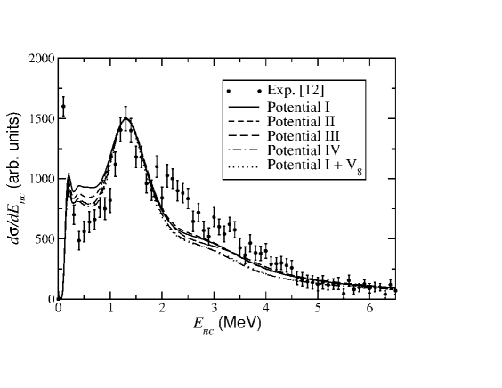
Figure 7: Relative energy spectrum of ¹⁰Be+neutron after fragmentation of ¹²Be on a light target. The solid, short-dashed, long-dashed, dot-dashed, and dotted curves correspond to calculations using potentials $I$, $II$, $III$, $IV$, and $I+v_{8}$, respectively. The experimental data correspond to fragmentation of ¹²Be on carbon at a beam energy of 39.3 MeV/nucleon pai06 .

In Fig.7 we show the relative core-neutron energy spectrum after removal of one neutron from ¹²Be on a light target according to Eq.(18). The results for the different ¹⁰Be-neutron interactions used in this work are shown. The computed curves have been scaled to the experimental data pai06 . Also, the experimental energy resolution has been taken into account by convoluting the computed distributions with a gaussian having a full width at half maximum (FWHM) equal to $0.4E^{1/2}$ ($E$ in MeV) pai06 .

As a general result, all the potentials reproduce equally well the peak at about 1.2 MeV, and the tail of the distribution. In the same way all of them underestimate the spectrum in the region around 2.2 MeV and do not reproduce the very narrow peak at very low energies. Potential $IV$ (dot-dashed curve) is reproducing the peak at 1.2 MeV best of all, but on the other hand gives a worse agreement with the experiment in the region between 3 and 4 MeV. Compared to the results with potential $I$ (solid curve), inclusion of the Argonne nucleon-nucleon potential (dotted curve) slightly improves the behaviour at small energies but also slightly spoils the agreement with the experiment at large energies.

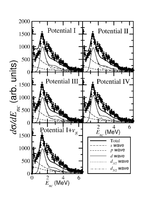
Figure 8: Relative energy spectrum of ¹⁰Be+neutron after fragmentation of ¹²Be on a light target (thick solid curve), and the contributions to it from $s$-waves (long-dashed), $p$-waves (short-dashed), and $d$-waves (thin solid). The $d$-wave contribution is split into the $d_{3/2}$ contribution (dotted) and the $d_{5/2}$ contribution (dot-dashed). The different panels show the spectra corresponding to the potentials in table 1 and the case with potential $I$ plus the Argonne $v_{8}$ nucleon-nucleon potential. Experimental data from pai06 .

In Fig.8 we show, for different ¹⁰Be-neutron potentials, the contribution from $s$-, $p$-, and $d$- waves to the total invariant mass spectrum. Here $s$, $p$, and $d$ refer to the value of the ¹⁰Be-neutron relative orbital angular momentum. In the figure the dotted and dot-dashed curves give the contribution from the $d_{3/2}$ and $d_{5/2}$-waves, respectively. We notice that the main peak in the distribution is produced by the $d_{5/2}$-wave. This can be traced back to the $5/2^{+}$ resonance in ¹¹Be at 1.28 MeV above threshold. The 3/2⁺ resonance, with an energy of 2.90 MeV, helps to match the experimental tail of the distribution. The $s$- and $p$-waves contribute mainly at small energies, and they are almost entirely responsible for the distribution below 1 MeV.

From Fig.8 it is now easy to understand that the main disagreement between the computed curves and the experimental data is due to the absence in the calculation of the 3/2^- resonance in ¹¹Be, whose energy above threshold is 2.19 MeV, precisely the energy region where the disagreement is found. However, as already mentioned, inclusion of this resonance necessarily requires information beyond the present ¹²Be three-body model with an inert ¹⁰Be core. If we still insist on the picture of a three-body system with a ¹⁰Be core, then a 3/2^- state in ¹¹Be needs either a neutron in the $p$-shell coupled to the 2⁺ state of ¹⁰Be, or a neutron in the $sd$-shell coupled to ¹⁰Be in a negative parity state. Another possibility is of course to use a different cluster description for ¹²Be, like for instance ⁹Be in the 3/2^- ground state plus three neutrons. Therefore, except for the lack of this state in the ¹¹Be spectrum, the contributions obtained in this work for the 0⁺ ground state are consistent with the experimental invariant mass spectrum given in pai06 .

The highest ¹¹Be resonance that has been considered in our calculations is the $3/2^{+}$ state at 2.90 MeV. The next excited states in ¹¹Be are the $5/2^{-}$ and $3/2^{-}$ resonances with energies above threshold at 3.49 MeV and 3.46 MeV, respectively hir05 . For the same reason as the $3/2^{-}$ state at 2.19 MeV, these two states can not be included in our three-body picture with an inert ¹⁰Be core. In any case, decay of these two resonances into the ground state of ¹⁰Be plus a neutron would give some small contribution to the tail of the invariant mass spectrum. However, these two states can also decay into ¹⁰Be plus a neutron but leaving ¹⁰Be in its $2^{+}$ excited state at 3.37 MeV. Therefore very little energy is left for the neutron after such decay (less than 100 keV hir05 ), giving rise to the experimental sharp peak at very low energies. Theoretical calculation of this peak requires then also inclusion of core excitations in the model.

In zah93 the experimental FWHM of the ¹⁰Be longitudinal momentum distribution after fragmentation of ¹²Be on a carbon target (beam energy equal to 56.8 MeV/nucleon) is found to be $194\pm 9$ MeV$/c$. Within the sudden approximation, such distribution can also be computed from Eq.(17), see gar97b for details. The widths of the longitudinal core momentum distributions are computed to be 162 MeV$/c$, 159 MeV$/c$, 169 MeV$/c$, 171 MeV$/c$, and 166 MeV$/c$ for the neutron-core potentials $I$, $II$, $III$, $IV$, and $I$+$v_{8}$, respectively.

Inclusion of core excitations should help to reduce the discrepancy between the computed widths and the experimental value. The components having spin of the core equal to 2, and coupling to the total angular momentum zero of the ¹²Be ground state, must necessarily contain non-zero values for $\ell_{x}$ or/and $\ell_{y}$. This means additional centrifugal barriers which attempt to confine the three-body system to smaller spatial extension, and subsequently producing broader momentum distributions.

VII Summary and conclusions

The properties of ¹²Be have been investigated assuming a three-body structure with an inert ¹⁰Be core and two neutrons. A description of the nucleus by use of the hyperspherical adiabatic expansion method is particularly appropriate in this case, since two of the two-body subsystems have bound states. The symmetric treatment of all the two-body interactions makes it easier to reproduce the correct two-body asymptotics. This could be especially important for the weakly bound excited states.

We constructed four different neutron-¹⁰Be interactions, each of them reproducing the known spectrum of ¹¹Be up to an excitation energy of 3.41MeV. However, the 3/2^- resonance in ¹¹Be has been excluded, since it requires the ¹⁰Be core to be in an excited state. This case goes beyond the three-body model with an inert core that is used in this work. Nevertheless, part of the effects arising from core deformation are effectively taken into account through the fitting procedure of the neutron-¹⁰Be potential. For the neutron-neutron interaction two different potentials have been used, both reproducing low-energy scattering data.

We have found two $0^{+}$, one $2^{+}$, one $1^{-}$ and one $0^{-}$ bound states. The first four are known experimentally, but not the $0^{-}$ state. The computed binding energies agree reasonably well with the experimental value for the ground $0^{+}$ state and the excited $1^{-}$ state. For the second $0^{+}$ and the $2^{+}$ states a larger discrepancy is found, which can be attributed to contributions from core excitations additional to the ones masked in the neutron-¹⁰Be potential. To reproduce the experimental two-neutron separation energies for these states we included a three-body force.

The dominating components of the wave functions correspond to the ones expected from the extreme single particle model. The ratio of the computed neutron-neutron and core-neutron root mean square distances increases with the excitation energy. All possible electric and magnetic transition strengths have also been computed. An effective charge for the neutron is used to take into account distortion or polarization of the core. This effective charge has been obtained by adjusting the calculation to reproduce the experimental ${\cal B}(E1)$ transition strength in ¹¹Be, as well as its charge root mean square radius.

Core excitations can contribute to transition strengths in two different ways. There could be a direct contribution arriving from the transition between two core states or a contribution to the wave function of a ¹²Be state then leading to an indirect effect on transition strengths.

The direct contribution of core excitations in the ¹²Be monopole and dipole strength functions should be negligible, since $r^{2}$, ${\cal M}_{\mu}(E1)$ and ${\cal M}_{\mu}(M1)$ operators cannot couple the $J$=0 and $J$=2 states. On the other hand, quadrupole transition operators can couple these states and there could be an important effect from the excitation of the core. The possible contribution of core excitations to wave functions of $2^{+}$ and $0_{2}^{+}$ states could lead to some uncertainties in the calculated transition strengths involving those states. Our calculations reproduce rather well the available experimental data.

The relative ¹⁰Be-neutron energy spectrum after ¹²Be breakup on a carbon target at a beam energy of 39.3 MeV/nucleon has been computed within the sudden approximation. For all the potentials the experimental spectrum is rather well reproduced. Only in the region around 2.2 MeV the computed curves underestimate the experiment. This is due to the absence of the 3/2^- resonance in our ¹¹Be spectrum, which originates from ¹⁰Be-core excited states.

In summary, a frozen-core three-body model is able to reproduce most of the properties of ¹²Be: ground and excited bound states, electromagnetic transition strengths, and invariant mass spectrum after high-energy breakup. Core excitations, however, are needed to improve the two-neutron separation energies for the $0^{+}_{2}$ and $2^{+}$ states, to get a better estimate of the quadrupole transition strengths and monopole transition matrix element, and to fine tune the agreement with the experimental invariant mass spectrum.

ACKNOWLEDGMENTS

We are grateful to K. Riisager for drawing our attention to the problems of weakly bound excited states investigated here. This work was partly support by funds provided by DGI of MEC (Spain) under contract No. FIS2005-00640. One of us (C.R.R.) acknowledges support by a predoctoral I3P grant from CSIC and the European Social Fund.

Appendix A Transition strength operators

For a system made of A constituents, the electric transition operator of order $\lambda$, ${\cal M}_{\mu}(E\lambda)$, is defined as:

$${\cal M}_{\mu}(E\lambda)=e\sum_{i=1}^{A}Z_{i}r_{i}^{\lambda}Y_{\lambda,\mu}(\hat{r}_{i})$$ (19)

where $Z_{i}$ is the charge (in units of $e$) of constituent $i$, and $\bm{r}_{i}$ is its position from the $A$-body center-of-mass.

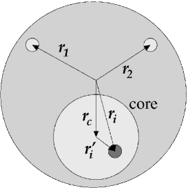
Figure 9: Coordinates used to calculate the ${\cal M}_{\mu}(E\lambda)$ operator in ¹²Be three-body cluster. $\bm{r}_{1}$, $\bm{r}_{2}$ and $\bm{r}_{c}$ give the positions of the three components relative to the center-of-mass of the system. The coordinate of the particle $i$ inside the core is written as $\bm{r}_{i}=\bm{r}_{c}+\bm{r^{\prime}_{i}}$ where $\bm{r^{\prime}_{i}}$ is its position relative to the core center-of-mass.

For the particular case of ¹²Be, we are assuming that the system is clustered, showing a three-body structure made by a core (containing $A-2$ nucleons) plus two additional nucleons outside the core. It is then convenient to write the coordinates of the particles inside the core as: $\bm{r}_{i}=\bm{r}_{c}+\bm{r^{\prime}_{i}}$, where $\bm{r}_{c}$ gives the position of the core center of mass relative to the $A$-body center-of-mass, and $\bm{r^{\prime}_{i}}$ is the coordinate of constituent $i$ in the core relative to the core center-of-mass (see Fig.9).

The ${\cal M}_{\mu}(E\lambda)$ operator in Eq.(19) can then be rewritten as:

$${\cal M}_{\mu}(E\lambda) = e\sum_{i=1}^{A-2}Z_{i}|\bm{r}_{c}+\bm{r}_{i}^{\prime}|^{\lambda}Y_{\lambda,\mu}(\widehat{\bm{r}_{c}+\bm{r}_{i}^{\prime}})$$ (20)

$$+ e\sum_{j=1}^{2}Z_{j}r_{j}^{\lambda}Y_{\lambda,\mu}(\hat{r}_{j})$$

where the index $i$ runs over the $A-2$ constituents in the core, and $j$ labels the two external nucleons.

Making use of Eq.(1) in ref.dix73 (see also dix74 ) one can easily see that for $\lambda=1$ one has:

$${\cal M}_{\mu}(E1)=e\sum_{i=1}^{3}Z_{i}r_{i}Y_{1,\mu}(\hat{r}_{i})+{\cal M}_{\mu}(E1,core)$$ (21)

where now $i$ runs over the three constituents, $Z_{i}$ refers to the charge (in units of $e$) of each of the three constituents, and ${\cal M}_{\mu}(E1,core)=e\sum_{i=1}^{A-2}Z_{i}r^{\prime}_{i}Y_{1,\mu}(\hat{r}_{i}^{\prime})$ is the electric dipole transition operator of the core.

In the same way, for $\lambda=2$ one finds:

$${\cal M}_{\mu}(E2) = e\sum_{i=1}^{3}Z_{i}r^{2}_{i}Y_{2,\mu}(\hat{r}_{i})+{\cal M}_{\mu}(E2,core)$$

$$+ \sum_{m=-1}^{1}f(m,\mu)r_{c}Y_{1,m}(\hat{r}_{c}){\cal M}_{\mu-m}(E1,core)$$

whose two first terms are analogous to the ones in Eq.(21). The last term represents a coupling between the intrinsic core dipole operator and the dipole operator associated to the center-of-mass of the core while $f(m,\mu)$ is a well defined function of the indices $m$ and $\mu$.

References

- (1) F. Ajzenberg-Selove, Nucl. Phys. A 248,1 (1975).
- (2) F.C. Barker and G.T. Hickey, J. Phys. G 3, L23 (1977).
- (3) L. Johannsen, A.S. Jensen and P.G. Hansen, Phys. Lett. B 244, 357 (1990).
- (4) I.J. Thompson and M.V. Zhukov, Phys. Rev. C 49, 1904 (1994).
- (5) R.A. Kryger et al., Phys. Rev. C 47, R2439 (1993).
- (6) B.M. Young et al., Phys. Rev. C 49, 279 (1994).
- (7) S.N. Abramovich, B. Ya Guzhovskii and L.M. Lazarev, Phys. Part. Nucl. 26, 423 (1995).
- (8) M. Zinser et al., Phys. Rev. Lett. 75, 1719 (1995).
- (9) H.B. Jeppesen et al., Phys. Lett. B 642, 449 (2006).
- (10) F.C. Barker, J. Phys. G 2, L45 (1976).
- (11) H.T. Fortune, G.-B. Liu, and D.E. Alburger, Phys. Rev. C 50, 1355 (1994).
- (12) A. Navin et al., Phys. Rev. Lett. 85, 266 (2000).
- (13) S.D. Pain et al., Phys. Rev. Lett. 96, 032502 (2006).
- (14) E. Garrido, D.V. Fedorov, and A.S. Jensen, Nucl. Phys. A700, 117 (2002).
- (15) M. Zinser et al., Nucl. Phys. A619, 151 (1997).
- (16) M.V. Zhukov, B.V. Danilin, D.V. Fedorov, J.M. Bang, I.J. Thompson and J.S. Vaagen, Phys. Rep. 231, 151 (1993).
- (17) E. Garrido, D.V. Fedorov and A.S. Jensen, Nucl. Phys. A 695, 109 (2001).
- (18) M. Fukuda et al., Phys. Lett. B 268, 339 (1991).
- (19) R. Anne et al., Phys. Lett. B 304, 55 (1993).
- (20) J.H. Kelley et al., Phys. Rev. Lett. 74, 30 (1995).
- (21) W.D. Teeters and D. Kurath, Nucl. Phys. A 275, 61 (1977).
- (22) T. Otsuka, N. Fukunishi and H. Sagawa, Phys. Rev. Lett. 70, 1385 (1993).
- (23) H. Esbensen, B.A. Brown and H. Sagawa, Phys. Rev. C 51, 1274 (1995).
- (24) P. Descouvemont, Nucl. Phys. A 615, 261 (1997).
- (25) N. Vinh-Mau, Nucl. Phys. A 592, 33 (1995).
- (26) F.M. Nunes, I.J. Thompson and R.C. Johnson, Nucl. Phys. A 596, 171 (1996).
- (27) S. Fortier et al., Phys. Lett. B 461, 22 (1999).
- (28) J.S. Winfield et al., Nucl. Phys. A 683, 48 (2001).
- (29) F.M. Nunes, J.A. Christley, I.J. Thompson, R.C. Johnson and V.D. Efros, Nucl. Phys. A 609, 43 (1996).
- (30) D.E. Alburger et al., Phys. Rev. C 17, 1525 (1978).
- (31) H. Iwasaki et al., Phys. Lett. B 481, 7 (2000).
- (32) H. Iwasaki et al., Phys. Lett. B 491, 8 (2000).
- (33) S. Shimoura et al., abstract PH-29, in: ENAM 2001 Conf., Hämeenlinna, Finland, 2-7 July 2001.
- (34) S. Shimoura et al., Phys. Lett. B 560, 31 (2003).
- (35) F.M. Nunes, I.J. Thompson and J.A. Tostevin, Nucl. Phys. A 703, 593 (2002).
- (36) E. Garrido, D.V. Fedorov, and A.S. Jensen, Nucl. Phys. A 617, 153 (1997).
- (37) E. Garrido, D.V. Fedorov, and A.S. Jensen, Phys. Rev. C 59, 1272 (1999).
- (38) B.V. Danilin, I.J. Thompson, J.S. Vaagen, and M.V. Zhukov, Nucl. Phys. A 632, 383 (1998).
- (39) E. Nielsen, D.V. Fedorov, A.S. Jensen and E. Garrido, Phys. Rep. 347, 373 (2001).
- (40) S. Shimoura et al., Phys. Lett. B 654, 87 (2007).
- (41) E. Garrido, D.V. Fedorov, and A.S. Jensen, Phys. Rev. C69, 024002 (2004).
- (42) R.B. Wiringa, V.G.J. Stoks and R. Schiavilla, Phys. Rev. C 51, 38 (1995).
- (43) F. Ajzenberg-Selove, Nucl. Phys. A 506, 1 (1990).
- (44) G.-B. Liu and H.T. Fortune, Phys. Rev. C42, 167 (1990).
- (45) D.J. Millener, Nucl. Phys. A 693, 394 (2001).
- (46) N. Fukuda et al., Phys. Rev. C 70, 054606 (2004).
- (47) F. Ajzenberg-Selove, Nucl. Phys. A 490, 1 (1988).
- (48) I. Tanihata, T. Kobayashi, O. Yamakawa, K. Sugimoto, N. Takahashi, T. Shimoda, and H. Sato, Phys. Lett. B 206, 592 (1988).
- (49) E. Garrido, D.V. Fedorov, and A.S. Jensen, Nucl. Phys. A 650, 247 (1999).
- (50) D.J. Morrissey et al., Nucl. Phys. A 627, 222 (1997).
- (51) H.O.U. Fynbo et al., Nucl. Phys. A 736, 39 (2004).
- (52) Y. Hirayama, T. Shimoda, H. Izumi, A. Hatakeyama, K.P. Jackson, C.D.P. Levy, H. Miyatake, M. Yagi and H. Yano, Phys. Lett. B 611, 239 (2005).
- (53) C. Romero-Redondo, E. Garrido, D.V. Fedorov, and A.S. Jensen, Phys. Lett. B 660, 32 (2008).
- (54) D.J. Millener, J.W. Olness, E.K. Warburton, and S.S. Hanna, Phys. Rev. C 28, 497 (1983).
- (55) Y. Suzuki, H. Matsumura, and B. Abu-Ibrahim, Phys. Rev. C 70, 051302(R) (2004).
- (56) W. Horiuchi and Y. Suzuki, Phys. Rev. C 73, 037304 (2006).
- (57) S. Raman, C.H. Malarkey, W.T. Milner, C.W. Nestor Jr., and P.H. Stelson, At. Data and Nucl. Data Tables 36, 1 (1987).
- (58) Y. Kanada-En’yo and H. Horiuchi, Phys. Rev. C 68, 014319 (2003).
- (59) A. Bohr and B.R.Mottelson, Nuclear structure, vol 1 and 2 (Benjamin, Reading Massachusetts, 1969, 1975).
- (60) E. Garrido, D.V. Fedorov, and A.S. Jensen, Phys. Rev. C55, 1327 (1997).
- (61) M. Zahar et al., Phys. Rev. C 48, R1484 (1993).
- (62) J.M. Dixon and R. Lacroix, J. Phys. A 6, 1119 (1973).
- (63) J.M. Dixon and R. Lacroix, J. Phys. A 7, 552 (1974).