Preservation of Positivity by Dynamical Coarse-Graining

Abstract

We compare different quantum Master equations for the time evolution of the reduced density matrix. The widely applied secular approximation (rotating wave approximation) applied in combination with the Born-Markov approximation generates a Lindblad type master equation ensuring for completely positive and stable evolution and is typically well applicable for optical baths. For phonon baths however, the secular approximation is expected to be invalid. The usual Markovian master equation does not generally preserve positivity of the density matrix. As a solution we propose a coarse-graining approach with a dynamically adapted coarse graining time scale. For some simple examples we demonstrate that this preserves the accuracy of the integro-differential Born equation. For large times we analytically show that the secular approximation master equation is recovered. The method can in principle be extended to systems with a dynamically changing system Hamiltonian, which is of special interest for adiabatic quantum computation. We give some numerical examples for the spin-boson model of cases where a spin system thermalizes rapidly, and other examples where thermalization is not reached.

I Introduction

The discovery that quantum computers would have much stronger capabilities for solving certain kinds of problems (such as number factoring shor1997a or database search grover1997a ) than their classical counterparts has initiated a lot of research in quantum information theory nielsen2000 .

Unfortunately, the fragile quantum coherence necessary for the superior performance of quantum computers is very sensitive to the inevitable interaction with the environment such that theoretical understanding of this process – called decoherence – is absolutely necessary breuer2002 .

For simple models (such as, e.g., a single spin or harmonic oscillator coupled to a thermalized bath of harmonic oscillators) and for sufficiently complex couplings to the reservoir after some time the system will equilibrate in a thermal state with the bath temperature breuer2002 . This behavior would be consistent with our classical expectations.

A recent idea is to protect the quantum information by encoding the solution to a given problem in the (unknown) ground state of a problem Hamiltonian $H_{\rm P}$. Given sufficient experimental control of the system Hamiltonian and a reservoir at sufficiently low temperature $k_{\rm B}T\ll\Delta E_{\rm min}$ (where $\Delta E_{\rm min}$ denotes the energy gap above the ground state energy of $H_{\rm P}$), the ground state should be robust against decoherence in the sense that decoherence would always drive the system towards its ground state. In principle, one could then prepare the quantum system in any accessible state and wait sufficiently long until the equilibration has taken place. Unfortunately, this mere-cooling approach is not expected to be very efficient, since the relaxation rate may be very small khidekel1995a or (in extreme cases) the system might get stuck in a local minimum childs2001 .

A possible solution was proposed with the concept of adiabatic quantum computation farhi2001a : The system is initially subject to a simple Hamiltonian $H_{\rm I}$ and is prepared in its (easily accessible) ground state. Then, the Hamiltonian is slowly deformed into the problem Hamiltonian $H_{\rm P}$. The adiabatic theorem states that if this transformation proceeds slowly enough, the quantum state will closely follow the instantaneous ground state sarandy2004a . Finally, for a nearly adiabatic evolution the system state approximates the system ground state to a high degree. Consequently, the maximum transformation rate (where the final excitations are acceptably small) corresponds to the computational complexity of the adiabatic algorithm. For closed systems, it is related to the spectral properties of the time-dependent system Hamiltonian jansen2007a ; schaller2006b . For a reservoir at sufficiently low temperatures, this scheme is thought to be robust against decoherence childs2001 and might even be aided by it amin2008a .

Unfortunately, the standard framework of deriving master equations relies on some prerequisites that are not always fulfilled in realistic systems. For example, the Markovian approximation widely used is usually only formulated for time-independent system Hamiltonians. In addition, it sometimes leads to master equations that do not preserve positivity of the system density matrix zhao2002a ; stenholm2004a . Together with trace preservation, positivity grants stability of the density matrix eigenvalues and is thus necessary for probability interpretation (cf. pechukas1994a ) of the density matrix. Consequently, observables obtained from non-positive density matrices may become unphysical yu2000a . This problem can be cured by the secular approximation. Combined with the Markovian approximation, it leads to Lindblad-type lindblad1976a master equations that generically preserve positivity of the density matrix. Unfortunately, the secular approximation is rather valid for quantum-optical but not for phonon baths breuer2002 . Note that there exist non-Markovian master equations that are not of Lindblad type but nevertheless preserve positivity by construction. These models however are either phenomenologic munro1996a ; wilkie2000a in the sense that their parameters are not derived from a microscopic Hamiltonian or they only grant positivity on a restricted set of initial states tameshtit1996a . Especially in view of an experimental optimization of decoherence effects it is, however, necessary to relate the parameters in the master equation to those in the microscopic Hamiltonian spreeuw2007a . For example, for a realistic implementation of an adiabatic (or gate-model) quantum computer one would expect the qubits to be coupled to phonon degrees of freedom as well, such that a general treatment is advised. The present article shall present a further step in that direction.

It has been noted karrlein1997a ; vacchini2000a ; lidar2001a that coarse-graining may ensure for positive evolution of the reduced density matrix. However, the coarse-graining timescale so far had to be much larger than the inverse of the bath density of states cutoff. In this paper we argue that by adaptively changing the coarse-graining timescale one does not have to obey this constraint. Beyond this, we show that for infinitely large coarse-graining times we reproduce the widely used secular approximation. We show analytically that for any fixed coarse-graining timescale $\tau\geq 0$, the resulting master equations are of Lindblad form, i.e. they preserve positivity and thereby also stability of the density matrix.

This paper is organized as follows: In section II we introduce our notation and in section III we compare the standard procedure of deriving quantum master equations from microscopic models with the proposed adaptive coarse-graining scheme. We make our method explicit by the example of the spin-boson model in section IV.

II General Prerequisites

We will consider Hamiltonians which can be divided into three parts

$$H(t)=H_{\rm S}(t)+H_{\rm SB}+H_{\rm B}\,,$$ (1)

where $H_{\rm S}(t)$ describes the system part, $H_{\rm B}$ the part acting on the bath (with $\left[H_{\rm S}(t),H_{\rm B}\right]=0$) and

$$H_{\rm SB}=\lambda\sum_{\cal A}A_{\cal A}\otimes B_{\cal A}$$ (2)

denotes the interaction Hamiltonian with the small dimensionless coupling parameter $\lambda\ll 1$ and system operators $A_{\cal A}$ as well as bath operators $B_{\cal A}$ (differing coupling constants can be absorbed in the operator definitions). Hermiticity is only required for the complete sum ($H_{\rm SB}=H_{\rm SB}^{\dagger}$), but by splitting operators into hermitian and anti-hermitian parts one can always redefine them such that

$$A_{\cal A}=A_{\cal A}^{\dagger}\,,\qquad B_{\cal A}=B_{\cal A}^{\dagger}\,,$$ (3)

which will be assumed further-on.

The density matrix of the complete system is thought to evolve according to ($\hbar=1$ throughout) the von-Neumann equation of motion

$$\dot{\rho}(t)=-i\left[H_{\rm S}(t)+H_{\rm SB}+H_{\rm B},\rho(t)\right]\,.$$ (4)

Denoting the time evolution operators of system and reservoir by $U(t)$ and $V(t)$, respectively, we can switch to the interaction picture

$$\mbox{\boldmath$\rho$}(t) = U^{\dagger}(t)V^{\dagger}(t)\rho(t)V(t)U(t)\,,$$

$$\mbox{\boldmath$H_{\rm SB}$}(t) = U^{\dagger}(t)V^{\dagger}(t)H_{\rm SB}V(t)U(t)$$ (5)

$$= \lambda\sum_{\cal A}\left[U^{\dagger}(t)A_{\cal A}U(t)\right]\otimes\left[V^{\dagger}(t)B_{\cal A}V(t)\right]$$

$$\equiv \lambda\sum_{\cal A}\mbox{\boldmath$A_{\cal A}$}(t)\otimes\mbox{\boldmath$B_{\cal A}$}(t)\,.$$

We will denote all operators in the interaction picture by bold symbols throughout. In the interaction picture, the equation of motion for the density operator (4) transforms into

$$\mbox{\boldmath$\dot{\rho}$}(t)=-i\left[\mbox{\boldmath$H_{\rm SB}$}(t),\mbox{\boldmath$\rho$}(t)\right]\,,$$ (6)

where one can exploit the smallness of the coupling $\lambda$ to apply perturbation theory.

Equation (6) can be formally integrated to yield $\mbox{\boldmath$\rho$}(t)=\mbox{\boldmath$\rho$}(0)-i\int\limits_{0}^{t}\left[\mbox{\boldmath$H_{\rm SB}$}(t^{\prime}),\mbox{\boldmath$\rho$}(t^{\prime})\right]dt^{\prime}$ and re-inserting this result in Eqn. (6) one obtains the following exact equation

$$\dot{\mbox{\boldmath$\rho$}}(t) = -i\left[\mbox{\boldmath$H_{\rm SB}$}(t),\mbox{\boldmath$\rho$}(0)\right]$$ (7)

$$-\int\limits_{0}^{t}\left[\mbox{\boldmath$H_{\rm SB}$}(t),\left[\mbox{\boldmath$H_{\rm SB}$}(t^{\prime}),\mbox{\boldmath$\rho$}(t^{\prime})\right]\right]dt^{\prime}$$

for the density operator.

III Quantum Master Equations

We will first state the results of the Born-Markov approximation without secular approximation (in subsection III.1) and with the secular approximation (subsection III.2) in our notation. Afterwards, we will consider the coarse-graining approach in subsection III.3.

With the usual assumptions (compare Appendix A) involving initial factorization of the density matrix and neglecting any change in the reservoir part of the density matrix in (7) we obtain the Born equation

$$\dot{\rho_{\rm S}} = -i{\rm Tr_{B}}\left\{\left[\mbox{\boldmath$H_{\rm SB}$}(t),\mbox{\boldmath$\rho_{\rm S}$}(0)\mbox{\boldmath$\rho_{\rm B}^{0}$}\right]\right\}$$ (8)

$$-\int\limits_{0}^{t}{\rm Tr_{B}}\left\{\left[\mbox{\boldmath$H_{\rm SB}$}(t),\left[\mbox{\boldmath$H_{\rm SB}$}(t^{\prime}),\mbox{\boldmath$\rho_{\rm S}$}(t^{\prime})\mbox{\boldmath$\rho_{\rm B}^{0}$}\right]\right]\right\}dt^{\prime}$$

$$+{\cal O}\{\lambda^{3}\}\,,$$

where ${\rm Tr_{B}}\left\{\cdot\right\}$ denotes the trace over the reservoir degrees of freedom. Evaluating the traces leads to the definition of the reservoir correlation functions

$$C_{\cal AB}(\tau) \equiv {\rm Tr_{B}}\left\{e^{+iH_{\rm B}\tau}B_{\cal A}e^{-iH_{\rm B}\tau}B_{\cal B}\rho_{\rm B}^{0}\right\}$$ (9)

$$= C_{\cal BA}^{*}(-\tau)\,,$$

and we obtain with $\left<B_{\cal A}\right>=0$ (which can always be achieved by a suitable transformation trafo )

$$\dot{\mbox{\boldmath$\rho_{\rm S}$}} = \lambda^{2}\sum_{\cal AB}\int\limits_{0}^{t}\Big{\{}\left[\mbox{\boldmath$A_{\cal B}$}(t^{\prime})\mbox{\boldmath$\rho_{\rm S}$}(t^{\prime}),\mbox{\boldmath$A_{\cal A}$}(t)\right]C_{\cal AB}(t-t^{\prime})$$ (10)

$$+{\rm h.c.}\Big{\}}\,dt^{\prime}+{\cal O}\{\lambda^{3}\}\,,$$

where h.c. denotes the hermitian conjugate. The integro-differential character of above equation complicates its solution, since analytical solutions are only possible in very simple cases kleinekathoefer2004a ; schroeder2007a (see also subsection IV.2), and numerical solutions are hampered by the fact that the complete history of $\mbox{\boldmath$\rho_{\rm S}$}(t^{\prime})$ has to be stored in order to evolve $\mbox{\boldmath$\rho_{\rm S}$}(t)$.

III.1 Markovian approximation scheme

In the usual breuer2002 Markovian approximation (see Appendix B) one obtains for constant system Hamiltonians ($H_{\rm S}(t)=H_{\rm S}$) with the half-sided Fourier transforms

$$\Gamma_{\cal AB}(\omega) \equiv \int\limits_{0}^{\infty}C_{\cal AB}(\tau)e^{i\omega\tau}d\tau$$ (11)

of the reservoir correlation functions (9) the time-local Born-Markov (BM) master equation (here given in the Schrödinger picture)

$$\dot{\rho_{\rm S}} = -i\left[H_{\rm S},\rho_{\rm S}(t)\right]$$ (12)

$$+\lambda^{2}\sum_{abcd}\sum_{\cal AB}\Big{\{}\Gamma_{\cal AB}(E_{b}-E_{a})\times$$

$$\times\left<a\right|A_{\cal B}\left|b\right>\left<c\right|A_{\cal A}\left|d\right>^{*}\left[\Big{(}\left|a\right>\left<b\right|\Big{)}\rho_{\rm S}(t),\Big{(}\left|c\right>\left<d\right|\Big{)}^{\dagger}\right]$$

$$+{\rm h.c.}\Big{\}}\,,$$

where $H_{\rm S}\left|a\right>=E_{a}\left|a\right>$ denote the orthonormal energy eigenbasis. By construction, Eqn. (12) does preserve trace and hermiticity of $\rho_{\rm S}$. Note however, that positivity of its solution $\rho_{\rm S}(t)$ is not generally preserved zhao2002a ; whitney2008a , see subsection IV.4 for some counterexamples.

III.2 The secular approximation

In order to restore preservation of positivity in the BM approximation in general, it is necessary to perform the secular approximation (see Appendix C). Typically, this approximation is known to be well-satisfied for quantum-optical systems, where it is also known as rotating wave approximation scully2002 . In this case, one can combine

$$\gamma_{\cal AB}(\omega) = \Gamma_{\cal AB}(\omega)+\Gamma_{\cal BA}^{*}(\omega)=\int\limits_{-\infty}^{+\infty}C_{\cal AB}(\tau)e^{i\omega\tau}d\tau\,,$$

$$\sigma_{\cal AB}(\omega) = \Gamma_{\cal AB}(\omega)-\Gamma_{\cal BA}^{*}(\omega)$$ (13)

$$= \int\limits_{-\infty}^{+\infty}C_{\cal AB}(\tau){\rm sgn}(\tau)e^{i\omega\tau}d\tau$$

which yields the Born-Markov-Secular (BMS) approximation (in the Schrödinger picture)

$$\dot{\rho_{\rm S}} = -i\left[H_{\rm S},\rho_{\rm S}(t)\right]$$

$$-i\left[\sum_{ab}\tilde{\sigma}_{ab}\left|a\right>\left<b\right|,\rho_{\rm S}(t)\right]$$

$$+\sum_{abcd}\tilde{\gamma}_{ab,cd}\Big{[}\Big{(}\left|a\right>\left<b\right|\Big{)}\rho_{\rm S}(t)\Big{(}\left|c\right>\left<d\right|\Big{)}^{\dagger}$$

$$-\frac{1}{2}\left\{\Big{(}\left|c\right>\left<d\right|\Big{)}^{\dagger}\Big{(}\left|a\right>\left<b\right|\Big{)},\rho_{\rm S}(t)\right\}\Big{]}\,,$$

$$\tilde{\sigma}_{ab} = \frac{\lambda^{2}}{2i}\sum_{c}\sum_{\cal AB}\sigma_{\cal AB}(E_{a}-E_{c})\delta_{E_{b},E_{a}}\times$$

$$\times\left<c\right|A_{\cal A}\left|a\right>^{*}\left<c\right|A_{\cal B}\left|b\right>\,,$$

$$\tilde{\gamma}_{ab,cd} = \lambda^{2}\sum_{\cal AB}\gamma_{\cal AB}(E_{b}-E_{a})\delta_{E_{d}-E_{c},E_{b}-E_{a}}\times$$ (14)

$$\times\left<a\right|A_{\cal B}\left|b\right>\left<c\right|A_{\cal A}\left|d\right>^{*}\,.$$

Eqn. (III.2) has many favorable properties (compare e.g. chapter 3.3 in breuer2002 ):

By construction, it preserves trace and hermiticity of the system density matrix $\rho_{\rm S}$.

Since it is of Lindblad lindblad1976a form (the matrix $\gamma_{\cal AB}(\omega)$ is positive semidefinite), it preserves positivity of the density matrix.

For a thermalized reservoir characterized by the inverse temperature $\beta$, the Fourier transforms of the bath correlation functions can be used to show that the system thermal equilibrium state with the same temperature

$$\rho_{\rm S}^{\rm th}=\frac{e^{-\beta H_{\rm S}}}{{\rm Tr_{S}}\left\{e^{-\beta H_{\rm S}}\right\}}$$ (15)

is a stationary state.

If the spectrum of the system Hamiltonian $H_{\rm S}$ is non-degenerate (implying that $\delta_{E_{a},E_{b}}=\delta_{ab}$), the equations for the diagonal elements of $\rho_{\rm S}$ in the eigenbasis of $H_{\rm S}$ completely decouple from the equations for the off-diagonals, and one obtains the same transition rates between the populations as with Fermis Golden Rule.

III.3 Coarse-graining approach

Eqn. (6) is formally solved by $\mbox{\boldmath$\rho$}(t_{2})=\mbox{\boldmath$W$}(t_{2},t_{1})\mbox{\boldmath$\rho$}(t_{1})\mbox{\boldmath$W$}^{\dagger}(t_{2},t_{1})$ with the interaction picture time evolution operator

$$\mbox{\boldmath$W$}(t_{2},t_{1})={\cal T}\exp\left\{-i\int\limits_{t_{1}}^{t_{2}}\mbox{\boldmath$H_{\rm SB}$}(t^{\prime})dt^{\prime}\right\}\,,$$ (16)

where the time-dependence of $\mbox{\boldmath$H_{\rm SB}$}(t)$ necessitates the time-ordering scully2002 ${\cal T}\mbox{\boldmath$H_{\rm SB}$}(t_{1})\mbox{\boldmath$H_{\rm SB}$}(t_{2})\equiv\mbox{\boldmath$H_{\rm SB}$}(t_{1})\mbox{\boldmath$H_{\rm SB}$}(t_{2})\Theta(t_{1}-t_{2})+\mbox{\boldmath$H_{\rm SB}$}(t_{2})\mbox{\boldmath$H_{\rm SB}$}(t_{1})\Theta(t_{2}-t_{1})$, with $\Theta(x)$ denoting the Heavyside step function. Now, by expanding $\mbox{\boldmath$W$}(t+\tau,t)$ up to second order in $\lambda$ we obtain a second-order approximation to the full density matrix

$$\mbox{\boldmath$\rho$}(t+\tau) = \mbox{\boldmath$\rho$}(t)-i\left[\int\limits_{t}^{t+\tau}\mbox{\boldmath$H_{\rm SB}$}(t_{1})dt_{1},\mbox{\boldmath$\rho$}(t)\right]-i\left[\frac{1}{2i}\int\limits_{t}^{t+\tau}\int\limits_{t}^{t+\tau}\left[\mbox{\boldmath$H_{\rm SB}$}(t_{2}),\mbox{\boldmath$H_{\rm SB}$}(t_{1})\right]\Theta(t_{2}-t_{1})dt_{1}dt_{2},\mbox{\boldmath$\rho$}(t)\right]$$ (17)

$$+\int\limits_{t}^{t+\tau}\int\limits_{t}^{t+\tau}\left[\mbox{\boldmath$H_{\rm SB}$}(t_{1})\mbox{\boldmath$\rho$}(t)\mbox{\boldmath$H_{\rm SB}$}(t_{2})-\frac{1}{2}\left\{\mbox{\boldmath$H_{\rm SB}$}(t_{2})\mbox{\boldmath$H_{\rm SB}$}(t_{1}),\mbox{\boldmath$\rho$}(t)\right\}\right]dt_{1}dt_{2}+{\cal O}\left\{\lambda^{3}\right\}\,.$$

Since such a truncated finite order approximation to the time evolution operator $\mbox{\boldmath$W$}(t+\tau)$ is still unitary, the above map (17) preserves hermiticity, trace and positivity of the full density matrix $\rho$. An equivalent expression can be obtained from iterative solution of equation (7) by keeping only terms up to ${\cal O}\{\lambda^{2}\}$. We will proceed with this second order approximation and derive from this fully unitary map a non-unitary map for the system part of the density matrix that preserves positivity.

If we neglect the back-action of the system on the bath and assume factorization (Born-approximation) as described in Appendix A we can perform the partial trace over the reservoir degrees of freedom. By inserting the definition (2) in Eqn. (17) and employing the definition of the reservoir correlation functions (9) we obtain (again working in a frame where $\left<B_{\cal A}\right>=0$ trafo )

$$\mbox{\boldmath$\rho_{\rm S}$}(t+\tau) = \mbox{\boldmath$\rho_{\rm S}$}(t)$$ (18)

$$-i\frac{\lambda^{2}}{2i}\sum_{\cal AB}\int\limits_{t}^{t+\tau}\int\limits_{t}^{t+\tau}C_{\cal AB}(t_{2}-t_{1}){\rm sgn}(t_{2}-t_{1})\times$$

$$\times\left[\mbox{\boldmath$A_{\cal A}$}(t_{2})\mbox{\boldmath$A_{\cal B}$}(t_{1}),\mbox{\boldmath$\rho_{\rm S}$}(t)\right]dt_{1}dt_{2}$$

$$+\lambda^{2}\sum_{\cal AB}\int\limits_{t}^{t+\tau}\int\limits_{t}^{t+\tau}C_{\cal AB}(t_{2}-t_{1})\times$$

$$\times\Big{[}\mbox{\boldmath$A_{\cal B}$}(t_{1})\mbox{\boldmath$\rho_{\rm S}$}(t)\mbox{\boldmath$A_{\cal A}$}(t_{2})$$

$$-\frac{1}{2}\left\{\mbox{\boldmath$A_{\cal A}$}(t_{2})\mbox{\boldmath$A_{\cal B}$}(t_{1}),\mbox{\boldmath$\rho_{\rm S}$}(t)\right\}\Big{]}dt_{1}dt_{2}+{\cal O}\{\lambda^{3}\}$$

$$\equiv \mbox{\boldmath$\rho_{\rm S}$}(t)+\tau\mbox{\boldmath$L^{\tau}$}(t)\mbox{\boldmath$\rho_{\rm S}$}(t)+{\cal O}\{\lambda^{3}\}\,,$$

which defines the action of the Liouvillian on the reduced density matrix in the interaction picture. If one re-arranges the matrix elements of the density matrix as a $N^{2}$-dimensional vector, the Liouvillian super-operator can be understood as an $N^{2}\times N^{2}$ (generally non-hermitian) matrix acting on $\rho_{\rm S}$. In the interaction picture the Liouvillian is small, i.e., since $\left<B_{\cal A}\right>=0$ we even have $\mbox{\boldmath$L^{\tau}$}={\cal O}\{\lambda^{2}\}$.

Unfortunately, the above map $\mbox{\boldmath$\rho_{\rm S}$}(t)\to\mbox{\boldmath$\rho_{\rm S}$}(t+\tau)$ has some shortcomings: It does not generally preserve positivity of the reduced density matrix $\rho_{\rm S}$ and in addition, if one applies above equation recursively $n$-times with small timesteps $\Delta\tau$ such that $n\Delta\tau=\tau$ and compares the result with a single iteration of (18), the difference between the two solutions is much larger than ${\cal O}\{\lambda^{3}\}$, i.e., the solution depends on the choice of the stepsize.

By defining time-averaging of an operator ${\cal\hat{O}}(t)$ over a time interval $[t,t+\tau]$ as

$${\left<\left<\cal\hat{O}\right>\right>}_{[t,t+\tau]}\equiv\frac{1}{\tau}\int\limits_{t}^{t+\tau}{\cal\hat{O}}(t^{\prime})dt^{\prime}\,,$$ (19)

we can write Eqn. (18) as

$${\left<\left<\mbox{\boldmath$\dot{\rho}_{\rm S}$}\right>\right>}_{[t,t+\tau]} = \frac{\mbox{\boldmath$\rho_{\rm S}$}(t+\tau)-\mbox{\boldmath$\rho_{\rm S}$}(t)}{\tau}$$ (20)

$$= \mbox{\boldmath$L^{\tau}$}(t)\mbox{\boldmath$\rho_{\rm S}$}(t)+{\cal O}\{\lambda^{3}\}\,.$$

III.3.1 Explicit Liouvillian

It is convenient to insert the even and odd Fourier transforms from (III.2) of the reservoir correlation functions

$$C_{\cal AB}(\tau) = \frac{1}{2\pi}\int\limits_{-\infty}^{+\infty}\gamma_{\cal AB}(\omega)e^{-i\omega\tau}d\omega\,,$$

$$C_{\cal AB}(\tau){\rm sgn}(\tau) = \frac{1}{2\pi}\int\limits_{-\infty}^{+\infty}\sigma_{\cal AB}(\omega)e^{-i\omega\tau}d\omega\,,$$ (21)

and to expand the system operators in the interaction picture in the orthonormal energy eigenbasis $H_{\rm S}\left|a\right>=E_{a}\left|a\right>$ of the system Hamiltonian (here assumed to be constant)

$$\mbox{\boldmath$A_{\cal A}$}(t_{2}) = \sum_{ab}\left<a\right|A_{\cal A}\left|b\right>e^{i(E_{a}-E_{b})t_{2}}\left|a\right>\left<b\right|\,,$$

$$\mbox{\boldmath$A_{\cal B}$}(t_{1}) = \sum_{cd}\left<c\right|A_{\cal B}\left|d\right>e^{i(E_{c}-E_{d})t_{1}}\left|c\right>\left<d\right|\,.$$ (22)

Then, we can use the relation $\int\limits_{t}^{t+\tau}e^{i\alpha t^{\prime}}dt^{\prime}=\tau e^{i\alpha t}e^{i\alpha\tau/2}{\rm sinc}\left[\frac{\alpha\tau}{2}\right]$ with ${\rm sinc}\left[x\right]\equiv\frac{\sin(x)}{x}$ together with Eqn. (III.3.1) and Eqn. (III.3.1) in order to make the Liouvillian in Eqn. (20) explicit. With denoting the energy differences of the system Hamiltonian by $\Omega_{ab}\equiv E_{a}-E_{b}$ we arrive at

$$\mbox{\boldmath$L^{\tau}$}(t)\mbox{\boldmath$\rho_{\rm S}$}(t) = -i\left[\sum_{ab}e^{i\Omega_{ab}t}\sigma_{ab}(\tau)\left|a\right>\left<b\right|,\mbox{\boldmath$\rho_{\rm S}$}(t)\right]$$

$$+\sum_{abcd}e^{i(\Omega_{cd}-\Omega_{ab})t}\gamma_{cd,ba}(\tau)\left[\Big{(}\left|c\right>\left<d\right|\Big{)}\mbox{\boldmath$\rho_{\rm S}$}(t)\Big{(}\left|b\right>\left<a\right|\Big{)}^{\dagger}-\frac{1}{2}\left\{\Big{(}\left|b\right>\left<a\right|\Big{)}^{\dagger}\Big{(}\left|c\right>\left<d\right|\Big{)},\mbox{\boldmath$\rho_{\rm S}$}(t)\right\}\right]\,,$$

$$\sigma_{ab}(\tau) = \frac{\lambda^{2}\tau}{4\pi i}e^{i\Omega_{ab}\tau/2}\sum_{c}\sum_{\cal AB}\left<c\right|A_{\cal A}\left|a\right>^{*}\left<c\right|A_{\cal B}\left|b\right>\int\limits_{-\infty}^{+\infty}\sigma_{\cal AB}(\omega){\rm sinc}\left[(w+\Omega_{ca})\frac{\tau}{2}\right]{\rm sinc}\left[(w+\Omega_{cb})\frac{\tau}{2}\right]d\omega\,,$$

$$\gamma_{cd,ba}(\tau) = \frac{\lambda^{2}\tau}{2\pi}e^{i(\Omega_{cd}-\Omega_{ba})\tau/2}\sum_{\cal AB}\left<b\right|A_{\cal A}\left|a\right>^{*}\left<c\right|A_{\cal B}\left|d\right>\int\limits_{-\infty}^{+\infty}\gamma_{\cal AB}(\omega){\rm sinc}\left[(w+\Omega_{ba})\frac{\tau}{2}\right]{\rm sinc}\left[(w+\Omega_{cd})\frac{\tau}{2}\right]d\omega\,.$$ (23)

The coarse-grained derivative on the l. h. s. of Eqn. (20) generates a time evolution that can be compared with its usual, first order differential equation counterpart (we denote the corresponding density operators by an overbar and the continuous index $\tau$ referring to the Liouvillian chosen)

$$\frac{d}{dt}\mbox{\boldmath$\bar{\rho_{\rm S}^{\tau}}$}(t) = \mbox{\boldmath$L^{\tau}$}(t)\mbox{\boldmath$\bar{\rho_{\rm S}^{\tau}}$}(t)\,.$$ (24)

If we initialize this differential equation with a known density matrix $\rho_{\rm S}^{0}$ and evaluate its formal solution at time $t=\tau$ (i.e., after exactly the coarse-graining timescale), we find to first order in $L^{\tau}$

$$\mbox{\boldmath$\bar{\rho_{\rm S}^{\tau}}$}(\tau) \approx \left[\mbox{\boldmath$1$}+\int\limits_{0}^{\tau}\mbox{\boldmath$L^{\tau}$}(t^{\prime})dt^{\prime}\right]\mbox{\boldmath$\rho_{\rm S}^{0}$}\,.$$ (25)

This means that when considering the same initial condition, the difference between the two time evolutions resulting from Eqns. (24) and (20) is given by

$$\mbox{\boldmath$\bar{\rho_{\rm S}^{\tau}}$}(\tau)-\mbox{\boldmath$\rho_{\rm S}$}(\tau) = \eta(\tau)+{\cal O}\{\left(\mbox{\boldmath$L^{\tau}$}\right)^{2}\}\,,$$

$$\eta(\tau) = \left[\int\limits_{0}^{\tau}\mbox{\boldmath$L^{\tau}$}(t^{\prime})dt^{\prime}-\tau\mbox{\boldmath$L^{\tau}$}(0)\right]\mbox{\boldmath$\rho_{\rm S}^{0}$}\,,$$ (26)

i.e., essentially by the difference between the coarse-graining-averaged Liouvillian and its initial value.

It follows from Eqn. (III.3.1) that especially for short coarse graining times $\tau\ll\frac{1}{{\left|\Delta E_{\rm max}\right|}}$ (with $\Delta E_{\rm max}$ denoting the maximum energy difference of $H_{\rm S}$) the difference will be negligible $\eta(\tau)\approx 0$, such that the two solutions $\mbox{\boldmath$\bar{\rho_{\rm S}^{\tau}}$}(\tau)$ and $\mbox{\boldmath$\rho_{\rm S}$}(\tau)$ are equivalent. Since we have so far not made any assumption on separating timescales, this also implies that non-Markovian effects (that are expected for short times where the Markovian approximation does not hold) are within reach of the adaptive coarse-graining approach, where the coarse-graining time is chosen to match the physical time.

In the limit of very large coarse-graining times we also obtain $\lim\limits_{\tau\to\infty}\eta(\tau)\approx\mbox{\boldmath$0$}$, since then the ${\rm sinc}\left[\cdot\right]$ functions in (III.3.1) begin to act like delta functions, see below.

Also for intermediate coarse-graining times it is easy to see from the structure of the Liouvillian (III.3.1) that the difference $\eta(\tau)$ is bounded throughout.

From now on, we will omit the overbar and write $\rho_{\rm S}^{\tau}(t)$ for the solutions of Eqn. (24).

III.3.2 The infinite-$\tau$ limit

In the limit $\tau\to\infty$ one should note that for discrete $a,b$ and under an integral over $d\omega$ with another integrable function one has in a distributive sense (see Appendix F)

$$f(\omega,a,b) \equiv \lim_{\tau\to\infty}\tau\;{\rm sinc}\left[(w+a)\frac{\tau}{2}\right]{\rm sinc}\left[(w+b)\frac{\tau}{2}\right]$$ (27)

$$\asymp 2\pi\delta_{ab}\delta(w+a)\,,$$

where $\delta_{ab}$ is a Kronecker symbol and $\delta(w+a)$ denotes the Dirac Delta distribution. Therefore, we obtain for the Liouvillian matrix elements (III.3.1) in this limit

$$\sigma_{ab}^{\infty} = \frac{\lambda^{2}}{2i}\delta_{E_{a},E_{b}}\sum_{c}\sum_{\cal AB}\left<c\right|A_{\cal A}\left|a\right>^{*}\left<c\right|A_{\cal B}\left|b\right>\times$$

$$\times\sigma_{\cal AB}(E_{a}-E_{c})\,,$$

$$\gamma_{cd,ba}^{\infty} = \lambda^{2}\delta_{E_{b}-E_{a},E_{c}-E_{d}}\sum_{\cal AB}\left<b\right|A_{\cal A}\left|a\right>^{*}\times$$ (28)

$$\times\left<c\right|A_{\cal B}\left|d\right>\gamma_{\cal AB}(E_{a}-E_{b})\,,$$

and we recover the secular approximation (III.2)! Naturally, this also implies that in the large-time limit, the solution $\mbox{\boldmath$\rho_{\rm S}^{\tau=t}$}(t)$ captures all the favorable properties of Eqn. (III.2).

III.3.3 Positivity

The most striking advantage of the coarse-graining procedure is that not only for very large, but for any fixed coarse-graining time $\tau\geq 0$, the resulting first-order differential equations (24) are all of Lindblad form lindblad1976a and thus intrinsically preserve the positivity of the density matrix. This is easily seen by switching back to the Schrödinger picture, where the time-dependent phases in (III.3.1) cancel

$$\dot{\rho_{\rm S}^{\tau}}(t) \equiv L^{\tau}\rho_{\rm S}^{\tau}(t)$$ (29)

$$= -i\left[H_{\rm S},\rho_{\rm S}^{\tau}(t)\right]$$

$$-i\left[\sum_{ab}\sigma_{ab}(\tau)\left|a\right>\left<b\right|,\rho_{\rm S}^{\tau}(t)\right]$$

$$+\sum_{abcd}\gamma_{cd,ba}(\tau)\Bigg{[}\Big{(}\left|c\right>\left<d\right|\Big{)}\rho_{\rm S}^{\tau}(t)\Big{(}\left|b\right>\left<a\right|\Big{)}^{\dagger}$$

$$-\frac{1}{2}\left\{\Big{(}\left|b\right>\left<a\right|\Big{)}^{\dagger}\Big{(}\left|c\right>\left<d\right|\Big{)},\rho_{\rm S}^{\tau}(t)\right\}\Bigg{]}\,,$$

which implies that the Schrödinger picture Liouvillian $L^{\tau}$ only depends on the coarse-graining timescale $\tau$.

First of all, the first two commutator terms correspond to commutators with a hermitian operator, i.e., the second term accounts for the unitary action of decoherence (sometimes called Lamb-shift breuer2002 ). Note that hermiticity of the corresponding effective Hamiltonian follows from the definition of the odd Fourier transform versus the half-sided Fourier transform (III.2).

In order to show that (29) is a Lindblad form, it remains to be shown that the matrix $\gamma_{cd,ba}(\tau)$ is positive semidefinite. In order to see this we introduce the double indices $i=(cd)$ and $j=(ba)$ running from 1 to $N^{2}$ for an $N$-dimensional system Hilbert space. Then, we can use the short-hand notation $w_{i}=E_{c}-E_{d}$, $A_{\cal B}^{i}=\left<c\right|A_{\cal B}\left|d\right>$, $w_{j}=E_{b}-E_{a}$, $A_{\cal A}^{j}=\left<b\right|A_{\cal A}\left|a\right>$ and consider for arbitrary complex-valued numbers $x_{j}$ in Eqn. (III.3.1)

$$\sum_{ij}x_{i}^{*}\gamma_{ij}x_{j} = \frac{\tau}{2\pi}\int\limits_{-\infty}^{+\infty}\sum_{\cal AB}z_{\cal A}^{*}(\omega)\gamma_{\cal AB}(\omega)z_{\cal B}(\omega)d\omega\,,$$ (30)

where we have

$$z_{\cal A} \equiv \sum_{j}A_{\cal A}^{j}{\rm sinc}\left[(w+w_{j})\tau/2\right]e^{i\omega_{j}\tau/2}x_{j}\,.$$ (31)

Now, since the Fourier-transform matrix $\gamma_{\cal AB}(\omega)$ is positive semidefinite (compare also appendix C) one has $z_{\cal A}^{*}(\omega)\gamma_{\cal AB}(\omega)z_{\cal B}(\omega)\geq 0$. The integral over a strictly positive function can only yield positive results, and since also $\tau\geq 0$ it follows that $\gamma_{ij}(\tau)=\gamma_{cd,ba}(\tau)$ is a positive semidefinite matrix.

This also implies that solutions of the form $\rho_{\rm S}^{t}(t)$ are always positive density matrices, since they correspond to an interpolation along Lindblad density matrices.

III.4 Time-dependent Generalization

Within the coarse-graining approach, it was in Eqn. (III.3.1) where it was used for the first time that the system Hamiltonian $H_{\rm S}$ was time-independent and had a discrete spectrum. Here we will show that coarse-graining generally leads to a time-inhomogeneous (i.e., one with time-dependent operators) Lindblad form of master equations and thus always preserves positivity of the density matrix. With introducing the notation

$$\mbox{\boldmath$\tilde{A}_{\cal A}$}(t,\omega)\equiv\mbox{\boldmath$A_{\cal A}$}(t)e^{i\omega t}$$ (32)

we can use equations (III.3.1) and (19) in Eqn. (18) to obtain

$${\left<\left<\mbox{\boldmath$\dot{\rho}_{\rm S}$}\right>\right>}_{[t,t+\tau]} = -i\left[\frac{\lambda^{2}\tau}{4\pi i}\int\limits_{-\infty}^{+\infty}\sum_{\cal AB}\sigma_{\cal AB}(\omega){\left<\left<\mbox{\boldmath$\tilde{A}_{\cal A}$}(\omega)\right>\right>}_{[t,t+\tau]}^{\dagger}{\left<\left<\mbox{\boldmath$\tilde{A}_{\cal B}$}(\omega)\right>\right>}_{[t,t+\tau]}d\omega,\mbox{\boldmath$\rho_{\rm S}$}(t)\right]$$ (33)

$$+\frac{\lambda^{2}\tau}{2\pi}\int\limits_{-\infty}^{+\infty}\sum_{\cal AB}\gamma_{\cal AB}(\omega)\left[{\left<\left<\mbox{\boldmath$\tilde{A}_{\cal B}$}(\omega)\right>\right>}_{[t,t+\tau]}\mbox{\boldmath$\rho_{\rm S}$}(t){\left<\left<\mbox{\boldmath$\tilde{A}_{\cal A}$}(\omega)\right>\right>}_{[t,t+\tau]}^{\dagger}\right.$$

$$\left.-\frac{1}{2}\left\{{\left<\left<\mbox{\boldmath$\tilde{A}_{\cal A}$}(\omega)\right>\right>}_{[t,t+\tau]}^{\dagger}{\left<\left<\mbox{\boldmath$\tilde{A}_{\cal B}$}(\omega)\right>\right>}_{[t,t+\tau]},\mbox{\boldmath$\rho_{\rm S}$}(t)\right\}\right]\,.$$

With the replacements ${\left<\left<\mbox{\boldmath$\dot{\rho}_{\rm S}$}\right>\right>}_{[t,t+\tau]}\to\mbox{\boldmath$\dot{\rho}_{\rm S}^{\tau}$}$ and $\mbox{\boldmath$\rho_{\rm S}(t)$}\to\mbox{\boldmath$\rho_{\rm S}^{\tau}$}(t)$ this becomes a time-inhomogeneous Lindblad master equation, since the positivity of the $\gamma_{\cal AB}(\omega)$-matrix at every $\omega$ is guaranteed for reservoirs in thermal equilibrium. Intuitively, the time-dependence of the Lindblad operators does not destroy positivity, since at any fixed time $t$ one may approximate the time-dependent operators by a constant-operator Lindblad form, see Appendix E for a more explicit discussion. Since the case of slowly varying system Hamiltonians is of special interest in the context of adiabatic quantum computation childs2001 , we outline in Appendix D how one could in principle calculate the time-averaged operators

$${\left<\left<\mbox{\boldmath$\tilde{A}_{\cal A}$}(\omega)\right>\right>}_{[t,t+\tau]} = \frac{1}{\tau}\int\limits_{t}^{t+\tau}\mbox{\boldmath$A_{\cal A}$}(t^{\prime})e^{+i\omega t^{\prime}}dt^{\prime}$$

$$= \frac{1}{\tau}\int\limits_{t}^{t+\tau}U^{\dagger}(t^{\prime})A_{\cal A}U(t^{\prime})e^{+i\omega t^{\prime}}dt^{\prime}\,,$$

in the adiabatic limit.

IV Spin-Boson Model

We will make our method explicit at the example of the spin-boson model in the following. We will also give some numerical solutions to the master equations used: The eigenvalues of the density matrices have been calculated with the LAPACK package lapack1999 . The half-sided Fourier transforms (11) and odd Fourier transforms (III.2) were calculated numerically from the full Fourier transform by consecutive application of backward and forward integral transforms. This was implemented by an integration algorithm based on the discrete Fourier transform optimized for oscillating integrands press1994 . For the integration of partial differential equations, a forth order Runge-Kutta method with an adaptive stepsize press1994 was used. Trace and hermiticity of the density matrix were always preserved within machine accuracy. Likewise, whenever a Lindblad-type master equation was integrated, non-negativity of the smallest eigenvalue of the density matrix was preserved within numerical accuracy defined by the accuracy of the Fourier transform.

IV.1 Microscopic Derivation

We consider a system Hamiltonian with discrete energy eigenvalues that can be described by a quadratic form of Pauli matrices for a system of $n$ spins

$$H_{\rm S} = \gamma\mbox{\boldmath$1$}+\sum_{i=1}^{n}\left[\gamma^{x}_{i}\sigma^{x}_{i}+\gamma^{y}_{i}\sigma^{y}_{i}+\gamma^{z}_{i}\sigma^{z}_{i}\right]$$ (35)

$$+\sum_{i=1}^{n}\sum_{j=i+1}^{n}\sum_{\alpha,\beta=x,y,z}\gamma_{ij}^{\alpha\beta}\sigma_{i}^{\alpha}\sigma_{j}^{\beta}\,,$$

where $\vec{\sigma}_{i}$ denotes the Pauli matrices acting on spin $i$. In the worst case, this Hamiltonian is defined by $1-3/2n+9/2n^{2}$ real parameters. Note that when considering explicit examples, we will not give the dimension of these parameters which implies that all times have their inverse dimensions. This system Hamiltonian is non-trivial in the sense that even in the case of time-independent parameters considered here, the time evolution of the operators in the interaction picture cannot be solved analytically without using exponential resources. The system is coupled to a bosonic bath

$$H_{\rm B}=\sum_{k}\omega_{k}\left(b^{\dagger}_{k}b_{k}+\frac{1}{2}\right)$$ (36)

with the usual bosonic commutation relations. The coupling between system and bath is realized by the quite general interaction Hamiltonian

$$H_{\rm SB}=\lambda\sum_{i=1}^{n}\sum_{k}\left[\vec{n}_{ik}\cdot\vec{\sigma}_{i}\otimes b_{k}+\vec{n}_{ik}^{*}\cdot\vec{\sigma}_{i}\otimes b_{k}^{\dagger}\right]\,,$$ (37)

with $\lambda\ll 1$ where the frequency-dependence is contained in the complex-valued coupling coefficients $\vec{n}_{ik}$.

IV.1.1 Bath Correlation Functions

In order to obtain a rather simple form of the master equation, we will make the assumption of a collective coupling, where the frequency dependence of the coupling strengths factorizes with the different spin positions and spin directions, i.e.,

$$\vec{n}_{ik}=\vec{n}_{i}h_{k}$$ (38)

for some function $h_{k}$. This implies that the distance between the spins is smaller than the correlation length of the reservoir oscillators. This approximation is not crucial for the further procedure but simplifies the resulting system of equations considerably, since the coupling to the reservoir can be described by just two effective spin operators. In this case, the interaction Hamiltonian (37) can be written as

$$H_{\rm SB}=\lambda\Sigma_{R}\otimes\left[B+B^{\dagger}\right]+\lambda\Sigma_{I}\otimes i\left[B-B^{\dagger}\right]$$ (39)

with the composed operators

$$\Sigma_{R} = \sum_{i=1}^{n}{\Re}\left(\vec{n}_{i}\right)\cdot\vec{\sigma}_{i}\,,\qquad\Sigma_{I}=\sum_{i=1}^{n}{\Im}\left(\vec{n}_{i}\right)\cdot\vec{\sigma}_{i}\,,$$

$$B = \sum_{k}h_{k}b_{k}\,,$$ (40)

where we can identify from Eqn. (2) the hermitian operators

$$A_{1} = \Sigma_{R}\,,\qquad A_{2}=\Sigma_{I}\,,$$

$$B_{1} = B+B^{\dagger}\,,\qquad B_{2}=i\left(B-B^{\dagger}\right)\,.$$ (41)

From the bath Hamiltonian (36) we obtain $e^{iH_{\rm B}\tau}b_{k}e^{-iH_{\rm B}\tau}=e^{-i\omega_{k}\tau}b_{k}$ and the hermitian conjugate, respectively. We will consider the limit of a large bath with a continuous spacing of oscillator frequencies. In this limit, the sums over $k$ can be approximated by an integral

$$\sum_{k}{\left|h_{k}\right|}^{2}f(\omega_{k})\to\int\limits_{0}^{\infty}g(\omega)f(\omega)d\omega\,,$$ (42)

where $g(\omega)$ is defined by the distribution of bath oscillators (spectral density) as well as the frequency-dependent coupling strengths $h_{k}$. With the bosonic expectation value for a thermalized reservoir $\left<N_{k}\right>={\rm Tr_{B}}\left\{b_{k}^{\dagger}b_{k}\rho_{\rm B}^{0}\right\}=\left[\exp\{\beta\omega_{k}\}-1\right]^{-1}$ at temperature $\beta=(k_{\rm B}T)^{-1}$ this can be used to determine the bath correlation functions as

$$C_{11}(\tau) = \frac{1}{2\pi}\int\limits_{-\infty}^{+\infty}\frac{2\pi g({\left|\omega\right|})}{{\left|1-e^{-\beta\omega}\right|}}e^{-i\omega\tau}d\omega\,,$$

$$C_{12}(\tau) = \frac{1}{2\pi}\int\limits_{-\infty}^{+\infty}\frac{2\pi(-i)g({\left|\omega\right|}){\rm sgn}(\omega)}{{\left|1-e^{-\beta\omega}\right|}}e^{-i\omega\tau}d\omega\,,$$

$$C_{21}(\tau) = -C_{12}(\tau)\,,\qquad C_{22}(\tau)=C_{11}(\tau)\,,$$ (43)

where we can directly read off the Fourier transform matrix

$$\gamma(\omega)=\frac{2\pi g({\left|\omega\right|})}{{\left|1-e^{-\beta\omega}\right|}}\left(\begin{array}[]{cc}1&-i\,{\rm sgn}(\omega)\\ +i\,{\rm sgn}(\omega)&1\end{array}\right)\,.$$ (46)

Note that it is positive semidefinite (compare Appendix C) at every $\omega$ ensuring positive evolution of the Lindblad form master Eqn. (III.2).

In some examples given later-on, we will phenomenologically parameterize brandes ; nesi the density of states as

$$g(\omega)=\left(\frac{\omega}{\omega_{\rm ph}}\right)^{s}e^{-\omega/\omega_{\rm ct}}\,,$$ (47)

where the exponent $s$ determines the behavior near small frequencies, $\omega_{\rm ph}$ is some physical frequency of the bath and $\omega_{\rm ct}$ is a cutoff-frequency necessary for normalization.

IV.1.2 Exact Solution for Pure Dephasing

The limit of pure dephasing of a single qubit is defined by considering $n=1$ with

$$\gamma=\frac{1}{2}\,,\qquad\gamma^{z}=-\frac{1}{2}\,,$$ (48)

and all other coefficients to vanish in Eqn. (35) as well as the simple coupling $\vec{n}=(0,0,1)$ in Eqn. (37) – in this case also the collective coupling assumption (38) becomes exact. In this case the time evolution operator in the interaction picture (16) can be calculated exactly unruh1995a ; lidar2001a ; breuer2002 to all orders and one obtains that in the eigenbasis of the system Hamiltonian the diagonal elements of the density matrix remain unchanged and the off-diagonal elements simply decay as (cf. Eqn. (82) in lidar2001a in the limit of a continuous bath spectrum)

$$\mbox{\boldmath$\rho_{01}$}(t) = e^{-\Gamma(t)}\mbox{\boldmath$\rho_{01}$}(0)\,,$$

$$\Gamma(t) = 8\lambda^{2}\int\limits_{0}^{\infty}g(\omega)\frac{\sin^{2}(\omega t/2)}{\omega^{2}}{\coth}\left[\frac{\beta\omega}{2}\right]d\omega\,,$$ (49)

i.e., in the pure dephasing limit one does not obtain thermalization. Likewise, since $e^{+iH_{\rm S}t}Ae^{-iH_{\rm S}t}=A$ it is evident that BM and BMS approximations are equivalent for this case (compare also appendices B and C).

IV.2 Non-Markovian Solutions

For simple system and interaction Hamiltonians

$$H_{\rm S}=\frac{1}{2}\left[\mbox{\boldmath$1$}-\sigma^{z}\right]\,,\qquad H_{\rm SB}=\lambda\sigma^{a}\otimes B_{1}\,,$$ (50)

where $a\in\{x,y,z\}$ and $B_{1}=B_{1}^{\dagger}$ is a bath operator, the Non-Markovian Born Eqn. (10) is analytically solvable yu2000a ; kleinekathoefer2004a ; schroeder2007a in the special case of an exponentially decaying correlation function

$$C_{11}(\tau)\equiv{\rm Tr_{B}}\left\{\mbox{\boldmath$B_{1}$}(\tau)B_{1}\rho_{\rm B}^{0}\right\}=\frac{1}{2\tau_{\rm b}}e^{-{\left|\tau\right|}/\tau_{\rm b}}\,.$$ (51)

By considering large $\tau_{\rm b}$ one can thus model reservoirs with a long-term memory, and the BM limit (where the BM-approximation becomes exact) is obtained by considering $\lim\limits_{\tau_{\rm b}\to 0}C_{11}(\tau)=\delta(\tau)$. We obtain for the even and odd Fourier transforms in Eqn. (III.2)

$$\gamma_{11}(\omega)=\frac{1}{1+\left(\omega\tau_{\rm b}\right)^{2}}\,,\qquad\sigma_{11}(\omega)=\frac{i\omega\tau_{\rm b}}{1+\left(\omega\tau_{\rm b}\right)^{2}}\,,$$ (52)

where it becomes visible (for later comparison with the spin-boson model) from Eqn. (IV.1.1) that this case can in principle be reproduced by a bosonic reservoir in the large temperature limit with a Drude-like slowly decaying (but temperature-dependent) spectral coupling density

$$g(\omega)=\frac{1}{2\pi}\frac{\beta\omega}{1+\left(\omega\tau_{\rm b}\right)^{2}}\,.$$ (53)

Note however that by assuming a sum of many exponentials and allowing for phases, the method can in principle be generalized also to the low-temperature limit kleinekathoefer2004a ; burkard08030564 . Inserting the operator definitions in the Born Eqn. (10) we obtain

$$\eta_{a}(t) \equiv \int\limits_{0}^{t}e^{+\frac{i}{2}(t-t^{\prime})\sigma^{z}}\sigma^{a}\rho_{\rm S}(t^{\prime})e^{-\frac{i}{2}(t-t^{\prime})\sigma^{z}}\frac{e^{-(t-t^{\prime})/\tau_{\rm b}}}{2\tau_{\rm b}}dt^{\prime}\,,$$

$$\dot{\rho_{\rm S}} = \frac{i}{2}\left[\sigma^{z},\rho_{\rm S}(t)\right]+\lambda^{2}\left[\eta_{a}(t)-\eta_{a}^{\dagger}(t),\sigma^{a}\right]\,,$$ (54)

where it becomes evident that by taking the time derivative of the operator $\eta^{a}$ one simply obtains a coupled set of first order differential equations

$$\dot{\rho_{\rm S}} = \frac{i}{2}\left[\sigma^{z},\rho_{\rm S}(t)\right]+\lambda^{2}\left[\bar{\eta}_{a}(t),\sigma^{a}\right]\,,$$

$$\dot{\bar{\eta}}_{a} = \frac{i}{2}\left[\sigma^{z},\bar{\eta}_{a}(t)\right]-\frac{1}{\tau_{\rm b}}\bar{\eta}_{a}(t)+\frac{1}{2\tau_{\rm b}}\left[\sigma^{a},\rho_{\rm S}(t)\right]\,.$$ (55)

for the operators $\bar{\eta}_{a}(t)=\eta_{a}(t)-\eta_{a}^{\dagger}(t)$ and $\rho_{\rm S}(t)$. Evidently, trace and hermiticity of $\rho_{\rm S}$ and anti-hermiticity of $\bar{\eta}_{a}$ are always preserved. Due to the initial condition $\bar{\eta}_{a}(0)=\mbox{\boldmath$0$}$, the trace of $\bar{\eta}_{a}$ will always vanish. Therefore, it suffices to parameterize $\rho_{\rm S}$ and $\bar{\eta}$ by just six real variables

$$\rho_{\rm S} \equiv \left(\begin{array}[]{cc}\rho_{00}&\rho_{x}+i\rho_{y}\\ \rho_{x}-i\rho_{y}&1-\rho_{00}\end{array}\right)\,,$$ (58)

$$\bar{\eta} \equiv \left(\begin{array}[]{cc}i\eta_{00}&\eta_{x}+i\eta_{y}\\ -\eta_{x}+i\eta_{y}&-i\eta_{00}\end{array}\right)\,.$$ (61)

In the limit $\tau_{\rm b}\to 0$ we simply obtain

$$\dot{\rho_{\rm S}}=\frac{i}{2}\left[\sigma^{z},\rho_{\rm S}(t)\right]+\lambda^{2}\left[\sigma^{a}\rho_{\rm S}(t)\sigma^{a}-\rho_{\rm S}(t)\right]$$ (62)

for the system density matrix. In the BM approximation (with finite $\tau_{\rm b}$) we obtain along the lines of Appendix B for $a=z$ (pure dephasing) $\eta_{z}^{\rm BM}(t)=\frac{1}{2}\sigma^{z}\rho_{\rm S}(t)$ and thereby

$$\dot{\rho_{\rm S}}^{\rm BM}=\frac{i}{2}\left[\sigma^{z},\rho_{\rm S}(t)\right]+\lambda^{2}\left[\sigma^{z}\rho_{\rm S}(t)\sigma^{z}-\rho_{\rm S}(t)\right]$$ (63)

which coincides with (62), i.e., the dependence on $\tau_{\rm b}$ vanishes. In contrast, for the more interesting dissipative case ($a=x$) we obtain $\eta_{x}^{\rm BM}(t)=\frac{1}{2}\frac{1}{1+\tau_{\rm b}^{2}}\sigma^{x}\rho_{\rm S}(t)-\frac{1}{2}\frac{\tau_{\rm b}}{1+\tau_{\rm b}^{2}}\sigma^{y}\rho_{\rm S}(t)$, which yields

$$\dot{\rho_{\rm S}}^{\rm BM} = \frac{i}{2}\left[\sigma^{z},\rho_{\rm S}(t)\right]+\frac{\lambda^{2}}{2}\frac{1}{1+\tau_{\rm b}^{2}}\left[\left[\sigma^{x},\rho_{\rm S}(t)\right],\sigma^{x}\right]$$ (64)

$$-\frac{\lambda^{2}}{2}\frac{\tau_{\rm b}}{1+\tau_{\rm b}^{2}}\left[\left[\sigma^{y},\rho_{\rm S}(t)\right],\sigma^{x}\right]\,.$$

IV.2.1 Pure Dephasing

In the pure dephasing case one has $a=z$. Inserting the matrix elements in (IV.2) one finds that $\rho_{\rm S}^{00}$ and $\rho_{\rm S}^{11}$ are time-independent (as is also known from the full solution) and that the time evolution of the off-diagonal matrix element is governed by

$$\frac{d}{dt}\left(\begin{array}[]{c}\rho_{\rm S}^{01}(t)\\ \bar{\eta}^{01}(t)\end{array}\right)=\left(\begin{array}[]{cc}i&-2\lambda^{2}\\ +1/\tau_{\rm b}&i-1/\tau_{\rm b}\end{array}\right)\left(\begin{array}[]{c}\rho_{\rm S}^{01}(t)\\ \bar{\eta}^{01}(t)\end{array}\right)\,.$$ (70)

With the initial condition $\bar{\eta}^{01}(0)=0$ one finds

$$\rho_{\rm S}^{01}(t) = \rho_{\rm S}^{01}(0)e^{it}e^{-t/(2\tau_{\rm b})}\Big{[}\cosh\left(\sqrt{1-8\lambda^{2}\tau_{\rm b}}\frac{t}{2\tau_{\rm b}}\right)$$ (71)

$$+\frac{1}{\sqrt{1-8\lambda^{2}\tau_{\rm b}}}\sinh\left(\sqrt{1-8\lambda^{2}\tau_{\rm b}}\frac{t}{2\tau_{\rm b}}\right)\Big{]}\,,$$

which reproduces the decay of the off-diagonal elements (the factor $e^{it}$ is a consequence of the Schrödinger picture). In the high-temperature limit and for the corresponding density of states (53) leading to exponentially decaying correlation functions (51), the decay rate of the exact solution (IV.1.2) becomes

$$\Gamma(t) = \frac{8\lambda^{2}}{\pi}\int\limits_{0}^{\infty}\frac{\sin^{2}(\omega t/2)}{\omega^{2}\left[1+(\omega\tau_{\rm b})^{2}\right]}d\omega$$ (72)

$$= 4\lambda^{2}\tau_{\rm b}\left[\cosh^{2}\left(\frac{t}{2\tau_{\rm b}}\right)-1\right.$$

$$\left.-\sinh\left(\frac{t}{2\tau_{\rm b}}\right)\cosh\left(\frac{t}{2\tau_{\rm b}}\right)+\frac{t}{2\tau_{\rm b}}\right]\,,$$

which reduces in the limit $\tau_{\rm b}\to 0$ to $\Gamma(t)\approx 2\lambda^{2}t$. Similarly, we find that in this limit, Eqn. (71) reduces to $\rho_{\rm S}^{01}(t)=\rho_{\rm S}^{01}(0)e^{it}e^{-2\lambda^{2}t}$. This can be understood as the limit $\tau_{\rm b}\to 0$ also corresponds to an infinitely fast relaxation of the reservoir, where also the Born approximation becomes exact. Likewise, it is straightforward to see that ${\left|\rho_{\rm S}^{01}(t)\right|}-e^{-\Gamma(t)}\rho_{\rm S}^{01}(0)={\cal O}\{\lambda^{4}\}$. We will therefore not further discuss the pure dephasing case with exponentially decaying correlation functions and compare with the exact solution (IV.1.2) instead later-on.

IV.2.2 Dissipative Coupling

Another important case is reproduced by choosing the dissipation coupling $a=x$ in Eqn. (IV.2). Inserting the ansatz (58) into Eqn. (IV.2) one finds two $3\times 3$ systems

$$\left(\begin{array}[]{c}\dot{\rho}_{00}\\ \dot{\eta}_{x}\\ \dot{\eta}_{y}\end{array}\right) = \left(\begin{array}[]{ccc}0&2\lambda^{2}&0\\ -\tau_{\rm b}^{-1}&-\tau_{\rm b}^{-1}&-1\\ 0&1&-\tau_{\rm b}^{-1}\end{array}\right)\left(\begin{array}[]{c}\rho_{00}\\ \eta_{x}\\ \eta_{y}\end{array}\right)$$ (86)

$$+\frac{1}{2\tau_{\rm b}}\left(\begin{array}[]{c}0\\ 1\\ 0\end{array}\right)\,,$$

$$\left(\begin{array}[]{c}\dot{\rho}_{x}\\ \dot{\rho}_{y}\\ \dot{\eta}_{00}\end{array}\right) = \left(\begin{array}[]{ccc}0&-1&0\\ 1&0&2\lambda^{2}\\ 0&-\tau_{\rm b}^{-1}&-\tau_{\rm b}^{-1}\end{array}\right)\left(\begin{array}[]{c}\rho_{x}\\ \rho_{y}\\ \eta_{00}\end{array}\right)\,,$$ (96)

which have an analytic solution that is too lengthy to be reproduced here. At first glance, these systems seem to be completely independent but note that the condition of initial validity of the density matrix relates their initial conditions. The steady-state solution for the density matrix corresponds to the thermalized Gibbs state (15) for high temperatures ($\beta\to 0$).

IV.3 Single-Qubit Coarse Graining

IV.3.1 Pure Dephasing

In order to determine the master equations (29) for the pure dephasing limit discussed in subsection IV.1.2, we use

$$A_{1} = \sigma^{z}\,,\qquad B_{1}=\sum_{k}\left[h_{k}b_{k}+h_{k}^{*}b_{k}^{\dagger}\right]$$ (97)

to obtain that the Lamb shift Hamiltonian in Eqn. (III.3.1) is proportional to the identity matrix and thus has no effect. From the dissipative part however we obtain a non-vanishing contribution from Eqn. (III.3.1), such that the master Eqn. (24) in the interaction picture is given by

$$\dot{\rho}_{\rm S}^{\tau} = \bar{\Gamma}(\tau)\Big{[}\left|0\right>\left<0\right|\mbox{\boldmath$\rho_{\rm S}^{\tau}$}(t)\left|0\right>\left<0\right|+\left|1\right>\left<1\right|\mbox{\boldmath$\rho_{\rm S}^{\tau}$}(t)\left|1\right>\left<1\right|$$

$$-\left|0\right>\left<0\right|\mbox{\boldmath$\rho_{\rm S}^{\tau}$}(t)\left|1\right>\left<1\right|-\left|1\right>\left<1\right|\mbox{\boldmath$\rho_{\rm S}^{\tau}$}(t)\left|0\right>\left<0\right|\Big{]}$$

$$-\bar{\Gamma}(\tau)\mbox{\boldmath$\rho_{\rm S}^{\tau}$}(t)\,,$$

$$\bar{\Gamma}(\tau) = \frac{\lambda^{2}\tau}{2\pi}\int\limits_{-\infty}^{+\infty}\gamma_{11}(\omega){\rm sinc}^{2}\left[\frac{\omega\tau}{2}\right]d\omega\,.$$ (98)

With assuming exponentially decaying correlation functions (51) we can use Eqn. (52) to recover the BM approximation (63), but above equation for pure dephasing of course holds also for more general correlation functions. It is straightforward to show that the off-diagonal elements of the density matrix will decay as $\left<0\right|\mbox{\boldmath$\rho_{\rm S}^{\tau}$}(t)\left|1\right>=e^{-\bar{\Gamma}(\tau)t}\left<0\right|\mbox{\boldmath$\rho_{\rm S}^{\tau}$}(0)\left|1\right>$. A closer inspection of the decay rate yields

$$\bar{\Gamma}(\tau)t = 8\lambda^{2}\frac{t}{\tau}\int\limits_{-\infty}^{+\infty}\frac{\sin^{2}(\omega\tau/2)}{\omega^{2}}\frac{g({\left|\omega\right|})}{{\left|1-e^{-\beta\omega}\right|}}d\omega$$ (99)

$$= 8\lambda^{2}\frac{t}{\tau}\int\limits_{0}^{+\infty}\frac{\sin^{2}(\omega\tau/2)}{\omega^{2}}g(\omega){\rm coth}(\beta\omega/2)d\omega$$

$$= \frac{t}{\tau}\Gamma(\tau)\,,$$

i.e., we reproduce the result of lidar2001a that for pure dephasing of a single qubit, the solution $\rho_{\rm S}^{t}(t)$ yields the exact solution $\rho_{\rm S}(t)$, see also figure 1. Naturally, this is also equivalent with the Born Equation up to ${\cal O}\{\lambda^{2}\}$.

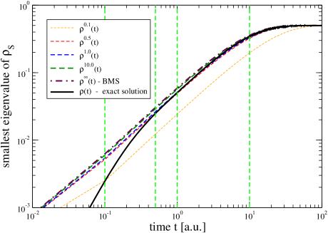
Figure 1: [Color Online] Eigenvalue evolution of the system density matrix (only one eigenvalue shown since trace-conservation implies a symmetric evolution) initialized in the pure state $\left<i\right|\rho_{\rm S}^{0}\left|j\right>=1/2$ for single-qubit dephasing. As predicted by Eqn. (99), the solutions of the coarse-graining master equations (thin dashed lines) intersect the exact solution (solid line) at $t=\tau$ (vertical dashed lines). The secular approximation (thick dashed line) corresponds to $\tau\to\infty$ and does not correctly cover the short time behavior of the exact solution. Parameters were chosen as follows: $\beta=1$, $\omega_{\rm ph}=1$, $\omega_{\rm ct}=5$, $s=1$, $\lambda=0.1$.

Note also that for large coarse graining times, figure 1 shows that the coarse-graining master equations approach the secular approximation master equation – which can also be seen as a numerical confirmation of Eqn. (27).

IV.3.2 Dissipative Coupling

With considering $A_{1}=\sigma^{x}$, an exponentially decaying correlation function (51), and $H_{\rm S}=\frac{1}{2}\left[\mbox{\boldmath$1$}-\sigma^{z}\right]$ one obtains a more complicated master equation for $\rho_{\rm S}^{\tau}(t)$ in the Schrödinger picture

$$\dot{\rho_{\rm S}^{\tau}}(t) = \left[\frac{i}{2}\sigma^{z}-i\sigma_{00}(\tau)\left|0\right>\left<0\right|-i\sigma_{11}(\tau)\left|1\right>\left<1\right|,\rho_{\rm S}^{\tau}\right]$$ (100)

$$+\gamma_{01,01}(\tau)\left[\left|0\right>\left<1\right|\rho_{\rm S}^{\tau}\left|1\right>\left<0\right|-\frac{1}{2}\left\{\left|1\right>\left<1\right|,\rho_{\rm S}^{\tau}\right\}\right]$$

$$+\gamma_{10,10}(\tau)\left[\left|1\right>\left<0\right|\rho_{\rm S}^{\tau}\left|0\right>\left<1\right|-\frac{1}{2}\left\{\left|0\right>\left<0\right|,\rho_{\rm S}^{\tau}\right\}\right]$$

$$+\gamma_{01,10}(\tau)\left|0\right>\left<1\right|\rho_{\rm S}^{\tau}\left|0\right>\left<1\right|$$

$$+\gamma_{10,01}(\tau)\left|1\right>\left<0\right|\rho_{\rm S}^{\tau}\left|1\right>\left<0\right|\,.$$

From the non-vanishing matrix elements in Eqn. (24) one can deduce that (unlike in the pure dephasing case) the Lamb-shift term will contribute, since (although diagonal) it is not proportional to the identity matrix anymore. Likewise, we also observe here a decoupled evolution of diagonal

$${\rho_{\rm S}^{\tau}}_{00}(t) = \frac{\gamma_{01,01}}{\gamma_{01,01}+\gamma_{10,10}}\left[1-e^{-\left(\gamma_{01,01}+\gamma_{10,10}\right)t}\right]$$ (101)

$$+e^{-\left(\gamma_{01,01}+\gamma_{10,10}\right)t}{\rho_{\rm S}^{\tau}}_{00}(0)$$

and off-diagonal matrix elements

$${\dot{\rho_{\rm S}}^{\tau}}_{01} = \left[i-\Gamma(\tau)\right]{\rho_{\rm S}^{\tau}}_{01}+\gamma_{01,10}(\tau)\left({\rho_{\rm S}^{\tau}}_{01}\right)^{*}\,,$$ (102)

with $\Gamma(\tau)=\frac{1}{2}\left(\gamma_{01,01}+\gamma_{10,10}\right)-i\left(\sigma_{11}-\sigma_{00}\right)$ (we have omitted the $\tau$-dependence). Considering even and odd Fourier transforms of the form (52) corresponding to exponentially decaying correlation functions, we can now compare the solution (86) of the Born equation with the solutions (100) of the coarse-graining approach.

When one initializes the density matrix as $\rho_{\rm S}(0)=\left|0\right>\left<0\right|$ one finds that for infinite coarse-graining times the diagonal terms will equilibrate to value 1/2 (which corresponds to thermalization at infinite temperatures), see figure 2.

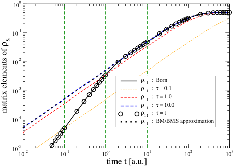
Figure 2: [Color Online] Evolution of the $\rho_{11}$-matrix element of the density matrix for dissipative coupling. The solid line represents the solution of the Born Eqn. (86) and the thin dashed lines correspond to solutions of (100) for different coarse graining times $\tau$. Up to second order in $\lambda$, a perfect numerical agreement is found for the matrix elements of $\rho^{t}(t)$ (symbols) and the Born solution (solid line). Parameters were chosen as follows: $\lambda=0.1$, $\tau_{\rm b}=1$.

In this case, the off-diagonal terms will evidently vanish throughout. Note that for the small coupling chosen ($\lambda=0.1$), the solution of the Born equation $\rho_{\rm S}(t)$ is approximated by the adaptive coarse-graining solutions $\rho_{\rm S}^{t}(t)$ with extraordinary accuracy.

In contrast, when initializing the density matrix as $\rho_{\rm S}(0)=\frac{1}{2}\left[\left|0\right>\left<0\right|+\left|0\right>\left<1\right|+\left|1\right>\left<0\right|+\left|1\right>\left<1\right|\right]$ one observes that the diagonal entries will remain unchanged and the off-diagonals will decay. The actual behavior of the decay of the off-diagonal elements is depicted in figure 3.

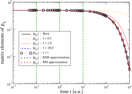
Figure 3: [Color Online] Evolution of the ${\left|\rho_{01}\right|}$ matrix element of the density matrix for pure dissipation. The solid line represents the solution of the Born Eqn. (86) and the thin dashed lines correspond to solutions of (100) for different coarse graining times $\tau$. Up to second order in $\lambda$, a perfect agreement is found for the matrix elements of $\rho^{t}(t)$ (symbols) and the Born solution (solid line). The difference between Born solution and BM as well as BMS approximations is too small to be visible. Parameters were chosen as follows: $\lambda=0.1$, $\tau_{\rm b}=1$.

Again we observe a strikingly good agreement between the Born solution $\rho_{\rm S}(t)$ and the adaptive coarse-graining solutions $\rho_{\rm S}^{t}(t)$.

It is also instructive to compare for the adaptive coarse-graining approach the limit of infinite coarse-graining times (BMS approximation)

$$\dot{\rho_{\rm S}} = \left(\frac{i}{2}+\frac{i}{2}\frac{\lambda^{2}\tau_{\rm b}}{1+\tau_{\rm b}^{2}}\right)\left[\sigma^{z},\rho_{\rm S}\right]$$

$$+\frac{\lambda^{2}}{1+\tau_{\rm b}^{2}}\left[\left|0\right>\left<1\right|\rho_{\rm S}\left|1\right>\left<0\right|+\left|1\right>\left<0\right|\rho_{\rm S}\left|0\right>\left<1\right|-\rho_{\rm S}\right]$$

with the BM approximation master equation (64), where one can see that only the equations for the diagonals match. Likewise, in the limit $\tau_{\rm b}\to 0$ one obtains

$$\dot{\rho_{\rm S}^{\tau}} = \frac{i}{2}\left[\sigma^{z},\rho_{\rm S}^{\tau}\right]$$ (104)

$$+\lambda^{2}\left[\left|0\right>\left<1\right|\rho_{\rm S}^{\tau}\left|1\right>\left<0\right|+\left|1\right>\left<0\right|\rho_{\rm S}^{\tau}\left|0\right>\left<1\right|-\rho_{\rm S}^{\tau}\right]$$

$$+\lambda^{2}e^{-i\tau}{\rm sinc}\left[\tau\right]\left|0\right>\left<1\right|\rho_{\rm S}^{\tau}\left|0\right>\left<1\right|$$

$$+\lambda^{2}e^{+i\tau}{\rm sinc}\left[\tau\right]\left|1\right>\left<0\right|\rho_{\rm S}^{\tau}\left|1\right>\left<0\right|\,.$$

Here, one finds that the BMS approximation ($\tau\to\infty$) yields a different master equation than the BM limit (62) and also the BM approximation (64) However, also within the coarse-graining approach the limit $\tau_{\rm b}\to 0$ (with finite $\tau$) leads to the same steady state as the BMS approximation $\tau\to\infty$ and the BM limit (62) – only the relaxation rates may differ. Note however that the BM approximation (64) may even lead to instable behavior of the off-diagonal matrix elements for large $\lambda$ (compare also section IV.4), whereas the coarse-graining approach always generates Lindblad forms.

IV.3.3 General Coupling

For a more complex coupling of the spin to the reservoir

$$H_{\rm S}=\frac{1}{2}\left[\mbox{\boldmath$1$}-\sigma^{z}\right]\,,\qquad\vec{n}_{1}=\frac{1}{\sqrt{2}}(1+i,1+i,1+i)\,,$$ (105)

and also more realistic spectral coupling densities of type (47) we find thermalization as predicted by the BMS approximation for long times. For short times however, the solution $\rho_{\rm S}^{t}(t)$ may strongly differ from the BMS solution, see figure 4.

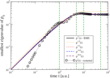
Figure 4: [Color Online] Evolution of the eigenvalues of the density matrix for a single qubit initialized in the pure state $\left<i\right|\rho_{\rm S}^{0}\left|j\right>=1/2$. For long times the BMS solution (thick dashed line) and the adaptive coarse-graining solution (thick solid line) predict thermalization in the thermal equilibrium state (15), whereas a different equilibrium state is assumed for short coarse-graining times (thin dashed lines). Parameters were chosen as follows: $\beta=1$, $\omega_{\rm ph}=1$, $\omega_{\rm ct}=5$, $s=1$, $\lambda=0.1$.

For example, if coarse-graining times are chosen too small, a non-thermalized steady state is obtained. For large coarse-graining times, the thermalized steady state is reached, but then in the short time regime, large differences between fixed graining and the adaptive graining solution are found. Again, we numerically confirm Eqn. (27), since for large coarse graining times the secular approximation is reproduced.

IV.4 Staying Reasonable

Frequently, the BM approximation (12) is used although it does not generally guarantee for positive evolution. This is certainly tolerable if the solution obtained approximates the exact solution well (and thus violates positivity only slightly). In addition, if the interaction Hamiltonian used in such models implicitly corresponds to a secular approximation childs2001 ; schuetzhold2005a , one will obtain a Lindblad form master equation and positivity as well as stability of the density matrix will be granted throughout. In general however, this will not be the case. Here we will analytically consider a single qubit $H_{\rm S}=\frac{1}{2}\left[\mbox{\boldmath$1$}-\sigma^{z}\right]$ with the simple coupling $H_{\rm SB}=\sigma^{x}\otimes B$. Denoting with $\Gamma(\omega)$ the half-sided Fourier-transform (11) of the reservoir correlation function, one can write Eqn. (12) in the form $\dot{\rho_{\rm S}}=L\rho_{\rm S}(t)$ and calculate the eigenvalues of the Liouvillian.

If one is only interested in the subspace of diagonal density matrices one finds the two corresponding eigenvalues $\sigma_{0}=0$ and $\sigma_{1}=-2\lambda^{2}A$ with $A=\Re\left\{\Gamma(+1)+\Gamma(-1)\right\}$. For physically motivated bath correlation functions $C_{11}$ in Eqn. (IV.1.1) one obtains that $\sigma_{1}<0$, such that the evolution in this subspace may not lead to unstable behavior – although positivity may be violated.

In contrast, in the off-diagonal subspace one obtains the two eigenvalues $\lambda_{2/3}=-2\lambda^{2}A\pm\sqrt{-1+2B\lambda^{2}+A^{2}\lambda^{4}}$ with $A$ defined as above and $B=\Im\left\{\Gamma(-1)-\Gamma(+1)\right\}$. Given $B>0$ (which can be achieved with correlation functions of form (IV.1.1)), one of these will pick a positive real part as soon as $\lambda^{2}>(2B)^{-1}$, which corresponds to an unstable evolution, see also figure 5. Numerically, we observe the same for $n=2$ mutually uncoupled qubits (with similar system Hamiltonians and couplings). In this case, the expectation value of operators that are not diagonal in the system Hamiltonian will not yield any meaningful results and the Born-Markov approximation is questionable.

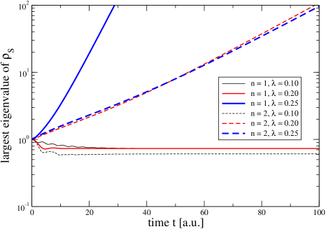
Figure 5: [Color Online] Largest eigenvalue of the density matrix for one (solid) and two (dashed) qubits initialized with $\left<i\right|\rho_{\rm S}^{0}\left|j\right>=1/2^{n}$. calculated from Eqn. (12). For large $\lambda$, not only positivity is violated (negative eigenvalues not shown – trace conservation), but the solution even becomes unstable. The parameters in (IV.1.1) were chosen as $\beta=1$, $\omega_{\rm ph}=1$, $\omega_{\rm ct}=5$, $s=2$, such that the transition from stable to unstable behavior occurs at $\lambda_{\rm crit}\approx 0.231294$ for $n=1$.

IV.5 Thermalization

In the pure dephasing limit, one observes a rapid (i.e., exponential) decay of the off-diagonal elements of the density matrix. Also, if there are no degeneracies in the spectrum, the rotating wave approximation (III.2) predicts a decoupled evolution of the diagonal elements of the density matrix in the eigenbasis of $H_{\rm S}$, i.e., from the corresponding evolution equation $\dot{\rho}_{ii}(t)=\sum_{j}A_{ij}\rho_{jj}(t)$ one might expect an exponential decay into the eigenvector of the matrix $A$ which has eigenvalue 0 (steady state). The corresponding subspace can still be degenerate (many stationary states) or there may exist exponentially many other eigenvectors with very small eigenvalues, such that thermalization does not necessarily happen very fast. Here we will consider some specific realizations of the spin-boson model (35) and solve Eqn. (III.2) numerically.

For example, if the system Hamiltonian has degeneracies and the coupling to the reservoir does not lift these, the system may relax into states that are not even diagonal in the system Hamiltonian basis. In these cases, the initial density matrix may determine which steady state is actually reached, see figure 6. As a first example we consider

$$\gamma=1\,,\qquad\gamma^{z}_{1}=\gamma^{z}_{2}=-\frac{1}{2}\,,$$

$$\vec{n}_{1}=\vec{n}_{2}=\frac{1}{\sqrt{2}}(1+i,1+i,1+i)\,,$$ (106)

and all other coefficients of Eqn. (35) vanishing, such that there exists a two-fold degeneracy in the spectrum of $H_{\rm S}$. In this subsection, we will consider spectral densities of type (47).

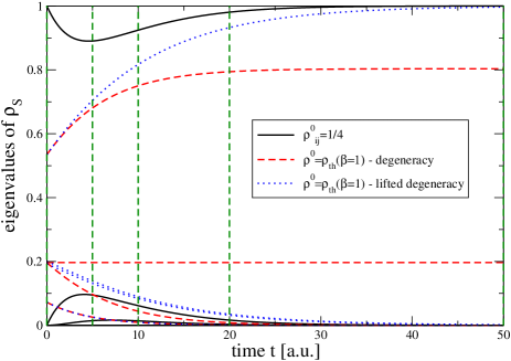
Figure 6: [Color Online] Top: Eigenvalue evolution for a 2-qubit system according to the secular approximation master Eqn. (III.2) with a two-fold degeneracy for different initial states (solid and dashed lines) and with a near two-fold degeneracy (dotted lines). Vertical dashed lines indicate the times at which the bottom row snapshots have been taken.
Bottom rows: Absolute values of the matrix elements of the corresponding $4\times 4$ density matrix in the ordered energy eigenbasis (such that the top left corner corresponds to the ground state). Color coding ranges from blue (value 0) to red (value 1). In the upper row, the system is initialized in a non-thermal density matrix $\left<i\right|\rho_{\rm S}^{0}\left|j\right>=1/4$ and relaxes into a the thermalized state (15) with $\beta_{\rm sys}=\beta$, i.e., for the low reservoir temperature chosen ($\beta=10$) essentially into the ground state. In contrast, in the middle row the initial state was a thermalized one with initial system temperature $\beta^{0}_{\rm sys}=1$, and the system does not relax into a thermal equilibrium state. In the lowest row, the degeneracy was broken by choosing $\gamma^{z}_{1}=-1/2+0.01$ and $\gamma^{z}_{2}=-1/2-0.01$.
Other parameters were chosen as $\beta=10$, $\omega_{\rm ph}=1$, $\omega_{\rm ct}=5$, $s=1$, $\lambda=0.1$.

For the low reservoir temperatures assumed in figure 6, thermalization corresponds to relaxation into the ground state and one can see that it may depend on the initial state of the density matrix and possibly lifted degeneracies whether thermalization takes place. In reality, the degeneracy might always be lifted by some imperfect Hamiltonian implementations. In addition, the coupling to the reservoir may be more complex than in (IV.5) thus making the thermalized system state (15) the only stationary state of the rotating wave master Eqn. (III.2), compare also breuer2002 . However, it is to be expected that thermalization in this case will take rather long times, especially for large and complicated systems (see next subsection).

IV.6 Solving Problems by Cooling

It is known that Hamiltonians of the form (35) can be used to encode solutions to computationally hard problems in their ground state. This is for example exploited in adiabatic quantum computation farhi2001a . For a system made of five spins, we will compare an enlarged version of the previous example (IV.5)

$$\gamma=\frac{5}{2}\,,\qquad\gamma^{z}_{i=1..5}=-\frac{1}{2}$$ (107)

with the ground state encoding of Exact Cover 3 – a specific NP-complete problem.

The Exact Cover 3 problem can be introduced as follows farhi2001a : Given a set of $m$ constraints where each constraint contains the positions of three bits $C_{m}=(p^{1}_{m},p^{2}_{m},p^{3}_{m})$ (with evidently $1\leq p^{i}_{m}\leq n$), one is looking for the $n$-bit bit-string $b_{1},\ldots,b_{n}$ (with $b_{i}\in\{0,1\}$) that fulfills for each constraint $b_{p^{1}_{m}}+b_{p^{2}_{m}}+b_{p^{3}_{m}}=1$ (where ”+” denotes the integer sum). One way to encode the solution to this problem into the ground state of a Hamiltonian of the type (35) is given by banuls2006a ; schuetzhold2006a

$$\gamma=m\,,\qquad\gamma^{z}_{i}=-\frac{n_{i}}{2}\,,\qquad\gamma^{zz}_{ij}=+\frac{n_{ij}}{2}$$ (108)

and all other coefficients vanishing – the differing pre-factor of $\gamma^{zz}_{ij}$ in comparison to schuetzhold2006a results from the absence of double-counting in $ij$ in Eqn. (35). In above equation, $m$ denotes the total number of clauses, $n_{i}$ the number of clauses involving bit $i$, and $n_{ij}$ the number of clauses involving both bits $i$ and $j$. Specifically, we will consider the 4 clauses $C_{1}=(2,3,4)$, $C_{2}=(1,2,5)$, $C_{3}=(1,4,5)$, and $C_{4}=(3,4,5)$. This implies the non-vanishing coefficients $\gamma=4$, $\gamma^{z}_{1}=\gamma^{z}_{2}=\gamma^{z}_{3}=-1$, $\gamma^{z}_{4}=\gamma^{z}_{5}=-3/2$, $\gamma^{zz}_{12}=\gamma^{zz}_{14}=\gamma^{zz}_{23}=\gamma^{zz}_{24}=\gamma^{zz}_{25}=\gamma^{zz}_{35}=1/2$, and $\gamma^{zz}_{15}=\gamma^{zz}_{34}=\gamma^{zz}_{45}=1$.

As can be easily checked, this problem has the unique solution $\left|10100\right>$ (with energy $E_{0}=0$) and the first excited states (with a six-fold degeneracy) are given by $\left|00101\right>,\left|10010\right>,\left|00001\right>,\left|00010\right>,\left|01001\right>,\left|01010\right>$ with energies $E_{1}=\ldots=E_{6}=1$. The first excited states have Hamming distances (i.e., number of bit-flips necessary for transformation) to the solution of $2,2,3,3,4,4$, respectively. This already indicates the hardness of such problems. Simple coupling Hamiltonians such as (37) that are only linear in the Pauli matrices will to first order only yield transitions between states with Hamming distance 1, since $\left<a\right|\sigma_{i}^{x/y}\left|b\right>=0$ if $\left|a\right>$ and $\left|b\right>$ have Hamming distance larger than one. Of course, this does not completely prohibit transitions between states with a larger Hamming distance, but such tunneling processes will have to pass through energetically less favorable states and are therefore strongly suppressed. Accordingly, one may expect that the process of thermalization is strongly hampered. This is also observed in figure 7, where we have assumed a reservoir temperature much smaller than the fundamental energy gap.

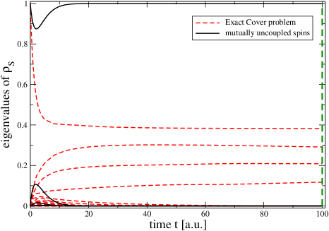
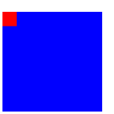
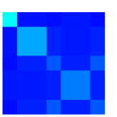
Figure 7: [Color Online] Top: Eigenvalue evolution for a 5-qubit system according to the secular approximation master Eqn. (III.2) for different system Hamiltonians given by Eqn. (107) (solid lines) and equation (108) with an Exact Cover 3-problem (dashed lines), respectively. In both cases, the density matrix has been initialized as $\left<i\right|\rho_{\rm S}^{0}\left|j\right>=1/32$. Whereas for the uncoupled spin system the system rapidly relaxes into the ground state, the final state for the exact cover problem is very different. Bottom: Absolute values of the matrix elements of the $7\times 7$ top left sub-matrix of the full $32\times 32$ density matrix in the ordered energy eigenbasis. On the left (corresponding to the solid line on top), the system relaxes to the ground state (red spot), whereas for the exact cover problem (right, dashed line on top), the system state is not thermalized.
Other parameters were chosen as $\beta=10$, $\omega_{\rm ph}=1$, $\omega_{\rm ct}=5$, $s=1$, $\lambda=0.1$.

Whereas for the simple qubit system (107) the system rapidly relaxes into the ground state, this is very different for the example (108).

V Conclusion

We have compared different procedures of deriving master equations from microscopic models and have shown that by using a coarse-graining approach one always obtains master equations in Lindblad form. This ensures for positivity and stability of the density matrix. In contrast, the usual Markovian approximation scheme may sometimes lead to a non-positive and even unstable behavior, where in the latter case there is no hope of approximating the exact solution. The coarse-grained master equations depend on a parameter – the coarse graining timescale $\tau$. For short coarse-graining times that are adaptively matched with the physical time, the solution $\rho_{\rm S}^{\tau}(\tau)$ must approximate the result of the Born-approximation by construction. For large coarse-graining times and time-independent system Hamiltonians, we reproduce the secular approximation. For all intermediate coarse-graining times, a positive evolution of the system density matrix is ensured by the Lindblad form of the resulting differential equations governing the time evolution. For the special case of pure dephasing of a single qubit we reproduce the analytical result by lidar2001a that $\rho_{\rm S}^{t}(t)=\rho_{\rm S}(t)$ yields the exact solution (which is of course equivalent in the weak-coupling limit to the Born approximation). For the simple example of exponentially decaying correlation functions we find by numerical simulation a surprisingly perfect agreement between solutions of the integro-differential Born equation and solutions of the adaptive coarse-graining approach. Given an interest in the system density matrix at time $t$, we therefore propose to match the coarse-graining time with the physical time $\tau=t$. In this case one has to calculate the Liouvillian matrix elements (III.3.1) only once (for the desired time $t$) and then evolve the density matrix using Eqn. (24) until that time $t$. In terms of computational complexity, this is more efficient than an evolving an integro-differential equation. A similar advantage is given when the resulting master equations are so simple such that an analytical solution in terms of the dampening matrix elements is possible. If in contrast the system is very complex and one is interested in the density matrix at all times, this advantage is destroyed. From a computational perspective, it would therefore be interesting to find the general map

$$\dot{\rho_{\rm S}}(t)={\cal L}(t)\rho_{\rm S}(t)=\lim_{\Delta t\to 0}\frac{\rho_{\rm S}(t+\Delta t)-\rho_{\rm S}(t)}{\Delta t}$$ (109)

which fulfills $\rho_{\rm S}(t)=\rho_{\rm S}^{t}(t)$. Formally, such a map can be found by inserting the solution $\rho_{\rm S}^{\tau}(t)=e^{L^{\tau}t}\rho_{\rm S}(0)$ into the derivative in Eqn. (109)

$${\cal L}(t) = \lim_{\Delta t\to 0}\frac{1}{\Delta t}\left[e^{L^{t+\Delta t}\cdot(t+\Delta t)}e^{-L^{t}\cdot t}-1\right]$$ (110)

$$= \left[\frac{d}{dt}e^{L^{t}\cdot t}\right]e^{-L^{t}\cdot t}\,.$$

We have given various examples of simple qubit systems coupled to a bosonic reservoir where thermalization which have demonstrated that thermalization of spin systems coupled to a bosonic bath may depend on a plethora of factors such as the initial state, complexity of the system Hamiltonian and complexity of the coupling. Future research will consider the importance of the coarse graining approach for different scenarios.

Appendix A Neglect of back-action

Throughout the paper, we make the following simplifying assumptions

Initial factorization of the density matrix:
By assuming

$$\mbox{\boldmath$\rho$}(0)=\mbox{\boldmath$\rho_{\rm S}$}(0)\otimes\mbox{\boldmath$\rho_{\rm B}^{0}$}=\rho_{\rm S}(0)\otimes\rho_{\rm B}^{0}$$ (111)

we implicitly demand that one can at $t=0$ prepare the system in a product state, which requires sufficient experimental control.

Born approximation:
For a bath much larger than the system and weak coupling it is reasonable to assume that the back-action of the system onto the bath is small, such that the bath part of the density matrix is hardly changed from its initial value, i.e.

$$\mbox{\boldmath$\rho$}(t^{\prime})=\mbox{\boldmath$\rho_{\rm S}$}(t^{\prime})\otimes\mbox{\boldmath$\rho_{\rm B}^{0}$}+{\cal O}\{\lambda\}\,.$$ (112)

Clearly, inserting this approximation in the third term in (7) is consistent up to second order in $\lambda$.

Reservoir in Stationary State:
We will assume that the reservoir is in a stationary state of the bath Hamiltonian, which implies $\left[\mbox{\boldmath$\rho_{\rm B}^{0}$},H_{\rm B}\right]=0$. One possibility of such a stationary state is to assume the thermal equilibrium state ($\beta^{-1}=k_{\rm B}T$ at temperature $T$)

$$\mbox{\boldmath$\rho_{\rm B}^{0}$}=\rho_{\rm B}^{0}=\frac{e^{-\beta H_{\rm B}}}{{\rm Tr_{B}}\left\{e^{-\beta H_{\rm B}}\right\}}\,.$$ (113)

Appendix B Markov Approximation

Starting from the Born Eqn. (8), the Markovian approximation in breuer2002 is performed by replacing (in the interaction picture) $\mbox{\boldmath$\rho_{\rm S}$}(t^{\prime})\to\mbox{\boldmath$\rho_{\rm S}$}(t)$ under the integral, substituting $\tau=t-t^{\prime}$ and extending the integration to infinity. This is usually motivated by fastly decaying reservoir correlation functions (9). By doing so, we obtain the BM Master Equation

$$\dot{\rho_{\rm S}} = -i{\rm Tr_{B}}\left\{\left[\mbox{\boldmath$H_{\rm SB}$}(t),\mbox{\boldmath$\rho_{\rm S}$}(0)\mbox{\boldmath$\rho_{\rm B}^{0}$}\right]\right\}$$ (114)

$$-\int\limits_{0}^{\infty}{\rm Tr_{B}}\left\{\left[\mbox{\boldmath$H_{\rm SB}$}(t),\left[\mbox{\boldmath$H_{\rm SB}$}(t-\tau),\mbox{\boldmath$\rho_{\rm S}$}(t)\mbox{\boldmath$\rho_{\rm B}^{0}$}\right]\right]\right\}d\tau$$

$$+{\cal O}\{\lambda^{3}\}\,,$$

where one can now insert the decomposition (2) of the interaction Hamiltonian to obtain

$$\dot{\rho_{\rm S}} = -i\lambda\sum_{\cal A}\left<B_{\cal A}\right>\left[\mbox{\boldmath$A_{\cal A}$}(t),\mbox{\boldmath$\rho_{\rm S}$}(0)\right]$$ (115)

$$+\lambda^{2}\Big{\{}\sum_{\cal AB}\int\limits_{0}^{\infty}\left[\mbox{\boldmath$A_{\cal B}$}(t-\tau)\mbox{\boldmath$\rho_{\rm S}$}(t),\mbox{\boldmath$A_{\cal A}$}(t)\right]C_{\cal AB}(\tau)d\tau$$

$$+{\rm h.c.}\Big{\}}+{\cal O}\left\{\lambda^{3}\right\}\,,$$

with the reservoir correlation functions (9). We will use $\left<B_{\cal A}\right>=0$ throughout, since this case can always be generated with a suitable transformation trafo . In order to evaluate the time-dependence of the operators in (115), it is useful to expand them into eigenoperators of the system Hamiltonian (assuming $H_{\rm S}$ to be time-independent)

$$A_{\cal A} = \sum_{\omega}A_{\cal A}(\omega)=\sum_{\omega}A_{\cal A}^{\dagger}(\omega)=A_{\cal A}^{\dagger}\,,$$

$$A_{\cal A}(\omega) = \sum_{ab}\delta_{(E_{b}-E_{a}),\omega}\left|a\right>\left<a\right|A_{\cal A}\left|b\right>\left<b\right|\,,$$ (116)

where the variable $\omega$ ranges over all energy differences of $H_{\rm S}$, $H_{\rm S}\left|a\right>=E_{a}\left|a\right>$ and $\delta$ is a Kronecker symbol. These operators $A_{\cal A}(\omega)$ have the advantageous properties

$$\left[H_{\rm S},A_{\cal A}(\omega)\right] = -\omega A_{\cal A}(\omega)\,,$$

$$\left[H_{\rm S},A_{\cal A}^{\dagger}(\omega)\right] = +\omega A_{\cal A}^{\dagger}(\omega)\,,$$

$$\left[H_{\rm S},A_{\cal A}^{\dagger}(\omega)A_{\cal B}(\omega)\right] = 0\,,$$ (117)

which implies in the interaction picture

$$\mbox{\boldmath$A_{\cal A}$}(t)=\sum_{\omega}e^{-i\omega t}A_{\cal A}(\omega)=\sum_{\omega}e^{+i\omega t}A_{\cal A}^{\dagger}(\omega)\,.$$ (118)

With inserting the half-sided Fourier transform of the reservoir correlation functions (11) we obtain for the master equation in (115) with $\left<B_{\cal A}\right>=0$

$$\dot{\rho_{\rm S}} \approx \lambda^{2}\Big{\{}\sum_{\cal AB}\sum_{\omega,\omega^{\prime}}e^{i(\omega^{\prime}-\omega)t}\Gamma_{\cal AB}(\omega)\left[A_{\cal B}(\omega)\mbox{\boldmath$\rho_{\rm S}$}(t),A_{\cal A}^{\dagger}(\omega^{\prime})\right]$$ (119)

$$+{\rm h.c.}\Big{\}}\,.$$

Finally, we observe that by re-inserting the definition of the eigenoperators (B) in (119) and switching back to the Schrödinger picture the time-dependent phase factors vanish and one obtains the Born-Markov master Eqn. (12).

Appendix C Secular approximation

For large times, the terms with an oscillating prefactor in Eqn. (119) will average out and by inserting

$$e^{i(\omega^{\prime}-\omega)t}\mbox{\boldmath$\rho_{\rm S}$}(t)\approx\delta_{\omega,\omega^{\prime}}\mbox{\boldmath$\rho_{\rm S}$}(t)$$ (120)

in Eqn. (119) and switching to the Schrödinger picture (compare also e.g. chapter 3.3 in breuer2002 ) we obtain

$$\dot{\rho_{\rm S}} = -i\left[H_{\rm S},\rho_{\rm S}(t)\right]$$

$$+\lambda^{2}\sum_{\omega}\sum_{\cal AB}\left\{\Gamma_{\cal AB}(\omega)\left[A_{\cal B}(\omega)\rho_{\rm S},A_{\cal A}^{\dagger}(\omega)\right]+{\rm h.c.}\right\}\,.$$

The advantage of the secular approximation is that we can now combine the half sided Fourier transforms to full (even and odd) Fourier transforms (III.2) of the reservoir correlation functions. Inserting these definitions into (C), one obtains a Lindblad lindblad1976a form

$$\dot{\rho_{\rm S}} = -i\left[H_{\rm S},\rho_{\rm S}(t)\right]$$

$$-i\left[\frac{\lambda^{2}}{2i}\sum_{\omega}\sum_{\cal AB}\sigma_{\cal AB}(\omega)A_{\cal A}^{\dagger}(\omega)A_{\cal B}(\omega),\rho_{\rm S}(t)\right]$$

$$+\lambda^{2}\sum_{\omega}\sum_{\cal AB}\gamma_{\cal AB}(\omega)\times$$

$$\times\left[A_{\cal B}(\omega)\rho_{\rm S}A_{\cal A}^{\dagger}(\omega)-\frac{1}{2}\left\{A_{\cal A}^{\dagger}(\omega)A_{\cal B}(\omega),\rho_{\rm S}(t)\right\}\right]\,,$$

where the positivity of the $\gamma_{\cal AB}(\omega)$-matrix is guaranteed by Bochners theorem breuer2002 ; alicki1987 , which states that the Fourier transform of a function of positive type (as are the reservoir correlation functions) gives rise to a positive definite matrix. In above equation, the second commutator corresponds to the unitary action of decoherence (Lamb-shift). Finally, we can insert the operator definitions (B) in (C) to obtain Eqn. (III.2). Naturally, if $\left[H_{\rm S},A_{\cal A}\right]=0$ (pure dephasing), BM and BMS approximations are equivalent.

Appendix D Adiabatic approximation

With inserting the ansatz

$$U(t) = \sum_{ab}u_{ab}(t)\exp\left\{-i\int\limits_{0}^{t}E_{\alpha}(t^{\prime})dt^{\prime}\right\}\times$$ (123)

$$\times\left|a(t)\right>\left<b(0)\right|\,,$$

where the $\left|a(t)\right>$ span an instantaneous basis (chosen to be complete and orthonormal) of the system Hilbert space defined via $H_{\rm S}(t)\left|a(t)\right>=E_{a}(t)\left|a(t)\right>$ in the evolution equation for the time evolution operator $\dot{U}(t)=-iH_{\rm S}(t)U(t)$, one obtains an equation for the expansion coefficients

$$\dot{u}_{ab}+u_{ab}\left<a|\dot{a}\right>=-\sum_{c\neq a}u_{cb}e^{-i\int\limits_{0}^{t}g_{ca}(t^{\prime})dt^{\prime}}\left<a|\dot{c}\right>$$

with the energy gap

$$g_{ca}(t^{\prime})=E_{c}(t^{\prime})-E_{a}(t^{\prime}).$$ (125)

With introducing the Berry phase sun1988a

$$\gamma_{a}(t)=i\int\limits_{0}^{t}\left<a(t^{\prime})|\dot{a}(t^{\prime})\right>dt^{\prime}$$ (126)

this can also be written as

$$\frac{d}{dt}\left(u_{ab}e^{-i\gamma_{a}(t)}\right) = -\sum_{c\neq a}u_{cb}e^{-i\gamma_{a}(t)-i\int\limits_{0}^{t}g_{ca}(t^{\prime})dt^{\prime}}\left<a|\dot{c}\right>\,,$$

which gives the general time evolution of the expansion coefficients $u_{ab}$ for any (also non-adiabatic) system Hamiltonian $H_{\rm S}(t)$ if one uses the initial condition $u_{ab}(0)=\delta_{ab}$. The full adiabatic approximation essentially consists in setting the right hand side of above equation to zero: For slowly varying system Hamiltonians, the change of the eigenvectors will be negligible such that $\left<a|\dot{c}\right>\approx 0$. Note however, that in the vicinity of avoided crossings, the condition of adiabaticity relates the maximum speed of the time evolution with the spectral properties of the system Hamiltonian

$$\left<a|\dot{c}\right>=\frac{\left<a\right|\dot{H_{\rm S}}\left|c\right>}{E_{c}-E_{a}}\,,$$ (127)

see also e.g. jansen2007a ; schaller2006b . If $\left<a|\dot{c}\right>\approx 0$, one obtains with the adiabatic approximation $u_{ab}^{\rm ad}(t)=\delta_{ab}e^{i\gamma_{a}(t)}$ which implies for the time evolution operator in the adiabatic limit

$$U(t) \approx \sum_{a}e^{i\gamma_{a}(t)-i\int\limits_{0}^{t}E_{a}(\tau)d\tau}\left|a(t)\right>\left<a(0)\right|\,.$$ (128)

Therefore, we obtain for the time-averaged operator in (III.4)

$${\left<\left<\mbox{\boldmath$\tilde{A}_{\cal A}$}(\omega)\right>\right>}_{[t,t+\tau]} \approx \sum_{ab}\left|a(0)\right>\left<b(0)\right|\times$$

$$\times\frac{1}{\tau}\int\limits_{t}^{t+\tau}\left<a(t^{\prime})\right|A_{\cal A}\left|b(t^{\prime})\right>\times$$

$$\times e^{-i\left[\gamma_{ab}(t^{\prime})-\omega t^{\prime}-\int\limits_{0}^{t^{\prime}}g_{ab}(\tau)d\tau\right]}dt^{\prime}$$

with $\gamma_{ab}(t^{\prime})=\gamma_{a}(t^{\prime})-\gamma_{b}(t^{\prime})$ and $g_{ab}(\tau)=E_{a}(\tau)-E_{b}(\tau)$.

Appendix E Positivity-preserving master equations

Here we will show that master equations of the form

$$\dot{\rho} = -i\left[{\cal H}(t),\rho(t)\right]$$ (130)

$$+\sum_{\alpha\beta=1}^{K}\Gamma_{\alpha\beta}(t)\Big{[}{\cal L}_{\alpha}(t)\rho(t){\cal L}_{\beta}^{\dagger}(t)$$

$$-\frac{1}{2}\left\{{\cal L}_{\beta}^{\dagger}(t){\cal L}_{\alpha}(t),\rho(t)\right\}\Big{]}$$

generally preserve the positive semidefiniteness of an initial condition $\rho(0)$ if the matrix $\Gamma_{\alpha\beta}(t)$ is positive semidefinite and the operator ${\cal H}(t)={\cal H}^{\dagger}(t)$ is hermitian at all times (smoothness of all time-dependencies provided). With discretizing the time derivative and by introducing new operators

$$W_{1}(t) = \mbox{\boldmath$1$}=W_{1}^{\dagger}(t)\,,$$

$$W_{2}(t) = i{\cal H}(t)+\frac{1}{2}\sum_{\alpha\beta}\Gamma_{\alpha\beta}(t){\cal L}_{\beta}^{\dagger}(t){\cal L}_{\alpha}(t)\,,$$

$$W_{3}(t) = {\cal L}_{1}(t)\,,$$

$$\vdots$$

$$W_{K+2}(t) = {\cal L}_{K}(t)$$ (131)

we obtain

$$\rho(t+\Delta t)=\sum_{\alpha\beta=1}^{K+2}w_{\alpha\beta}(t)W_{\alpha}(t)\rho(t)W_{\beta}^{\dagger}(t)$$ (132)

where the $w_{\alpha\beta}(t)$ matrix is given by

$$w(t)=\left(\begin{array}[]{cc|c}1&-\Delta t&0\cdots 0\\ -\Delta t&0&0\cdots 0\\ \hline\cr 0&0&\\ \vdots&\vdots&\Delta t\Gamma(t)\\ 0&0\end{array}\right).$$ (138)

This matrix has a simple block structure and it is therefore straightforward to relate the eigenvalues of $w$ to those of $\Gamma$. In particular, one obtains the eigenvalues $w_{1}=1/2\left[1-\sqrt{1+4\Delta t^{2}}\right]$, $w_{2}=1/2\left[1+\sqrt{1+4\Delta t^{2}}\right]$, and $w_{i\geq 3}(t)=\Delta t\gamma_{i-2}(t)$, where $\gamma_{i-2}(t)$ are the non-negative eigenvalues of $\Gamma(t)$. With diagonalizing the matrix in (132) via $w_{\alpha\beta}(t)=\sum_{\gamma}u_{\alpha\gamma}(t)u_{\beta\gamma}^{*}(t)w_{\gamma}(t)$ with a suitable (time-dependent) unitary transformation $U(t)$ we obtain from Eqn. (132)

$$\rho(t+\Delta t) = \sum_{\gamma}w_{\gamma}(t)\tilde{W}_{\gamma}(t)\rho(t)\tilde{W}_{\gamma}^{\dagger}(t)\,,$$

$$\tilde{W}_{\gamma}(t) = \sum_{\alpha}u_{\alpha\gamma}(t)W_{\alpha}(t)\,.$$ (139)

Assuming that at time $t$ we have a valid density matrix with $0\leq\rho_{\delta}(t)\leq 1$ we obtain by inserting the spectral decomposition $\rho(t)=\sum_{\delta}\rho_{\delta}(t)\left|\Phi_{\delta}(t)\right>\left<\Phi_{\delta}(t)\right|$

$$\left<\Phi\right|\rho(t+\Delta t)\left|\Phi\right> = \sum_{\gamma\delta}w_{\gamma}(t)\rho_{\delta}(t){\left|\left<\Phi\right|\tilde{W}_{\gamma}\left|\Phi_{\delta}(t)\right>\right|}^{2}$$ (140)

$$\geq \frac{1}{2}\left[1-\sqrt{1+4\Delta t^{2}}\right]\times$$

$$\times\sum_{\delta}\rho_{\delta}(t){\left|\left<\Phi\right|\tilde{W}_{1}\left|\Phi_{\delta}(t)\right>\right|}^{2}$$

$$\geq -\Delta t^{2}\sum_{\delta}\rho_{\delta}(t){\left|\left<\Phi\right|\tilde{W}_{1}\left|\Phi_{\delta}(t)\right>\right|}^{2}$$

$$\stackrel{{\scriptstyle\Delta t\to 0}}{{\geq}} 0\,,$$

such that in the limit $\Delta t\to 0$ (which defines the original differential Eqn. (130)), the smallest eigenvalue of the density matrix at time $t+\Delta t$ approaches zero faster than the discretization width $\Delta t$. Therefore, in this limit the matrix $w(t)$ becomes positive semidefinite and the differential Eqn. (132) becomes a positivity-preserving map.

Appendix F Sinc Distribution

For discrete $a,b$ and continuous $\omega$ we would like to analyze

$$f(\omega,a,b) \equiv \lim_{\tau\to\infty}\tau\;{\rm sinc}\left[(\omega+a)\frac{\tau}{2}\right]{\rm sinc}\left[(\omega+b)\frac{\tau}{2}\right]$$ (141)

$$= \lim_{\tau\to\infty}\frac{4\sin\left[(\omega+a)\frac{\tau}{2}\right]\sin\left[(\omega+b)\frac{\tau}{2}\right]}{(\omega+a)(\omega+b)\tau}\,.$$

One can consider the case $a\neq b$ by a partial fraction expansion where without loss of generality we find for the first term (due to the symmetry the second term can be treated in a completely analogous way)

$$I_{a\neq b} = \int\limits_{-\infty}^{+\infty}g(\omega)\frac{\sin\left[(\omega+a)\frac{\tau}{2}\right]\sin\left[(\omega+b)\frac{\tau}{2}\right]}{\tau(\omega+a)}d\omega$$

$$= \cos\left[(b-a)\frac{\tau}{2}\right]\int\limits_{-\infty}^{+\infty}g(\omega)\frac{\sin^{2}\left[(\omega+a)\frac{\tau}{2}\right]}{\tau(\omega+a)}d\omega$$

$$+\frac{1}{2}\sin\left[(b-a)\frac{\tau}{2}\right]\int\limits_{-\infty}^{+\infty}g(\omega)\frac{\sin\left[(\omega+a)\tau\right]}{\tau(\omega+a)}d\omega\,,$$

where we have inserted $(\omega+b)=(\omega+a)+(b-a)$ to use trigonometric relations for $\sin(\alpha+\beta)$. With a suitable transformation, this becomes

$$I_{a\neq b} = \frac{\cos\left[(b-a)\frac{\tau}{2}\right]}{\tau}\int\limits_{-\infty}^{+\infty}g\left(\frac{x}{\tau}-a\right)\frac{\sin^{2}(x/2)}{x}dx$$ (142)

$$+\frac{\sin\left[(b-a)\frac{\tau}{2}\right]}{2\tau}\int\limits_{-\infty}^{+\infty}g\left(\frac{x}{\tau}-a\right)\frac{\sin(x)}{x}dx\,,$$

where for large $\tau$, the dominant integral contribution evaluates the (smooth) function $g(\omega)$ near $g(-a)$ such that this value can be taken out of the integral and we obtain $\lim\limits_{\tau\to\infty}I_{a\neq b}=0$. Using the representation

$$\lim\limits_{\tau\to\infty}\tau\,{\rm sinc}^{2}\left[\Omega\tau\right]=\pi\delta(\Omega)$$ (143)

one can consider the general case via

$$f(\omega,a,b) \asymp \delta_{ab}\lim_{\tau\to\infty}\tau\;{\rm sinc}^{2}\left[(w+a)\frac{\tau}{2}\right]$$ (144)

$$= \delta_{ab}\pi\delta\left(\frac{w+a}{2}\right)\,,$$

which yields Eqn. (27).

References

• (1) P. W. Shor, SIAM J. Comp. 5, 1484-1509, (1997).
• (2) L. K. Grover, Phys. Rev. Lett. 79, 325-328, (1997).
• (3) M. A. Nielsen and I. L. Chuang, Quantum Computation and Quantum Information, Cambridge University Press, Cambridge, (2000).
• (4) H.-P. Breuer and F. Petruccione, The Theory of Open Quantum Systems, Oxford University Press, Oxford, (2002).
• (5) V. Khidekel, Phys. Rev. E 52, 2510, (1995).
• (6) A. M. Childs, E. Farhi, and J Preskill, Phys. Rev. A 65, 012322, (2001).
• (7) E. Farhi et al., Science 292, 472-476, (2001).
• (8) M. S. Sarandy, L.-A. Wu, and D. A. Lidar, Quant. Inf. Proc. 3, 331-349, (2004).
• (9) S. Jansen, M. B. Ruskai, and R. Seiler, J. Math. Phys. 48, 102111, (2007).
• (10) G. Schaller, S. Mostame, and R. Schützhold, Phys. Rev. A 73, 062307, (2006).
• (11) M. H. S. Amin, P. J. Love, and C. J. S. Truncik, Phys. Rev. Lett. 100, 060503, (2008).
• (12) Y. Zhao and G. H. Chen, Phys. Rev. E 65, 056120, (2002).
• (13) S. Stenholm and M. Jakob, J. Mod. Opt. 51, 841-850, (2004).
• (14) P. Pechukas, Phys. Rev. Lett. 73, 1060, (1994); R. Alicki, ibid. 75, 3020, (1995); P. Pechukas, ibid. 75, 3021, (1995).
• (15) T. Yu, L. Diosi, N. Gisin, and W. T. Strunz, Phys. Lett. A 265, 331, (2000).
• (16) G. Lindblad, Commun. Math. Phys. 48, 119-130, (1976).
• (17) W. J. Munro and C. W. Gardiner, Phys. Rev. A 53, 2633 - 2640, (1996).
• (18) J. Wilkie, Phys. Rev. E 62, 8808 - 8810, (2000).
• (19) A. Tameshtit and J. E. Sipe, Phys. Rev. Lett. 77, 2600, (1996).
• (20) R. J. C. Spreeuw and T. W. Hijmans, Phys. Rev. A 76, 022306, (2007).
• (21) R. Karrlein and H. Grabert, Phys. Rev. E, 55, 153, (1997).
• (22) The general case $\left<B_{\cal A}\right>\neq 0$ can be reduced to the case $\left<B^{\prime}_{\cal A}\right>=0$ by using the transformations $H_{\rm S}\to H_{\rm S}^{\prime}=H_{\rm S}+\lambda g_{\cal A}\sum_{\cal A}A_{\cal A}$ and $B_{\cal A}\to B_{\cal A}^{\prime}=B_{\cal A}-g_{\cal A}\mbox{\boldmath$1$}$ in the Schrödinger picture, where the real constant has to be adapted such that $g_{\cal A}=\left<B_{\cal A}\right>$.
• (23) B. Vacchini, Phys. Rev. Lett. 84, 1374 - 1377, (2000).
• (24) D. A. Lidar and Z. Bihary and K. B. Whaley, Chem. Phys. 268, 35–53, (2001).
• (25) U. Kleinekathöfer, J. Chem. Phys. 121, 2505, (2004).
• (26) M. Schröder, M. Schreiber, and U. Kleinekathöfer, J. Chem. Phys. 126, 114102, (2007).
• (27) R. S. Whitney, J. Phys. A: Math. Theor. 41, 175304, (2008).
• (28) M. O. Scully and M. S. Zubairy, Quantum Optics, Cambridge University Press, Cambridge, (2002).
• (29) E. Anderson et al., LAPACK Users’ Guide, SIAM, (1999)
http://www.netlib.org/lapack.
• (30) W. H. Press et al., Numerical Recipes in C, Cambridge University Press, Cambridge, (1994).
• (31) T. Brandes and T. Vorrath, Phys. Rev. B 66, 075341, (2002); T. Brandes, Physics Reports 408, 315-474, (2005).
• (32) F.Nesi et al., Phys. Rev. B 76 155323, (2007); F. Nesi et al., Europhys. Lett. 80, 40005, (2007).
• (33) W. G. Unruh, Phys. Rev. A 51, 992-997, (1995).
• (34) G. Burkard, e-print:[cond-mat.mes-hall/0803.0564], (2008).
• (35) R. Schützhold and M. Tiersch, J. Opt. B: Quantum and Semiclassical Optics 7, 120-125, (2005).
• (36) M. C. Banuls et al., Phys. Rev. A 73, 022344, (2006).
• (37) R. Schützhold and G. Schaller, Phys. Rev. A 74, 060304(R), (2006).
• (38) R. Alicki and K. Lendi, Quantum Dynamical Semi-Groups and Applications, Lect. Notes Phys. 286, Springer-Verlag, Berlin, (1987).
• (39) C.-P. Sun, J. Phys. A: Mathematical and General 21, 1595-1599, (1988).