The coalescence of invariant manifolds and the spiral structure of barred galaxies

Abstract

In a previous paper (Voglis et al. 2006a, paper I) we demonstrated that, in a rotating galaxy with a strong bar, the unstable asymptotic manifolds of the short period family of unstable periodic orbits around the Lagrangian points L₁ or L₂ create correlations among the apocentric positions of many chaotic orbits, thus supporting a spiral structure beyond the bar. In the present paper we present evidence that the unstable manifolds of all the families of unstable periodic orbits near and beyond corotation contribute to the same phenomenon. Our results refer to a N-Body simulation, a number of drawbacks of which, as well as the reasons why these do not significantly affect the main results, are discussed. We explain the dynamical importance of the invariant manifolds as due to the fact that they produce a phenomenon of ‘stickiness’ slowing down the rate of chaotic escape in an otherwise non-compact region of the phase space. We find a stickiness time of order $100$ dynamical periods, which is sufficient to support a long-living spiral structure. Manifolds of different families become important at different ranges of values of the Jacobi constant. The projections of the manifolds of all the different families in the configuration space produce a pattern due to the ‘coalescence’ of the invariant manifolds. This follows closely the maxima of the observed $m=2$ component near and beyond corotation. Thus, the manifolds support both the outer edge of the bar and the spiral arms.

1 Introduction

The dynamics of spiral arms in rotating galaxies with a strong non-axisymmentric perturbation is probably very different from that in galaxies with a weak non-axisymmentric perturbation (see Contopoulos 2004 for a review). In the case of weak perturbation, bars or oval distortions have small, if not zero amplitude, and the main constituents of the non-axisymmetric component of the matter are the spiral arms themselves. The spirals are successfully described by models based on stable periodic orbits and the quasi-periodic orbits around them. Chaos is of little or no importance in such models. In the case of strong perturbation, on the other hand, the spirals start near the ends of strong bars, and they may extend to large distances beyond corotation. Furthermore, many orbits near and beyond corotation are chaotic, and some of them (the so called ‘hot population’ (Sparke and Sellwood 1987)) can wander both inside and outside corotation. In self-consistent models of barred spiral galaxies it has been indicated for the first time by Kaufmann and Contopoulos (1996) that these chaotic orbits play a significant role by supporting both the bar and the spiral arms. More recently, N-body models (Voglis et al. 2006b), or response models fitting a real barred spiral galaxy (Patsis 2006), were constructed in which the spiral arms are supported almost entirely by chaotic orbits.

To construct a theory of spiral structure based on orbits means essentially to provide a theoretical mechanism explaining how the angular positions of the apsides (apocenters) of the orbits become delineated in a way reproducing self-consistently an observed spiral pattern. In the case of weak perturbation, the alignment is produced by the stable periodic orbits of the $x_{1}$ family which form ‘precessing ellipses’, i.e., a family of ellipses with apocenters changing their azimuthal position, as a function of the Jacobi constant, in a direction along the spiral arms (see Grosbøl 1994 for a review). The termination of the main spiral is placed near the 4/1 resonance (Contopoulos 1985, Contopoulos and Grosbøl 1986, 1988, Patsis et al. 1991, 1994, Patsis and Kaufmann 1999), but weak extensions may also be found beyond the 4/1 resonance, reaching the corotation region.

However, these models are not applicable in the case of spirals in a galaxy with a strong bar, in which the orbits supporting the spiral are chaotic. Precisely, in our previous paper (Voglis et al. 2006a, hereafter paper I) we proposed a mechanism yielding the alignment of the apocenters of the chaotic orbits that is necessary in order to produce a spiral pattern. This is based on the invariant manifolds of the family of short period unstable periodic orbits which exist around the unstable equilibria $L_{1}$ or $L_{2}$. Besides our study, the role of these manifolds has been pointed out in the formation both of rings (Romero-Gomez et al. 2006) and spiral arms (Romero-Gomez et al. 2007).

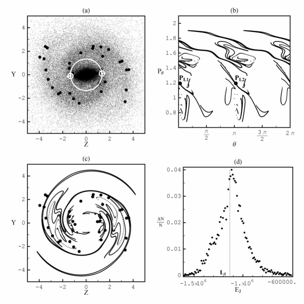
Figure 1: (a) A snapshot of the N-Body simulation (same as in Fig.5a of paper I). The thick dots show local maxima of the projected surface density. The big white circle passes through the unstable Lagrangian points $L_{1}$, $L_{2}$ and it is refered to as the corotation circle. The small circles around $L_{1}$ and $L_{2}$ are the short period unstable periodic orbits $PL_{1}$, $PL_{2}$. (b) Projection of the invariant manifolds of the $PL_{1}$ and $PL_{2}$ orbits in the surface of section $(\theta,p_{\theta})$, with $p_{r}=\dot{r}=0$ and $\dot{p}_{r}<0$ (condition of the apocenters), for the value of the Jacobi constant $E_{J}=-1.125\times 10^{6}$. (c) Projection of the same manifolds as in (b) in the configuration space $(y,z)$. The thick dots are the same as in (a). (d) The distribution of the values of the Jacobi constants of all the N-body particles which are in small bins $r\Delta r\Delta\theta$ around the maxima of the surface density, i.e., the thick dots of (a). The distribution is normalized according to the total number of particles in all the bins.

The basic paradigm for this mechanism is summarized in Figure 1. Keeping the same notation as in paper I, we deal with an N-Body system (Fig.1a) which is flat on the plane $(y,z)$, called the disk plane, and has also some thickness along the x-axis, vertical to the disk (details on the numerical runs and features of the system are given in subsection 2.1 below). Fig.1a shows the projection of the particles on the disk plane at the snapshot $t=47$ (after seven pattern rotations). The thick dots mark the positions of local maxima of the projected surface density, derived by counting the particles in successive rings from the center on the plane $(y,z)$. In the snapshot shown in Fig.1a the system has a strong bar as well as a conspicuous bi-symmetric spiral pattern which lies almost entirely outside corotation (marked by a white circle passing through $L_{1,2}$).

The small white circles in Fig.1a around $L_{1}$ and $L_{2}$ are orbits belonging to the family of short period unstable periodic orbits, which bifurcate from $L_{1}$ or $L_{2}$ and form loops around these points. The period of the loop is of the same order as the value of the epicyclic period at corotation. The family of these orbits, which are hereafter called $PL_{1}$ orbits (or $PL_{2}$, around $L_{2}$), exists for values of the Jacobi constant $E_{J}>E_{J,L_{1}}$. Here, as in paper I, we define the Jacobi constant by a 2D Hamiltonian approximation on the disk plane, namely

$$E_{J}={1\over 2}(v_{y}^{2}+v_{z}^{2})-\Omega_{p}(zv_{y}-yv_{z})+V(x=0,y,z)~{}~{}.$$ (1)

The potential function $V(x,y,z)$ is found from the N-Body code in a closed mathematical form expressed as a series of basis functions with coefficients calculated via a ‘smooth field’ technique (see subsection 2.1 below).

For a fixed value of $E_{J}$ there is one short period orbit, $PL_{1}$, around $L_{1}$ and the symmetric orbit $PL_{2}$ around $L_{2}$ (Fig.1a). Let $(r,p_{r})$, $(\theta,p_{\theta})$ be canonical pairs of variables in the Hamiltonian describing the orbits:

$$H(r,\theta,p_{r},p_{\theta})\equiv{1\over 2}\big{(}p_{r}^{2}+{p_{\theta}^{2}\over r^{2}}\big{)}-\Omega_{p}p_{\theta}+V(r,\theta)$$ (2)

where $V(r,\theta)\equiv V(x=0,r\sin\theta,r\cos\theta)$. The space of the variables $(r,\theta,p_{r},p_{\theta})$ is called the phase space. Let $r(t)$, $\theta(t)$, $p_{r}(t)$, $p_{\theta}(t)$ denote an orbit with initial conditions $(r_{0},\theta_{0},p_{r0},p_{\theta 0})$ under the time flow (time$=t$) of the Hamiltonian (2). The unstable manifold of $PL_{1}$ is defined as the set of initial conditions $(r_{0},\theta_{0},p_{r0},p_{\theta 0})$ in phase space tending asymptotically to $PL_{1}$ in the backward sense of time, namely

$${\cal W}^{U}_{PL_{1}}=\big{\{}\bigcup(r_{0},\theta_{0},p_{r0},p_{\theta 0}):\lim_{t\rightarrow-\infty}||Q(t;r_{0},\theta_{0},p_{r0},p_{\theta 0})-PL_{1}||=0\big{\}}$$ (3)

where $Q(t;r_{0},\theta_{0},p_{r0},p_{\theta 0})$ denotes the position of a particle in an orbit starting with the above initial conditions, and the norm $||\cdot||$ is defined as the minimum of the distances of $Q(t)$ from the locus of all the points in phase space belonging to the orbit $PL_{1}$. In the forward sense of time, the orbits with initial conditions taken on ${\cal W}^{U}_{PL_{1}}$ and near $PL_{1}$ deviate exponentially from $PL_{1}$ with a rate determined by the largest eigenvalue of the linearized flow around $PL_{1}$. However, the linearized approximation is not valid at large distances from $PL_{1}$ and the invariant manifold ${\cal W}^{U}_{PL_{1}}$ acquires in general a quite complicated form. In particular, the intersections of the unstable manifold ${\cal W}^{U}_{PL_{1}}$ with the stable manifold

$${\cal W}^{S}_{PL_{1}}=\big{\{}\bigcup(r_{0},\theta_{0},p_{r0},p_{\theta 0}):\lim_{t\rightarrow\infty}||Q(t;r_{0},\theta_{0},p_{r0},p_{\theta 0})-PL_{1}||=0\big{\}}$$ (4)

produce the so-called ‘homoclinic tangle’ which is the main source of chaos locally, in a domain of the phase space surrounding $PL_{1}$.

The unstable and stable manifolds ${\cal W}^{U}_{PL_{1}}$, ${\cal W}^{S}_{PL_{1}}$ are two-dimensional sets embedded in the three-dimensional hypersurface of fixed Jacobi constant. Let $p_{r}=\dot{r}=0$, $\dot{p}_{r}<0$ be the plane of the phase space corresponding to the set of points where orbits reach their apocenters. The intersection of ${\cal W}^{U}_{PL_{1}}$ with the plane $p_{r}=\dot{r}=0$ defines a one-dimensional set that we still call the unstable manifold of $PL_{1}$. Fig.1b shows the projection of the manifolds ${\cal W}^{U}_{PL_{1}}$ and ${\cal W}^{U}_{PL_{2}}$ in the plane $(\theta,p_{\theta})$. The plane $(\theta,p_{\theta})$ is hereafter called the surface of section. We clearly observe the intricate shape of the unstable invariant manifold that results in a strongly chaotic behavior of the orbits near $PL_{1}$ and $PL_{2}$. Fig.1c shows the projection of the same manifolds on the plane $(y=r\sin\theta,z=r\cos\theta)$, called the configuration space, which is the usual space where the motion of stars takes place. Although the projection of the invariant manifolds on the plane $(y,z)$ is rather intricate, it is clear that most of the time the manifolds follow closely the spiral pattern that is defined by the maxima of the particles’ surface density (a detailed comparison of the two patterns is made in section 3 below). In fact, every time when a chaotic orbit with initial conditions on these manifolds reaches an apocentric position, this position is always at another point of the same mamifolds. Thus, the apocenters of all the chaotic orbits of the manifold create an invariant locus as shown in Fig.1c. Hence, in paper I we supported that such manifolds yield, precisely, the necessary mechanism of alignment of the apocenters that induces the observed spiral pattern of the system.

Now, the manifolds shown in Figs.1b,c correspond to a particular value of the Jacobi constant $E_{J}=-1.125\times 10^{6}$ in the N-Body units introduced in paper I (summarized in subsection 2.1 below). However, the particles forming the spiral are spread in a wide range of values of the Jacobi constant. Figure 1d shows the distribution of Jacobi constants for the particles counted within small cells $r\Delta r\Delta\theta$, $\Delta r=0.2$, $\Delta\theta=\pi/26$, centered at the thick dots of Fig.1a, namely, along the spiral. The value $E_{J}=-1.125\times 10^{6}$ is very close to the peak of the distribution, but the distribution has a wide dispersion, of order $\sigma=5\times 10^{5}$. The one $\sigma$ level of the distribution is in the range $E_{J,min}\simeq-1.25\times 10^{6}$, $E_{J,max}\simeq-0.95\times 10^{6}$. This means that the manifolds shown in paper I correspond to a very narrow band of energies compared to the real distribution. Since many families of unstable periodic orbits coexist at different values of the Jacobi constant, the question is then whether the invariant manifolds of these families play also some role in the observed spiral pattern.

In the present paper we consider the invariant manifolds of many different periodic orbits covering a significant part of the range of Jacobi constants in the histogram of Fig.1d. Let us note that the $PL_{1,2}$ family, i.e., the only family examined in paper I, does not exist for values of the Jacobi constant $E_{J}<E_{J,L_{1}}=-1.133\times 10^{6}$, whereas Fig.1d clearly shows that about half of the mass in this histogram is in particles with $E_{J}<E_{J,L_{1}}$. Thus, for these particles it is necessary to consider the invariant manifolds of families other than $PL_{1}$ in order to complete the picture of paper I. But even when we considered the domain $E_{J}\geq E_{J,L_{1}}$, permissible to $PL_{1}$, we found that the invariant manifolds of other families play a role in determining the dynamics of chaotic orbits and, thereby, the spiral structure. In particular, we found that the invariant manifolds of all the examined families of unstable periodic orbits produce essentially the same pattern in configuration space, i.e., the same spiral pattern. These manifolds produce a phenomenon of ‘stickiness’, namely while the phase space is, in general, open to fast chaotic escapes (with escape times of only a few radial periods), the chaotic orbits with initial conditions on or close to an invariant manifold can only escape by following this manifold, and then the escape time increases considerably, i.e., it is of order $10^{2}$ periods. During this time the chaotic orbits support the spiral pattern. In fact, while many different families of periodic orbits co-exist at one value of the Jacobi constant, we find that only a subset of them create the dominant stickiness phenomena at that particular value. As analyzed below, the above phenomena can be explained on the basis of known properties of the invariant manifolds in conservative dynamical systems. When applied to the manifolds of the periodic orbits of the galaxy, these properties allow us to construct a consistent picture of the mechanism causing the alignment of the apocenters of the chaotic orbits along the spiral arms.

The paper is structured as follows: Section 2 describes briefly the simulation as well as the phase space structure of the system under study at various values of the Jacobi constant. This is compared to the distribution of the real particles of the N-body simulation. Section 3 presents the analysis of the invariant manifolds for nine different families of periodic orbits. Plots are given of the unstable manifolds of these orbits in phase space as well as in configuration space, which are compared with the distribution of the N-Body particles in both spaces. The observed spiral pattern is reconstructed by superposing these plots. We finally explore which families are dynamically important at various ranges of values of the Jacobi constant. Section 4 summarizes the main conclusions of the present study.

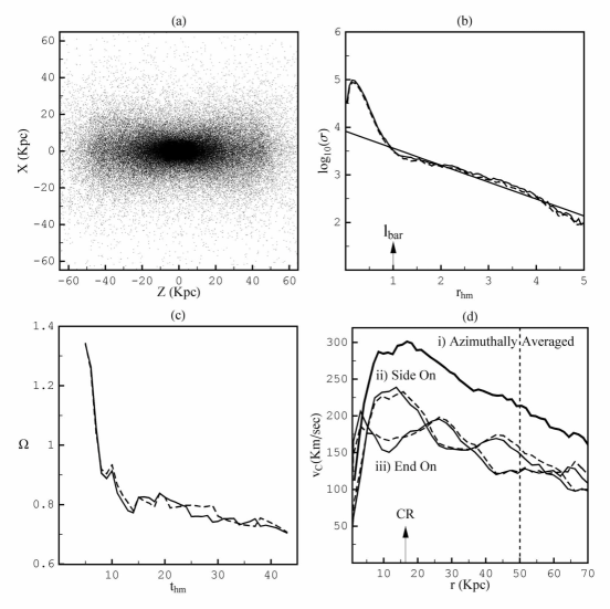
Figure 2: (a) The N-body system viewed edge-on (bar nearly line-on). (b) The projected surface density profile on the disk plane (y-z) for the experiment with $1.3\times 10^{5}$ particles (solid line) versus the same profile for the disk particles of the experiment with $1.17\times 10^{6}$ particles (dashed line). The straight solid line is an exponential fit to the surface density profile for the radii $r\geq l_{bar}=1$ (see text).(c) Comparison of the time evolution of the pattern speed, and (d) comparison of the rotation curves for the two experiments (solid lines = experiment with $1.3\times 10^{5}$ particles, dashed lines = experiment with $1.17\times 10^{6}$ particles). The top bold solid curve is the ‘azimuthally averaged’ rotation curve $v_{c}(r)=<L(r)>/r$ where $<L(r)>$ is the mean angular momentum perpendicularly to the disc for the particles in annuli of mean radius $r$ (see text).

2 Simulation and phase space structure

2.1 The N-Body experiment

The details of the numerical simulation have been presented in Voglis et al. (2006b). A brief account follows below.

Our analysis refers to a particular simulation called ‘QR3’ in Voglis et al. (2006b). This experiment starts with a triaxial equilibrium system which has initially no rotation. This system is obtained by running a ’collapse’ simulation. The particles are initially taken to have small radial position and velocity perturbations from an ideal Hubble flow. These perturbations correspond to a rms radial profile of mass perurbations in the early Universe of the form $\delta\mu/\mu\propto r^{-(n+3)/2}$, where the power exponent $n$, derived from the spectrum of density perturbations at decoupling, has the value $n=-2$ for perturbations corresponding to the galactic mass scale (fixed as $10^{12}$ solar masses). The initial positions and velocities of the particles are determined using the analytical formulae of Palmer and Voglis (1983) which yield practically equivalent results to the Zel’dovich (1970) approximation (a detailed description of the methodology of production of this type of initial conditions is given in sect. 3 of Efthymiopoulos and Voglis 2001). The numerical simulation starts well before the bound system has reached its maximum expansion, before collapsing. The initial redshift depends somewhat on the used value of the Hubble parameter but it is well before $z=10$. Thus, the Universe at the starting point of the simulation is to a great precision Einstein-de Sitter, even if the cosmological constant $\Lambda$ is non-zero. Furthermore, the system is considered isolated from its environment, thus the expansion of the Universe does not affect it any longer, i.e., the system is simulated by Newtonian forces (accelerations due to $\Lambda$ can be safely ignored at the galactic scale , e.g. in our galaxy $g_{\Lambda}/g_{gravity}\sim 10^{-5}\times(r/8Kpc)^{2}$). Thus, the above initial conditions are consistent with both an Einstein-de Sitter or $\Lambda$CDM model of the Universe with $\Omega=1$.

The violent relaxation phase is simulated using the tree code of Hernquist (1987), while the subsequent slow approach to equilibrium, through ‘phase mixing’, is simulated by an improved version of the self-consistent field (SCF) code of Allen et al. (1990). The equilibrium system is triaxial, and quite elongated, as a result of the onset of a radial orbit instability (the mean ellipticity on the plane of long and short axes is E6). Axes are oriented so that $z$ coincides with the long axis, $y$ with the intermediate axis, and $x$ with the small axis of the moment of inertia ellipsoid.

The triaxial equilibrium system serves as the basis for the production of a sequence of rotating systems which preserve the energy and virial equilibrium, but have different amounts of total angular momentum, i.e., different spin parameters $\lambda$. The detailed procedure by which rotation is added is described in section 2 of Voglis et al (2006b). It essentially consists of re-orienting, at a particular moment, the component $\vec{v}_{yz}$ of the velocity of each particle on the y-z plane so that the new vector $\vec{v}_{yz}^{\prime}$ has equal size as $\vec{v}_{yz}$ and is directed perpendicularly to the particle’s position vector $\vec{r}$ with respect to the center of mass of the system. By repeatedly implementing the velocity re-orientation procedure, after a system is allowed to relax for 20 half-mass crossing times at each step, we obtain a sequence of systems with progressively higher spin parameter.

The QR3 system is third in this sequence (with spin parameter $\lambda=0.22$). As in paper I, in the present paper we present results from a realization of the experiment using $1.3\times 10^{5}$ particles. However, as demonstrated below the features of the system remain practically invariant when the simulation is repeated using nine times as many particles ($1.17\times 10^{6}$).

We fix units by considering that the system contains a total mass equal to $M=10^{12}$ solar masses. The unit of length is the half-mass radius of the relaxed triaxial system at the begining of the simulation. For a Hubble parameter $H_{0}=72$Km/sec/Mpc, this turns out to be $R_{hm}=12.6$Kpc in physical units. The unit time is set equal to the half-mass crossing time $t_{hm}$ which in physical units is equal to 32Myr. The unit of velocity is, thus, $V_{unit}=0.48$Km/sec, while the unit of energy (per unit mass) is taken as $E_{unit}=V_{unit}^{2}$. Finally, the unit of angular momentum is taken equal to the value of the angular momentum for a circular orbit at corotation, $L_{unit}=\Omega_{p}R_{c}^{2}$. In all subsequent plots we use the above units (except for figs.2a,d in which we use physical units). The length unit must be rescaled by a factor $M^{1/2}/10^{6}$ if the mass is not equal to the adopted value $10^{12}$.

The morphological details of the QR3 experiment are given in section 3 of Voglis et al. (2006b). The main features of the system can be summarized as follows: The particles have no a priori identities as of belonging to a disk or a halo. The system is flattened as a whole, and when viewed edge on it yields an axial ratio $\sim 0.3$ (Fig.2a) (this was called a ‘thick disk’ in Voglis et al. 2006b). On the other hand, particles forming a thin disk can be identified by taking any small arbitrary value of the half-thickness $\Delta x$. We then find that there are particles which remain confined within a vertical distance $\Delta x$ from the equatorial plane during the whole simulation up to $t=47$. By varying $\Delta x$ the number of particles found to satisfy this criterion also varies. Adopting a conventional ratio of the disk over halo mass in a galaxy $M_{disk}/M_{halo}=1:5=0.2$, we vary $\Delta x$ until getting the value for which the percentage of particles staying confined to $\pm\Delta x$ becomes equal to $0.2$. Doing so, we found $\Delta x=0.145R_{hm}\simeq 2.2$Kpc. In the sequel we conventionally identify these particles as belonging to the disk, while the remaining particles are identified as halo particles. Such a distinction is a shortcoming of the simulation, since there is no a priori guarantee that the particles confined so far in the so-defined ‘disk’ do not escape from it at subsequent time steps. A better analysis would necessitate running separately the disk and halo particles, as in many standard simulations in the literature. One main reason for the present type of simulation, however, is the possibility to use an SCF code to produce the potential, so that the analysis of the phase space structure is possible in terms of smooth orbits.

In the simulation with $1.17\times 10^{6}$ particles we have about $2.3\times 10^{5}$ particles in the disk. The surface density profile $\sigma(R)$ of these particles (Fig.2b) compares very well with the projected surface density profile of the whole configuration in the simulation with $1.3\times 10^{5}$ particles. Thus, in both cases the projected surface density shows asymptotically (for large $r$) an exponential profile $\sigma(r)\propto\exp(-r/R_{D})$ with a scale length $R_{D}\simeq 0.82R_{hm}=10.3$Kpc. Taking the optical radius as $R_{0}\simeq 3R_{D}\simeq 31$Kpc, the disk thickness ratio is $2.2/31\simeq 0.07$.

The time evolution of the pattern speed $\Omega_{p}(t)$ is also quite similar in the simulations with $10^{5}$ and $10^{6}$ particles (Fig.2c). There is initially some angular deceleration which slows down considerably after a time $t=10t_{hm}$. At the snapshot $t=47$ (corresponding to $t=1.5$Gyr in physical units) the pattern speed is almost stabilized at a value $\Omega_{p}=0.67/t_{hm}$ or $\Omega_{p}=20.6$Km/sec/Kpc. The pattern has performed about seven revolutions by that time. The length of the major semi-axis of the bar can be estimated from the inner point (arrow of fig.2b) at which the profile $\sigma(R)$ starts deviating from exponential. We find $l_{bar}\sim 1R_{hm}=12.6$Kpc. Corotation (taken as the average of the distances to $L_{1}$ and $L_{4}$ is at $R_{c}\simeq 1.3\times l_{bar}=16.4$Kpc. Thus we have a strong, relatively slow and long bar which is reminiscent of the bars found in old and strongly barred galaxies (see e.g. Lindblad et al. 1996 for indicative values of the same parameters in the case of NGC1365, or Aguerri et al. (1998), Gadotti and de Souza (2006) and Michel-Dansac and Wozniak (2006) for more general references). In fact, the above given values for $l_{bar}$ and $R_{c}$ are somewhat larger than typical, but they should all be rescaled to smaller values if $M<10^{12}$.

The rotation curves obtained by calculating the mean values of the line-of-sight velocity profiles of the particles when the system is viewed edge-on and the bar is either side-on or end-on are shown in Fig.2d. The bold curve on top of the two other curves represents an ‘azimuthally averaged’ rotation curve, obtained via $v_{c}(r)=<L(r)>/r$, where $<L(r)>$ is the mean component of the angular momentum perpendicularly to the disk of all the particles in an annulus $r\pm\Delta r/2$ divided by the central radius of the annulus $r$. This calculation is the same as in Voglis et al. 2006b, fig.3e, but now it is given for the snapshot $t=47$. The horizontal axis is also in the same limits as in that figure. We notice that the azimuthally averaged rotation curve is declining, and the decline becomes Keplerian after a radius $R=\sim 3.2R_{c}=4R_{hm}=50$Kpc. This is due to the fact that the numerical code imposes a truncation radius for the whole system, i.e. the disk and the halo, after which Laplace’s equation is solved instead of Poisson’s equation. Nevertheless, the decline below this radius is less steep and the system partly mimics the effects of a disk embedded in a halo. More precisely, the peak value is at 300Km/sec and the value at 50Kpc is 220Km/sec. Thus, the decline is 27%. This picture is again reminiscent of strongly barred galaxies like NGC3515 (see the rotation curve in Lindblad et al. 1996). Similar conclusions are drawn by inspecting the rotation curves obtained by the line-of-sight velocity profiles. Since such profiles are biased towards their left wing, the rotational velocities obtained from then are smaller than those obtained by the azimuthal averaging. The difference increases as the velocity dispersion increases, and in our case it is of order 50Km/sec. In particular, the peak value of the side-on curve is at $v_{c}=250$Km/sec while the curve stabilizes at about a 35% lower value at $R=1.5R_{c}$ and remains flat up to about $1.2R_{o}=40$Kpc, where $R_{o}=3.2R_{D}$ is the disk’s optical radius. All our plots below of the configuration space are in square boxes of dimension $5R_{hm}=63$Kpc, thus, phenomena near the edge of these boxes are not so reliable. However, this does not affect in any essential way the behavior of the invariant manifolds well below this distance.

Another unpleasant feature of the simulation is the high velocity dispersion of the disk beyond the bar, with dispersions exceeding $100$Km/sec. This is due to the fact that the simulation is purely dissipationless, i.e., there are no gas effects simulated. Thus, both the disk and the halo become ’hot’ quickly. While this does not prevent us from detecting spiral $m=2$ components beyond the bar, the high value of the velocity dispersion causes the space between the spirals and the bar to be substabtially populated, while in observed galaxies this space often appears to be empty.

Finally, the amplitude of the spiral pattern undergoes oscillations during the whole run. This is an interesting phenomenon which is described in detail in subsection 2.5 of Voglis et al. 2006b. Up to $t=50$ the ratio $A_{2}/A_{0}$ of the Fourier decomposition of the surface density profile exhibits variations. The bar maximum is about $0.8$. On the other hand, the $A_{2}/A_{0}$ ratio for the spiral arms oscillates, roughly between the limits 0.2 and 0.5. The frequency of this oscillation is resonant with the bar. In fact, there appear to be two oscillating modes of the spiral pattern. An inner part, near $L_{1}$ or $L_{2}$, rotates almost together with the bar. An outer part (beyond $r=4$ length units) rotates more slowly than the bar. As a result, the two parts appear sometimes disjoint, and at other times they are rejoined. At snapshots when the two parts are joined smoothly, the whole spiral pattern becomes conspicuous, i.e., the amplitude $A_{2}/A_{0}$ becomes maximal over a large radial extent. The snapshots $t=18$, $t=47$ and $t=74$, treated in Paper I, are close to such a maximum. At such snapshots we typically find that the invariant manifolds trace well the spiral arms in a considerable part of the manifolds length. Although the above description renders immediately clear that there is more to consider in the dynamics of the spiral arms than simply the invariant manifolds, it is also clear that the latter are a key ingredient of the dynamics. This is further explored in the sequel.

2.2 Particle distribution and phase space structure

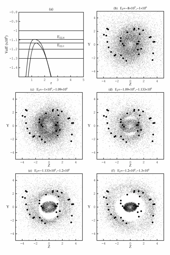
Figure 3: (a) Radial profiles of the effective potential $V_{eff}(R)=V(R,\theta_{fixed})+\Omega^{2}R^{2}/2$ along the directions $\theta_{fixed}$ pointing to $L_{1}$ (curve with lower maximum) and $L_{4}$ (curve with upper maximum). The five horizontal lines denote the levels of the Jacobi constant to which panels (b) through (f) refer. These panels show the distribution on the disk plane of the particles with Jacobi constants belonging to the intervals (b) $-8\times 10^{5}\geq E_{J}\geq-10^{6}$, (c) $-10^{6}\geq E_{J}\geq-1.09\times 10^{6}=E_{J,L4}$, (d) $E_{J,L4}=-1.09\times 10^{6}>E_{J}\geq-1.133\times 10^{6}=E_{J,L1}$, (e) $E_{J,L_{1}}=-1.133\times 10^{6}>E_{J}\geq-1.2\times 10^{6}$, and (f) $-1.2\times 10^{6}>E_{J}\geq-1.3\times 10^{6}$. The dots are the same as in Fig.1a.

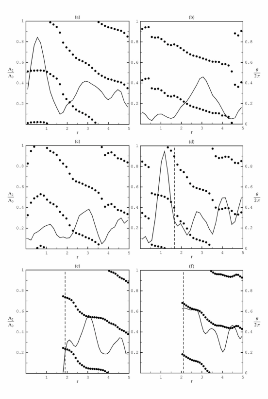
Figure 4: The ratio $A_{2}/A_{0}$ (solid lines) of the Fourier amplitudes $m=2$ vs. axisymmetric of the surface density $\Sigma(r,\theta)=\Delta N/(r\Delta r\Delta\theta)$, as a function of $r$, for the particles of (a) the whole simulation, and (b) to (f) the bins of Figs. 3b to 3f respectively. The black dots show the values of $\theta_{max}/2\pi$, as a function of $r$, where $\theta_{max}$ is an angle of maximum of the $m=2$ component for given $r$. The vertical dashed lines show the limits of $r$ beyond which annuli of central radius $r$ do not intersect the zero velocity curves of the effective potential for the lower values of the Jacobi constant indicated in the panels of Fig.3d to 3f respectively. In panels e and f the Fourier analysis refers only to the particles restricted to move outside corotation by the zero velocity curves.

Figures 3b to 3f show the distribution of the N-Body particles in the configuration space for five different bins of the energy (Jacobi constant) centered at the level values shown in Fig.3a (the radial profiles of the effective potential $V+\Omega^{2}R^{2}/2$ along the directions crossing $L_{1}$ and $L_{4}$ are superposed). The first bin $=-8\times 10^{5}\geq E_{J}\geq-10^{6}$ (Fig.3b) corresponds to particles with Jacobi constants well above both $E_{J,L_{1}}=-1.133\times 10^{6}$ and $E_{J,L4}=-1.09\times 10^{6}$. In the next bin (Fig.3c) the particles have Jacobi constants just above $E_{J,L4}$, i.e., $-10^{6}\geq E_{J}\geq E_{J,L4}$. In Fig.3d the particles have Jacobi constants between $E_{J,L4}$ and $E_{J,L1}$. The remaining two bins (Figs.3e,f) show the particles with Jacobi constants just below $E_{J,L1}$ ($E_{J,L_{1}}\geq E_{J}>-1.2\times 10^{6}$, Fig.3e) and well below it ($-1.2\times 10^{6}\geq E_{J}\geq-1.3\times 10^{6}$, Fig.3f) respectively. These energy bins cover an appreciable range of energies of the histogram of Fig.1a. The thick dots in panels 3b to 3f are the same as in Fig.1c. The following are observed:

a) The spiral structure is developed mostly by the particles of Fig.3d, i.e., in the energy bin $E_{J,L1}\leq E_{J}\leq E_{J,L4}$, i.e., in the corotation region.

b) Particles with $E_{J}<E_{J,L1}$ (Figs.3e,f) contribute to extensions of the spiral pattern well beyond corotation.

c) Particles with $E_{J}>E_{J,L_{4}}$ partly support the spiral pattern close to $L_{1,2}$ (Fig.3b,c), and partly contribute to the axisymmetric background. It should be noticed that the distribution of Fig.1d is obtained by counting all the particles which are inside bins $r\Delta r\Delta\theta$ at which the projected surface density presents local maxima. Thus, this distribution contains particles belonging to the spiral arms as well as to the axisymmetric background and it is actually impossible to distinguish these two components by the N-Body data.

A quantitative estimate of the importance of the spiral arms in the various bins of Figure 3 is obtained in Figure 4, which shows the profiles of the ratio $A_{2}/A_{0}$ (amplitude of the $m=2$ mode over the axisymmetric background), as a function of the radial distance $r$, from the Fourier analysis of the projected surface density $\Sigma(r,\theta)=\Delta N/(r\Delta r\Delta\theta)$ for the total N-Body simulation and for the separate bins of Figs.3b to 3f. In each panel of Fig.4, the left vertical axis yields values of the ratio $A_{2}/A_{0}$, and the dependence of this ratio on $r$ is shown by a solid curve. On the other hand, the right vertical axis in the same panels shows values of the azimuth $\theta$ normalized over $2\pi$, and the black dots denote the angles of the maxima of the $m=2$ mode, again as a function of $r$.

In Fig.4a, these quantities are shown for the surface density of Fig.1a, i.e., for the whole N-body experiment. The initial rise of the profile $A_{2}/A_{0}$ up to about $r=0.8$ corresponds to the bar $m=2$ amplitude, which reaches a peak value 0.8. After that, the value of $A_{2}/A_{0}$ declines to a minimum $A_{2}/A_{0}\simeq 0.1$ at $r=1.6$, but then it starts rising again, reaching a second maximum $A_{2}/A_{0}\simeq 0.4$ at $r=3$. In the whole region from $r=1.5$ to $r=4$ the angles of $m=2$ maxima $\theta_{max}(r)$ depend monotonically on $r$, and such a dependence defines spiral arms. After $r=4$ there is a second local maximum of $A_{2}/A_{0}$ which roughly corresponds to the outer spiral arms described in subsection 2.1.

The remaining panels (Figs.4b to 4f) show the same quantities for the particles in the corresponding panels of Fig.3. The main observation here is that the central bin $E_{J,L1}\leq E_{J}\leq E_{J,L4}$ (Fig.3d) contributes mostly to the $A_{2}/A_{0}$ amplitude at radii near corotation, i.e., immediately after the bar ($1\leq r\leq 2$, Fig.4d). In particular, very close to the unstable Lagrangian points (at $r=1.3$) the $A_{2}/A_{0}$ ratio approaches unity, and then it falls rather abruptly to a value fluctuating around $A_{2}/A_{0}=0.3$. On the other hand, in the remaining panels 4b,c,e, and f the amplitude $A_{2}/A_{0}$ becomes important after $r=2$. It should be noticed that a high value of $A_{2}/A_{0}$ (like 0.6 in Fig.4f) only means that the $m=2$ perturbation is relatively more important with respect to the axisymmetric background of the particles in the same bin (which are, however, fewer than the particles in the central bin $E_{J,L1}\leq E_{J}\leq E_{J,L4}$, see the histogram of Fig.1d). Furthermore, in the bins of Figs.4d,e,f, which correspond to values of the energy $E_{J}<E_{J,L4}$, we must take care of the fact that the motion of the particles is restricted either inside or outside corotation by the zero velocity curves (zvc) of the effective potential. Now, because of the presence of the bar, these curves are elliptically distorted with respect to perfect circles. Thus, when one makes the Fourier analysis of the surface density function within different annuli of width $\Delta r$, if an annulus intersects an inner or an outer limiting zvc at four bins ($\theta_{i}\pm\Delta\theta/2$) around respective values $\theta_{i}$, $i=1,2,3,4$, there are two symmetric intervals of the azimuth $\theta$ within which the annulus contains no bodies. This effect appears as an enhanced amplitude of the m=2 mode in the Fourier spectrum of $\Delta N(\theta)$ for such an annulus, with the m=2 maxima being either aligned or at right angles with the bar’s major axis. Thus, this effect is easily distinguished from a real m=2 mode due to spiral arms. The vertical dashed lines in the panels of Fig.4d,e,f mark the minimum values of $r$ beyond which annuli of central radius $r$ do not intersect the zero velocity curves of the effective potential for the lower values of the Jacobi constant indicated in the panels of Fig.3d to 3f respectively. In all cases we find significant $m=2$ amplitudes implying that the spiral arms are present in all the bins.

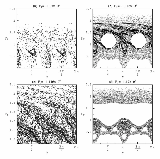
Figure 5: The phase portrait (surface of section $(\theta,p_{\theta})$, with $p_{r}=\dot{r}=0$ and $\dot{p}_{r}<0$ ) when (a) $E_{J}=-1.05\times 10^{6}$, (b and c) $E_{J}=-1.116\times 10^{6}$, and (d) $E_{J}=-1.17\times 10^{6}$. (c) is a magnification of (b) in the range of angular momenta $1.45\leq p_{\theta}\leq 2.1$. The manifolds in (b) are produced by the 7-th iterates of 10000 initial conditions along a small segment of length $DS=10^{-4}$ in the ustable eigendirection of the monodromy matrix at $PL_{1}$. In (c) the 8-th iterates of the same manifolds are plotted. The gray thick dots in (b) correspond to the projection of the locus of maxima of the spiral pattern (black dots of Fig.1a) on the surface of section corresponding to a constant energy $E_{J}=-1.116\times 10^{6}$.

Figure 5 shows the phase plots (surfaces of section $(\theta,p_{\theta})$) for three values of the Jacobi constant, namely $E_{J}=-1.05\times 10^{6}$ (Fig.5a, $E_{J}>E_{J,L4}$), $E_{J}=-1.116\times 10^{6}$ (Fig.5b,c $E_{J,L1}<E_{J}<E_{J,L4}$, and $E_{J}=-1.17\times 10^{6}$ (Fig.5d, $E_{J}<E_{J,L1}$). These plots are obtained by integrating the orbits of many test particles with initial conditions covering the entire plotted domain.

When $E_{J}>E_{J,L4}$ (Fig.5a) the phase space is open to escapes and, indeed, we find that for most initial conditions the orbits escape quickly, typically after less than 10 iterates (= 10 radial periods). Our numerical criterion for escapes is when an orbit crosses the radius $r=10r_{corotation}$. In fact, transport from inside to outside corotation (and vice versa) is energetically permissible at this value of the Jacobi constant, and we find numerically that the transport is fast even for orbits with very low initial values of $p_{\theta}$, which are placed initially inside the bar. Nevertheless, some chaotic orbits are also observed in Fig.5a which are ‘sticky’ to a chain of small islands of stability corresponing to a 4:1 commensurability. These particles remain trapped for longer times, which are typically of order $10^{2}$ periods. The patterns formed in the surface of section $(\theta,p_{\theta})$ by these particles have the typical form encountered in the so-called outer stickiness zones of the islands of stability in simple symplectic mappings (Efthymiopoulos et al. 1997). These zones are produced by the invariant manifolds of unstable periodic orbits of high multiplicity which are located near the main cantori marking the limits of the islands of stability. The cantori are invariant sets of points which represent the limit of a sequence of periodic orbits of progressively higher multiplicity which exist near the last KAM torus around an island of stability. A cantorus contains gaps through which chaotic transport is possible. The main sticky zone of any island is inside a cantorus with small gaps. The stickiness is caused by the limited flux allowed through the gaps. This is because the manifolds of the unstable periodic orbits near the cantorus develop a large number of oscilations in a direction almost parallel to the cantorus, thus creating a partial barrier to motions transversely to the cantorus. However, there can still be appreciable stickiness in a zone outside the cantorus, caused by the invariant manifolds of unstable periodic orbits located within that zone (Contopoulos and Harsoula 2007).

When $E_{J}$ is taken inside the interval $E_{J,L1}<E_{J}<E_{J,L4}$ (Fig.5b), the picture of the phase space portrait changes dramatically. Transport from inside to outside corotation is still energetically permissible within this interval of values of the Jacobi constant. Furthermore, the phase space is still open to escapes. However, as observed in Fig.5b, escapes are now much more difficult, and there is an inner domain (for $p_{\theta}<2$)which is almost uniformly covered by the iterates of chaotic orbits. This domain surrounds two roughly circular domains which are energetically prohibited to the motion. The inner limit of the large chaotic domain is defined by a rotational KAM curve, at values of $p_{\theta}$ close to and below $p_{\theta}=0.4$. The regular orbits below this curve correspond to quasi-periodic motions inside the bar. On the other hand, for high values of $p_{\theta}$ ($p_{\theta}>2$), the orbits in the chaotic domain of Fig.5b exhibit, again, a sticky behavior. Plotting the unstable invariant manifolds of the $PL_{1}$ and $PL_{2}$ orbits in the same figure shows that the stickiness zone is essentially defined by the outer parts of these manifolds. A magnification in this region (Fig.5c) clearly shows that the stickiness zone is structured by the invariant manifolds, i.e., the stickiness is more pronounced in those domains which are more densely covered by different parts of the invariant manifolds. A detailed study of this phenomenon, namely the structuring of the stickiness zone by invariant manifolds, was made in a simple dynamical system by Contopoulos and Harsoula (2007).

Now, the gray thick dots in Fig.5b yield the projection on the plane $(\theta,p_{\theta})$ of the locus of maxima of the spiral pattern of Fig. 1a. This is found by solving Eq.(2) for $p_{\theta}$, setting $H=E_{J}$, $p_{r}=0$, and $(r,\theta)$ determined by the position of each of the thick dots of Fig.1a. Clearly, in Fig.5b the maxima of the spiral pattern are also in the same domain as marked by the invariant manifolds. We conclude that the main action of the invariant manifolds in this domain is to create stickiness, i.e., to prevent many stars in chaotic orbits from escaping away from corotation. Furthermore, during their sticky phase, the chaotic orbits remain in the close neighborhood of the invariant manifolds, thus contributing to the spiral pattern.

Finally, Fig.5d shows the picture of the phase space when $E_{J}=-1.17\times 10^{6}$, smaller than $E_{J,L1}=-1.133\times 10^{6}$. In this case there are two separated domains, lower domain (inside corotation), and upper domain (outside corotation), in which the motion is energetically permissible. Communication between the two domains is not allowed. As shown in Fig.5d, the phase space structure in the inner domain (for small $p_{\theta}$) is of ‘mixed’ type, i.e., there are some prominent islands of stability corresponding to either low or high order commensurabilities and also chaotic zones surrounding the islands of stability. On the other hand, the upper domain (high values of $p_{\theta}$) is again open to escapes, and an outer stickiness zone can be distinguished. As shown in the next section, this stickiness can no longer be associated with the invariant manifolds of the $PL_{1}$ family (which do not even exist at this value of the Jacobi constant) but it is rather caused by the invariant manifolds of families of other unstable periodic orbits with apocenters extending well beyond corotation. We also show below that these are linked to outer extensions of the spiral arms as in Figs.3e,f.

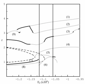
Figure 6: Characteristic curves of nine different families of periodic orbits: (1) -1:1, (2) -1:1 of multiplicity two (bifurcating from the -1:1 family), (3) -2:1, (4) $PL_{1}$, (5) -4:1, (6) 4:1, (7) and (8) 3:1, (9) -1:1. The ordinate yields the radial distance $r$ at one of the apocenters of the respective periodic orbit as a function of the Jacobi constant $E_{J}$. An orbit is stable at black segments and unstable at gray segments of its characteristic curve. The commensurabilities of the periodic orbits refer to the number of radial oscillations per azimuthal period. A minus sign indicates retrograde azimuthal motion. The profiles of the effective potential through $L_{1}$ (inner) and $L_{4}$ (outer) (same as in Fig.3a) are overplotted (dashed curves). The left and right vertical lines at $E_{J}=-1.116\times 10^{6}$ and $E_{J}=-1.06\times 10^{6}$ pass through seven and four unstable families respectively. The manifolds of these families are shown in figures 7a and 10a,b respectively.

3 Unstable periodic orbits and their invariant manifolds

Fig.6 shows the characteristic curves of nine different families of periodic orbits with apocenters close to or beyond the corotation region. The characteristic curves correspond to monoparametric functions $r(E_{J})$, $\theta(E_{J})$ and $p_{\theta}(E_{J})$ yielding the apocentric radius, azimuthal angle and angular momentum for which an orbit with initial conditions $r,\theta,p_{\theta},\dot{r}=0$, and Jacobi constant $E_{J}$ is periodic. Fig.6 shows only the projection $r(E_{J})$ of each characteristic curve. In fact, contrary to the usual plots of characteristic curves (see Contopoulos and Grosbøl 1989 for a review of such curves in barred galaxies), the projection $r(E_{J})$ shown in Fig.6 does not suffice to determine the initial conditions of a periodic orbit, because there is no preferential axis of symmetry in which the apocenters lie. However, these plots are indicative of the radial distances reached by each periodic orbit as a function of the Jacobi constant. The commensurabilities of the periodic orbits correspond to the ratio of the number of radial oscilations (apocentric passages) of an orbit per azimuthal period. Only low order commensurabilities are considered. Finally, the black and gray parts correspond to intervals of value of the Jacobi constant at which the corresponding periodic orbit is stable or unstable respectively.

Some relevant remarks regarding Fig.6 are:

a) For most values of the Jacobi constant beyond $E_{J,L1}$ there are more than one low order periodic orbits which are unstable. The vertical line at $E_{J}=-1.116\times 10^{6}$ shows an example of a value of $E_{J}$ at which the orbits of seven out of the nine considered families are unstable. The invariant manifolds generated by such orbits are studied in detail below.

b) After an initial rise to apocentric values $r_{a}\simeq 1.3r_{corotation}$, the characteristic curve of the $PL_{1}$ family extends almost horizontally to high values of the Jacobi constant. This implies that the apocenters of the $PL_{1}$ family remain always relatively close to the corotation region, and this family plays significant dynamical role for values of $E_{J}$ well above $E_{J,L1}$.

c) For most considered values of $E_{J}$ in Fig.6 we can find at least one unstable periodic with small absolute value of the Hénon stability $|b|$ index. Typically, the dependence of the stability index of one family on $E_{J}$ shows intervals at which there is an abrupt rise of $|b|$ to very high values (of order $10^{3}$ to $10^{4}$), followed by other intervals at which $|b|$ falls to relatively small values. The latter intervals are close to values of $E_{J}$ at which there are transitions from stability to instability (at $|b|=1$). We find numerically that, for almost any value of $E_{J}$ in the considered interval, there is at least one unstable periodic orbit which has a relatively small stability index (below $|b|<3$). This remark is important, because the time of stickiness determined by the invariant manifolds of an unstable periodic orbit depends crucially on the eigenvalue (or stability index) of the orbit. Namely, the stickiness is appreciable only when the stability index is close to unity. Thus, there are periodic orbits at almost any value of the Jacobi constant fulfiling this condition.

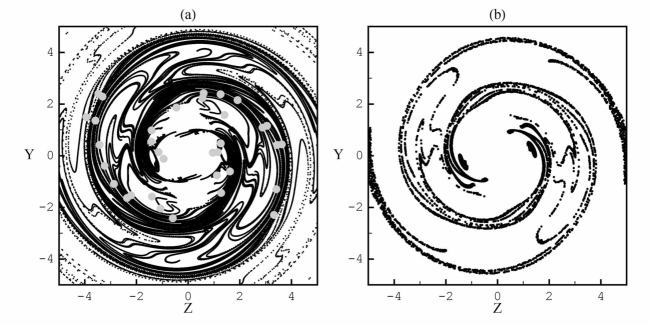
Figure 7: (a) The ‘coalescence’ of invariant manifolds in configuration space for seven different unstable periodic orbits at $E_{J}=-1.116\times 10^{6}$. The orbits are the unstable orbits crossed by the left vertical line of Fig.6, namely (1), (2), (3), (4), (5), (6), and (8). (b) A ‘response model’ with 10000 test particles. The plot shows the third apocentric positions of all these particles, when distributed initially uniformly with respect to the angle $\theta$ along the circular orbit that exists under the monopole term of the potential expansion at the Jacobi constant $E_{J}=-1.116\times 10^{6}$. The gray dots are the same as the dots of figure 1a.

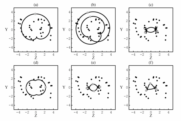
Figure 8: The periodic orbits (a)-1:1, (b) -1:1 of multiplicity 2, (c) -4:1, (d) -2:1, (e) 4:1, and (f) 3:1, at the Jacobi constant $E_{J}=-1.116\times 10^{6}$. The gray dots denote the apocenters of the orbits. The black dots are the same as in figure 1a.

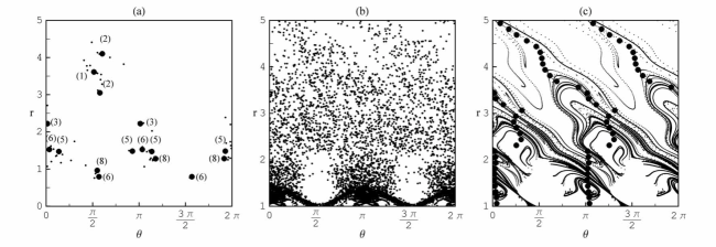
Figure 9: (a) The points of all the N-Body particles within the energy bin $E_{J,L1}\leq E_{J}\leq E_{J,L4}$ which are in the immediate phase space vicinity of the periodic orbits of Fig.8, when the particles’ orbits are brought to their nearest consequent with the surface of section. The particles are located according to the criterion $d_{min,p}\leq 0.04$. The bold circles denote the position of the fixed points of the same periodic orbits on the surface of section. There are 13 nearest particles identified for orbit (1), 6 for orbit (2), 8 for orbit (3), 14 for orbit (5), 13 for orbit (6), and 18 for orbit (8). (b) Successive consequents of the previous particles (up to 100 iterations) on the surface of section. (c) Comparison of the maxima of the density produced by the points of (b) with the coalescence of the invariant manifolds at $E_{J}=-1.116\times 10^{6}$ (the manifolds of PL1 and -4:1 families are plotted).

Figure 7 shows now the main result. The unstable manifolds of seven different families of periodic orbits, which, for $E_{J}=-1.116\times 10^{6}$ are all unstable, are superposed in the same plot of the configuration space (Fig.7a). We immediately recognize that the unstable manifolds of all the families contribute to the formation of the same spiral pattern. In fact, given that the unstable manifold of one periodic orbit cannot intersect the unstable manifolds of other periodic orbits (see, e.g., Contopoulos 2004, pp.144-157), the manifolds emanating from two different periodic orbits describe nearly parallel paths in the configuration space. The so-created set of all the manifolds generates a pattern, that we call the ‘coalescence’ of invariant manifolds. In our case, the shape generated by the coalescence of all the manifolds follows closely that determined by just one manifold, e.g., the manifold of the $PL_{1}$ orbit. We emphasize again that each point in Fig.7a corresponds to an apocentric passage of a chaotic orbit. We thus see that, as many chaotic orbits, with very different initial conditions, describe iterations with apocenters along (or close to) the invariant manifolds of Fig.7a, these orbits are all supporting the same spiral pattern beyond the bar. Comparison with the thick dots of the maxima of the real spiral pattern demonstrates that the real spiral arms are close to the pattern formed by the coalescence of the invariant manifolds (small differences in the two patterns are discussed below).

Patsis (2006) recently reported the results of numerical calculations in a so-called ’response model’ of a barred spiral galaxy, in which, similarly to our example, the spiral pattern is found to be supported mostly by chaotic orbits. A response model is created by taking test particles, placed initially near the circular orbits that exist under the axisymmetric term of the potential. Then, it is found that, after a short integration, the test particles with Jacobi constants close to the value at corotation settle down to positions producing a pattern which has a very good agreement with the observed spiral pattern. In order to understand this behavior, we considered in our model the response of the orbits of 10000 test particles which are initially uniformly distributed within a narrow strip $(\theta,p_{\theta})\in[0,2\pi)\times[p_{\theta,0}-\Delta p_{\theta}/2,p_{\theta,0}+\Delta p_{\theta}/2]$ of the surface of section for $E_{J}=-1.116\times 10^{6}$ (same as in Figure 7a), where $p_{\theta,0}=1.56$ is the angular momentum corresponding to a circular orbit in the monopole potential term at the same value of the Jacobi constant, and $\Delta p_{\theta}=0.03$. Figure 7b shows the projection in the configuration space of the third Poincaré iterates (=iterates of the mapping on the surface of section) of all the 10000 orbits. Clearly, after only three iterates, the orbits of the test particles, which were initially placed along the corotation circle, respond in such a way that the apocenters of all the orbits (Fig.7b) are delineated along a locus which follows essentially the same pattern as that of the invariant manifolds of Fig.7a, i.e., a spiral pattern (figure 7b does not change if the non-axisymmetric part of the potential is introduced gradually). This behavior is understood by noticing that the coalescence of invariant manifolds within a connected chaotic domain creates preferential directions along which the chaotic stretching takes place, so that, after a few transient iterates, the successive images of a set of nearby initial conditions are delineated along these directions (see Voglis et al. (1998) for an example of this behavior in a simple dynamical system). This is precisely what is observed in Fig.7b, which essentially demonstrates that the dynamical response of the orbits beyond the bar is determined by the coalescence of the invariant manifolds.

In order to estimate the relative importance of the various families, other than $PL_{1}$ or $PL_{2}$, in the production of the spiral pattern due to the coalesence of their manifolds, the following calculation was made: the six different periodic orbits were calculated at the Jacobi constant $E=-1.116\times 10^{-6}$ (Figure 8), which is characteristic of the central energy bin $E_{J,L1}\leq E_{J}\leq E_{J,L4}$. Then, the N-body particles of the same bin were identified, which are in the immediate vicinity of each of these periodic orbits. The numerical criterion for such an identification was the following: each periodic orbit can be considered as a smooth curve in phase space, namely it is given by parametric functions $r_{p}(s)$, $\theta_{p}(s)$, $p_{r,p}(s)$, $p_{\theta,p}(s)$, where $s$ is a parameter along the periodic orbit $p$. In numerical calculations we set $s\equiv t^{\prime}$, where $t^{\prime}$ is the time it takes to reach a particular point of the periodic orbit if $t^{\prime}=0$ is the time at a given initial condition of the orbit. Let, now, $(r_{i},\theta_{i},p_{r,i},p_{\theta,i})$ be the position of the i-th N-body particle of the bin at the snapshot of the simulation considered. We then calculate the minimum weighted distance of the body from the periodic orbit given by:

$$d_{min,p}=\min\Bigg{\{}\sqrt{\big{(}{r_{i}-r_{p}(t^{\prime})\over R_{p}}\big{)}^{2}+\big{(}{\theta_{i}-\theta_{p}(t^{\prime})\over 2\pi}\big{)}^{2}+\big{(}{p_{r,i}-p_{r,p}(t^{\prime})\over P_{r,p}}\big{)}^{2}+\big{(}{p_{\theta,i}-p_{\theta,p}(t^{\prime})\over P_{\theta,p}}\big{)}^{2}}~{}:~{}0\leq t^{\prime}\leq T_{period}\Bigg{\}}$$ (5)

were $R_{p}$, $P_{r,p}$ and $P_{\theta,p}$ are weighting factors given by:

$$R_{p}=\int_{0}^{T_{period}}r_{p}(t^{\prime})dt^{\prime},~{}~{}~{}~{}~{}~{}P_{r,p}=\int_{0}^{T_{period}}|p_{r,p}(t^{\prime})|dt^{\prime},~{}~{}~{}~{}~{}~{}P_{\theta,p}=\int_{0}^{T_{period}}p_{\theta,p}(t^{\prime})dt^{\prime}~{}~{}~{}.$$ (6)

A particle is considered to belong to the $\epsilon-$neighborhood of the periodic orbit if $d_{min}<\epsilon$. In the numerical test we set $\epsilon=0.04$ and have collected 72 particles in total in the specific energy bin. This method collects particles near every periodic orbit which are spread all over the orbit. If, however, the particles’ orbits are integrated for a little until they all reach the surface of section, then the particles yield a concentration of points on the surface of section near every fixed point produced by one periodic orbit. These concentrations for the six considered families are shown in Figure 9a. If now the same particles are followed for many time steps, they produce an ensemble of points which all originate from the particular families, i.e., from initial conditions which are far from the $PL_{1}$ or $PL_{2}$ families. This ensemble is shown on the surface of section of Fig.9b, and it clearly produces an $m=2$ pattern with the angles of density maximum depending on $r$ (black points). Superposed to the coalescence of the invariant manifolds (Fig.9c), these points follow a direction which clearly coincides with the preferential directions of the coalescence of invariant manifolds. The numbers of points found around the various orbits (given in the caption of Fig.9) are comparable. This fact indicates that particles which are initially in the vicinity of very different, and distant in phase space, families of periodic orbits, contribute nearly equally to the formation of ‘sticky’ chaotic patterns that follow the coalescence of the invariant manifolds created by all the families.

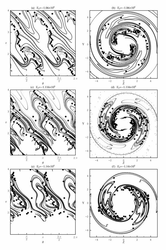
Figure 10: (a,b) Comparison of the loci of the invariant manifolds of the families (1),(2),(4),(5) at the Jacobi constant $E_{J}=-1.06\times 10^{6}$ (right vertical line in Fig.6a), with the maxima of the density of the particles in the energy bin of Fig.3c, obtained via a Fourier decomposition keeping up to the m=4 terms (see text). (c,d) Same for the coalescence of the manifolds at $E_{J}=-1.116\times 10^{6}$ and the particles in the energy bin of Fig.3d (the manifolds of the PL1 and -4:1 families are plotted). (e,f) Same for the manifolds of the family (3) at the Jacobi constant $E_{J}=-1.14\times 10^{6}$ and the particles in the energy bin of Fig.3e.

As the value of the Jacobi constant increases beyond $E_{J,L1}$, we find a progressively smaller number of families playing an important role in the coalescence of invariant manifolds. For example, Figures 10a,b show the superposition of the unstable manifolds emanating from four different periodic orbits which are unstable at the value of the Jacobi constant $E_{J}=-1.06\times 10^{6}$) (right vertical line in Fig.7a). At such a value, which is above both $E_{J,L1}$ and $E_{J,L4}$, the invariant manifolds extend to larger distances away from corotation, but they also penetrate more deeply inside the bar. The black dots correspond to the global maxima with respect to $\theta$, for fixed $r$, of the function:

$$D_{f}(r,\theta)=a_{0}(r)+a_{2}(r)\cos 2\theta+b_{2}(r)\sin 2\theta++a_{4}(r)\cos 4\theta+b_{4}(r)\sin 4\theta$$ (7)

where $a_{2},b_{2},a_{4},b_{4}$ are the coefficients of the Fourier transform, for fixed $r$, of the function

$$D(r,\theta)=\sum_{i=1}^{\mbox{N.of particles}}A\exp\Bigg{(}-{(r_{i}-r)^{2}\over\sigma_{r}^{2}}\Bigg{)}\exp\Bigg{(}-{(\theta_{i}-\theta)^{2}\over\sigma_{\theta}^{2}}\Bigg{)}$$ (8)

which represents a Gaussian-smoothed density obtained by the particles in the same bin of energies as in Fig.3c. The dispersions $\sigma_{r}$ and $\sigma_{\theta}$ are taken equal to the steps $\sigma_{r}=\Delta_{r}$ and $\sigma_{\theta}=\Delta\theta$ of a $50\times 50$ grid in the square $1\leq r\leq 4$ and $0\leq\theta\leq 2\pi$. It is necessary to consider the shift of the maxima induced by the m=4 terms because in some cases such terms reach amplitudes up to about 1/3 of the m=2 term. We see that the maxima of the particles’ density remain are very close to segments of the manifolds, in particular those forming bundles of preferential directions. The maximum phase difference found between the angles of maxima of the particles’ density and the manifolds was 20 degrees, but the typical difference is of a few degrees. Figures 10c,d show the same comparison for the coalescence of the manifolds at $E_{J}=-1.116\times 10^{6}$, and the particles in the associated energy bin (same as in Fig.3d). Finally, Figs.10e,f show the same comparison for the manifolds and particles in the energy bin of Fig.3e, in which the $PL_{1}$ family does not exist. This plot shows that despite the absence of the $PL_{1}$ family, the manifolds of other families continue to support the spiral arms. Furthermore, the energetically allowed outer radial domain is beyond distances $r>1.6$, that is, the manifolds of the particular families support a part of the spiral structure that starts well beyond corotation.

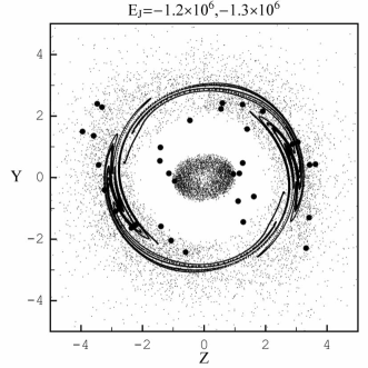
Figure 11: Comparison of the loci of the invariant manifolds of the -1:1 family (curve (9) of Fig.6a) when $E_{J}=-1.222\times 10^{6}$, with the spatial distribution of the N-body particles with Jacobi constants in the interval $-1.2\times 10^{6}>E_{J}\geq-1.3\times 10^{6}$.

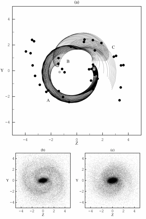
Figure 12: (a) Initial segments of the orbits of 20 initial conditions along the unstable manifold of the $PL_{1}$ family at $E_{J}=-1.116\times 10^{6}$ (b) The projection on the disk plane of the particles with radial velocities satisfying $|v_{r}|<0.1\sqrt{2|E_{J}|}$ at the snapshot $t=47$. (c) Same as (b) for the particles satisfying $|v_{r}|\geq 0.1\sqrt{2|E_{J}|}$.

As the value of $E_{J}$ decreases, the bundles of preferential directions become more and more narrow (Figure 11), and at large distances the patterns generated by the invariant manifolds become more and more axisymmetric. This tendency of the manifolds marks the end of the spiral pattern. The manifold of Figure 11 emanates from a -1:1 unstable periodic orbit. This implies that the end of the spiral pattern in our example is near the outer 1:1 resonance, i.e., beyond the outer Lindblad resonance.

In all the previous figures, the manifolds are plotted on the surface of section corresponding to the apocentric positions of the orbits. On the other hand, the N-body particles are not necessarily close to such positions. A question is, then, why should the apocentric positions be particularly important in the determination of the spiral arms. In paper I, this was explained as a consequence of the fact that the successive apocenters of the chaotic orbits along the manifolds are well correlated in space and time, their correlation being qualitatively described by a soliton type equation. However, a quantitative answer can only be based on numerical evidence, i.e., by considering the behavior in configuration space of orbits with initial conditions on the invariant manifolds, i.e., asymptotic to the periodic orbits. As shown in figure 12a, sufficiently close to $L_{1}$, segments of orbits asymptotic to a $PL_{1}$ periodic orbit support the spiral pattern all along their length, i.e., not only at the apocenters. However, after an azimuthal turn of about $\theta\simeq 3\pi/4$ from $L_{1}$, the asymptotic orbits typically abandon (at point A in figure 12a) the spiral arm emanating from $L_{1}$ and form bridges along which material flows to support either the inner maxima of the $m=2$ pattern( at region B, pericenters), or the other arm of the spiral pattern (region C, apocenters). Orbits having intermediate apocentric passages along the excursion from one to the other arm create the inner spurs of the invariant manifolds observed in the interarm region such as in the invariant manifolds of Figs.7a, or 10.

The importance of the apsidal positions in the support of the overall m=2 pattern can finally by tested simply by plotting separately the N-Body particles being close to the apsides at the given snapshot (figure 12b) from those being far from the apsides (figure 12c). In these figures the separation of the particles is based upon a particle’s radial velocity $|v_{r}|$ being smaller or greated than $0.1\sqrt{2|E_{J}|}$, where $E_{J}$ is the particle’s Jacobi constant. Figs.12b,c show that the particles being near their apsides form a distribution that clearly describes the spiral maxima, while the particles far from the apsides contribute rather marginally to the spiral pattern.

All these effects notwithstanding, it should be stated clearly that the theory developed so far only suggests that the phenomenon of the coalescence of the invariant manifolds of the unstable periodic orbits near or beyond corotation constitutes a key concept in order to understand the dynamics of the spiral arms in barred galaxies. Other phenomena mentioned in section 2, as, for example, the secular evolution of the bars, or the presence of more than one pattern speeds, cannot be covered by the presently exposed theory. Thus, a subject of further study regards incorporating the concept of the coalescence of the invariant manifolds into a more complete theory for the role of chaos in the dynamics of the spiral arms in barred galaxies.

4 Conclusions

In this paper, which is a continuation of our previous work (paper I, Voglis et al. 2006), we examine the role played by the invariant manifolds of many different families of unstable periodic orbits near and beyond corotation in supporting a spiral pattern beyond the bar of a rotating barred - spiral galaxy. Our study was based on an N-Body model of such a galaxy. The main conclusions are the following:

1) One of the main topological properties of the invariant manifolds of unstable periodic orbits co-existing at the same value of the energy (Jacobi constant) is that the unstable (stable) manifolds of one family cannot intersect the unstable (stable) manifolds of any other family. As a result, the unstable manifolds of all the families are forced to follow nearly parallel paths in either the phase space or the configuration space. We call the overall pattern produced by the superposition of the invariant manifolds of all the different families a ‘coalescence’ of invariant manifolds.

2) The coalescence of invariant manifolds produces a locus in configuration space yielding a spiral pattern. Every point on this locus is a local apocentric position of a chaotic orbit. This locus is invariant under a Poincaré mapping of the orbital flow. That is, as the particles on chaotic orbits are mapped by the orbital flow from one apocentric passage to the next apocentric passage, the successive apocenters reached by the particles are all on the same locus determined by the coalescence of invariant manifolds.

3) The real observed spiral pattern of the system coincides with the spiral pattern produced by the coalescence of invariant manifolds. We explain this as a stickiness phenomenon. Namely, while the phase space is open and the chaotic orbits in general escape within only a few radial periods to distances far from corotation, the chaotic orbits with initial conditions close to the invariant manifolds remain trapped to ‘sticky’ orbits near the manifolds for times of order 100 dynamical periods.

4) Different families of unstable periodic orbits play the dominant dynamical role in the above phenomena at different values of the Jacobi constant. The short period unstable family $PL_{1}$, which in our previous work (paper I) and in the work of others (Romero-Gomez et al. 2007) was identified as the main family responsible for the spiral pattern, is found to play an important role for values of the Jacobi constant $E_{J}>E_{J,L1}$, which is however amplified by the extentions of other families near corotation, e.g., the 3:1 and 4:1 families.

5) The main contribution to the spiral pattern is by the manifolds of families which are unstable in the energy range $E_{J,L1}\leq E_{J}\leq E_{J,L4}$. These manifolds support both the edge of the bar and the spiral structure close to and outside corotation.

6) The manifolds of families which are unstable for $E_{J}<E_{J,L1}$ are responsible for extensions of the spiral arms at distances well beyond corotation. Beyond the outer Lindblad resonance, the patterns formed by the invariant manifolds become more and more axisymmetric, and this tendency marks the end of the spiral arms.

Acknowledgements: P. Tsoutsis was supported in part by a research grant of the Research Committee of the Academy of Athens. We thank Prof. G. Contopoulos for many suggestions and a careful reading of the manuscript, as well as an anonymous referee for the numerous comments that improved the paper considerably. This work started in collaboration with our teacher and beloved friend N. Voglis, who passed away on February 9, 2007.

References

- (1) Aguerri, J.A.L., Beckman, J.E., and Prieto, M.: 1998,Astron. J. 116, 2136.
- (2) Allen, A.J., Palmer, P.L., and Papaloizou, J.: 1990, Mon. Not. R. Astr. Soc. 242, 576.
- (3) Contopoulos, G.: 1985, Comments on Astrophysics 11, 1.
- (4) Contopoulos, G. and Grosbøl, P.: 1986, Astron. Astrophys. 155, 11.
- (5) Contopoulos, G. and Grosbøl, P.: 1988, Astron. Astrophys. 197, 83.
- (6) Contopoulos, G. and Grosbøl, P.: 1989, Astron. Astrophys. Rev. 1, 261.
- (7) Contopoulos, G., Harsoula, M., : 2008, Int. J. Bif. Chaos (in press).
- (8) Contopoulos, G.: 2004, “Order and Chaos in Dynamical Astronomy”, Springer-Verlag.
- (9) Efthymiopoulos, C., and Voglis, N: 2001, Astron. Astrophys. 378, 679.
- (10) Efthymiopoulos, C., Contopoulos, G., Voglis, N., and Dvorak, R.: 1997, J. Phys. A 30, 8167.
- (11) Hernquist, L.: 1987, Astrophys. J. Suppl. 64, 715.
- (12) Gadotti, D.A., and de Souza, R.E.: 2006, Astrophys. J. Suppl. 163 270.
- (13) Grosbøl, P.: 1994, in G. Contopoulos, N. Spyrou and L. Vlahos (Eds), “Galactic Dynamics and N-Body Simulations”, Lecture Notes in Physics, 433, 101.
- (14) Kaufmann, D.E. and Contopoulos, G.: 1996, Astron. Astrophys. 309, 381.
- (15) Lindblad, P.A.B., Lindblad, P.O., and Athanassoula, E: 1996, Astron. Astrophys. 313, 65.
- (16) Michel-Dansac, L., and Wozniak, H.: 2006,Astron. Astrophys. 452, 97.
- (17) Palmer, P.L., and Voglis, N.: 1983, Mon. Not. R. Astr. Soc. 205, 543.
- (18) Patsis, P.A., Contopoulos, G. and Grosbøl, P.: 1991, Astron. Astrophys. 243, 373.
- (19) Patsis, P.A., Hiotelis, N., Contopoulos, G. and Grosbøl, P.: 1994, Astron. Astrophys. 286, 46.
- (20) Patsis, P.A. and Kaufmann, D.E.: 1999, Astron. Astrophys. 352, 469.
- (21) Romero-Gomez, M., Masdemont, J.J., Athanassoula, E. and Garcia Gomez, C.: 2006, Astron. Astrophys. 453, 39.
- (22) Romero-Gomez, Athanassoula, E.M., Masdemont, J.J., and Garcia-Gomez, C.: 2007, Astron. Astrophys. 472, 63.
- (23) Sparke, L.S. and Sellwood, J.A.: 1987, Mon. Not. R. Astr. Soc. 225, 653.
- (24) Voglis, N., Contopoulos, G., and Efthymiopoulos, C, 1998, Phys. Rev. E, 57, 372.
- (25) Voglis, N., Tsoutsis, P., and Efthymiopoulos, C., 2006a, Mon. Not. R. Astr. Soc. 373, 280.
- (26) Voglis, N., Stavropoulos, I., and Kalapotharakos, C., 2006b, Mon. Not. R. Astr. Soc. 372, 901.
- (27) Zel’dovich, Ya: 1970, Astron. Astrophys. 5, 89.